Can Lumped Characteristics of a Contributing Area Provide Risk Definition of Sediment Flux?

Abstract

Accelerated soil erosion by water has many offsite impacts on the municipal infrastructure. This paper discusses how to easily detect potential risk points around municipalities by simple spatial analysis using GIS. In the Czech Republic, the WaTEM/SEDEM model is verified and used in large scale studies to assess sediment transports. Instead of computing actual sediment transports in river systems, WaTEM/SEDEM has been innovatively used in high spatial detail to define indices of sediment flux from small contributing areas. Such an approach has allowed for the modeling of sediment fluxes in contributing areas with above 127,484 risk points, covering the entire Czech Republic territory. Risk points are defined as outlets of contributing areas larger than 1 ha, wherein the surface runoff goes into residential areas or vulnerable bodies of water. Sediment flux indices were calibrated by conducting terrain surveys in 4 large watersheds and splitting the risk points into 5 groups defined by the intensity of sediment transport threat. The best sediment flux index resulted from the correlation between the modeled total sediment input in a 100 m buffer zone of the risk point and the field survey data (R² from 0.57 to 0.91 for the calibration watersheds). Correlation analysis and principal component analysis (PCA) of the modeled indices and their relation to 11 lumped characteristics of the contributing areas were computed (average K-factor; average R-factor; average slope; area of arable land; area of forest; area of grassland; total watershed area; average planar curvature; average profile curvature; specific width; stream power index). The comparison showed that for risk definition the most important is a combination of morphometric characteristics (specific width and stream power index), followed by watershed area, proportion of grassland, soil erodibility, and rain erosivity (described by PC2).

1. Introduction

Rainfall-runoff events leading to soil erosion can also cause extensive off-site effects, damage to the urban infrastructure, and can endanger human lives [1,2].

Various models can be used for modeling erosion and sediment transport. In general, these models can be categorized as empirical/statistical, conceptual, and process-based [3]. The models differ in the number of required inputs. Moreover, the quality and the representativeness of the model outputs is very variable. Empirical models based on the universal soil loss equation [1,4,5,6] are widely used for determining the erosion threat over large areas. In the Czech Republic, the RUSLE-based WaTEM/SEDEM model [7,8,9] is verified and used in large scale studies [10,11,12,13]. This model provides a sufficiently accurate estimate of the erosion intensity and the amount of transported soil material on the basis of a relatively small amount of input data [14].

The spatial resolution and quality of input data for RUSLE-based models in the Czech Republic is rather high, and the method is also used for cross compliance policy application here [15]. Therefore, WaTEM/SEDEM outputs were considered as a relevant basis for definition of sediment flux risk in residential areas for the entire Czech Republic in the framework of research project VG20122015092: “Erosion Runoff—Increased Risk of the Residents and the Water Quality Exposure in the Context of the Expected Climate Change”.

Instead of computing actual sediment transports in river systems, WaTEM/SEDEM was innovatively used in high spatial detail, but only to define indices of sediment flux from small contributing areas. Such an approach allowed for the modeling of sediment fluxes in contributing areas with above 127,484 risk points, covering the entire Czech Republic territory (78,866 km²). Risk points are defined as outlets of contributing areas larger than 1 ha [16], wherein the surface runoff goes into residential areas or vulnerable bodies of water (presented in detail in Section 2.1). Sediment flux indices are calibrated by conducting terrain surveys and splitting the risk points into 5 groups defined by the category of the sediment transport threat (1 to 5). In the following text, the contributing areas of the risk points are called “risk watersheds”.

Erosion-related lumped watershed characteristics [17] can be divided into several groups: Morphological, morphometric, land use (presence and state of vegetation), soil quality characteristics, and climatic (precipitation characteristics). The most commonly observed parameter is the slope, which seems to be crucial for the transition from soil cover disturbance to transportation of eroded particles down the slope [18]. The parcel or watershed slope is an important factor for the effectiveness of erosion control measures [19], but this is related to land use [20]. The morphometric parameters, especially the shape of the watershed and the predominant shape of the slopes (convergent/divergent, convex/concave) are important for a description of the rainfall-runoff, erosion, and transport process. The impact of the shape of a watershed, expressed by the specific width (watershed area/watershed length), the planar curvature (describing the convergence/divergence of the slopes), the curvature of the profile (describing the convexity/concavity of the slopes), indices expressing the hydrological behavior, and the erodibility of the watershed and the other morphometric parameters, has been described and assessed in a number of studies [16,21,22,23]. All watershed characteristics interact, and together they determine the final level of the threat of intensive sediment flux.

Another novelty of this paper lies in correlation analysis and principal component analysis (PCA) of the modeled data and their relation to general watershed (contributing area) characteristics. This way, the sensitivity of model outputs to the general watershed parameters could also be tested. The motivation was the awareness that in many large regions the data of the same spatial resolution and quality (as in the Czech Republic) are not available [24,25]. The research questions are therefore:

• What are typical parameters of a Czech watershed that produces a considerable amount of eroded material and should be modeled in more detail by a process-based model?
• Can single lumped contribution area parameters replace WaTEM/SEDEM modeling if we want to define five classes of the threat of sediment flux (e.g., not having a detailed DEM (Digital elevation model) or spatially detailed land-use maps or soil maps)?
• Can a statistically selected combination of these characteristics provide a better estimate?

If the lumped source area characteristics can define the overall sediment flux risk, the approach can then be used for simplifying the sediment transport assessment methods for regions with a lack of WaTEM/SEDEM input data in a relevant level of detail.

The aim of the study is to use an extensive set of results of the VG20122015092 project to derive a simplified statistical approach. Based on the characteristics of the watershed, which can be easily identified on the basis of open source data, it would then be possible to identify localities where the threat of intensive sediment runoff is high. Measures into the most high-risk areas can be then designed by process-based models.

2. Materials and Methods

2.1. Definition of Source Areas and Risk Points

First, raster-based GIS input data in 10 m spatial resolution were prepared for the entire area of the Czech Republic, consisting of following layers:

• Digital elevation model (DTM) based on 1:10,000 scale vector contours enhanced by a stereophotogrammetrical model in newly developed areas. Model was corrected for artificial sinks in arable areas;
• Land use, defined by the Fundamental Base of Geographic Data of the Czech Republic (http://geoportal.cuzk.cz/(S(aypz0pbaffy4rwohh4fljcu2))/default.aspx?lng=EN&mode=TextMeta&text=dSady_zabaged&side=zabaged&menu=24), and updated by the national register of agricultural areas (Land Parcel Identification System, 1:10,000 scale).

Second, flow accumulation over the entire Czech territory was provided, respecting fragmentation of the DTM by land use (roads, other linear structures, and built-up areas).

Contributing areas larger than 1 ha [26] had defined drainage networks potentially at risk of resulting in concentrated overland flows and sediment transport. By intersecting the drainage network with the boundaries of residential areas, the risk points were defined. Residential areas were identified as “all built-up classes” including gardens up to 50 m from house polygons. Rural gardens (parks) were excluded.

All risk points were considered as potential outlets of sediment flux, so for every point a source area was delineated (called “watershed” in further text). To reduce the number and spatial frequency of the points in the presented results for municipality communities, the risk points closer than 50 m and their watersheds were grouped assuming these outlets are always entering into the same part of any residential area.

The analysis resulted in 127,484 risk points and their watersheds. Further analyses were focused on the definition of the threat (in five classes) to define which points have no risk of sediment flux and which can lead to infrastructure damages. WaTEM/SEDEM was used to define the levels of threat of intensive sediment flux entering residential zones from these watersheds. After extensive terrain surveys and comparison with the model results, the modeled sediment inflow into 100 m buffer zones around residential areas was used as the proper parameter for risk definition.

2.2. Sediment Transport Modeling

For sediment transport modeling and for definitions of indices of erosion threat in risk points, the WaTEM/SEDEM model was used [7,8,9]. WaTEM/SEDEM is a RUSLE-based model (Equation (1)):

$$A=R\times K\times C\times LS\times P$$

(1)

where: A—annual soil erosion rate (Mg/ha·year), R—rainfall erosivity factor (MJ·cm/ha·h·year), K—soil erodibility factor (Mg·h/MJ·cm), LS—topographic factor (-), C—crop management factor (-), and P—erosion control practice factor (-).

Unlike RUSLE, WaTEM/SEDEM calculates the sediment transport capacity based on Equation (2) in each pixel, and then balancing every pixel, it determines the erosion/deposition:

$$TC=K_{TC}\times E{p}_{rill}$$

(2)

where: TC—transport capacity (Mg/ha·m), K_TC—transport capacity coefficient (m), and Ep_rill—potential for rill erosion (Mg/ha·year).

A detailed description of the model structure and its parametrization for the Czech Republic is provided by [27].

Distributed R-factor values in 1-km resolution were derived by Hanel [28,29]. Typical C-factor values for land use categories in the Czech Republic are defined by Janeček [30] in accordance with the USDA handbook 537 [4]. The C-factor for arable land was determined as an average value according to the logged crop rotation [31] in each territorial unit (76 districts). A DEM with a spatial resolution of 10 m was used for calculating the LS-factor. K-factor values were determined in accordance with the national methodology [32] based on soil quality maps (BPEJ, 1:5000 scale).

In the Czech Republic and in the 10-m resolution data used in this study, WaTEM/SEDEM was calibrated previously in the Rimov watershed (488 km²) by [27]. Based on the calibration, the following internal parameters of WaTEM/SEDEM were used in this study: PTEF (arable, forest, grassland = 0, 75, 75); parcel connectivity (arable, others = 40, 75); KTC (arable, others = 35, 55).

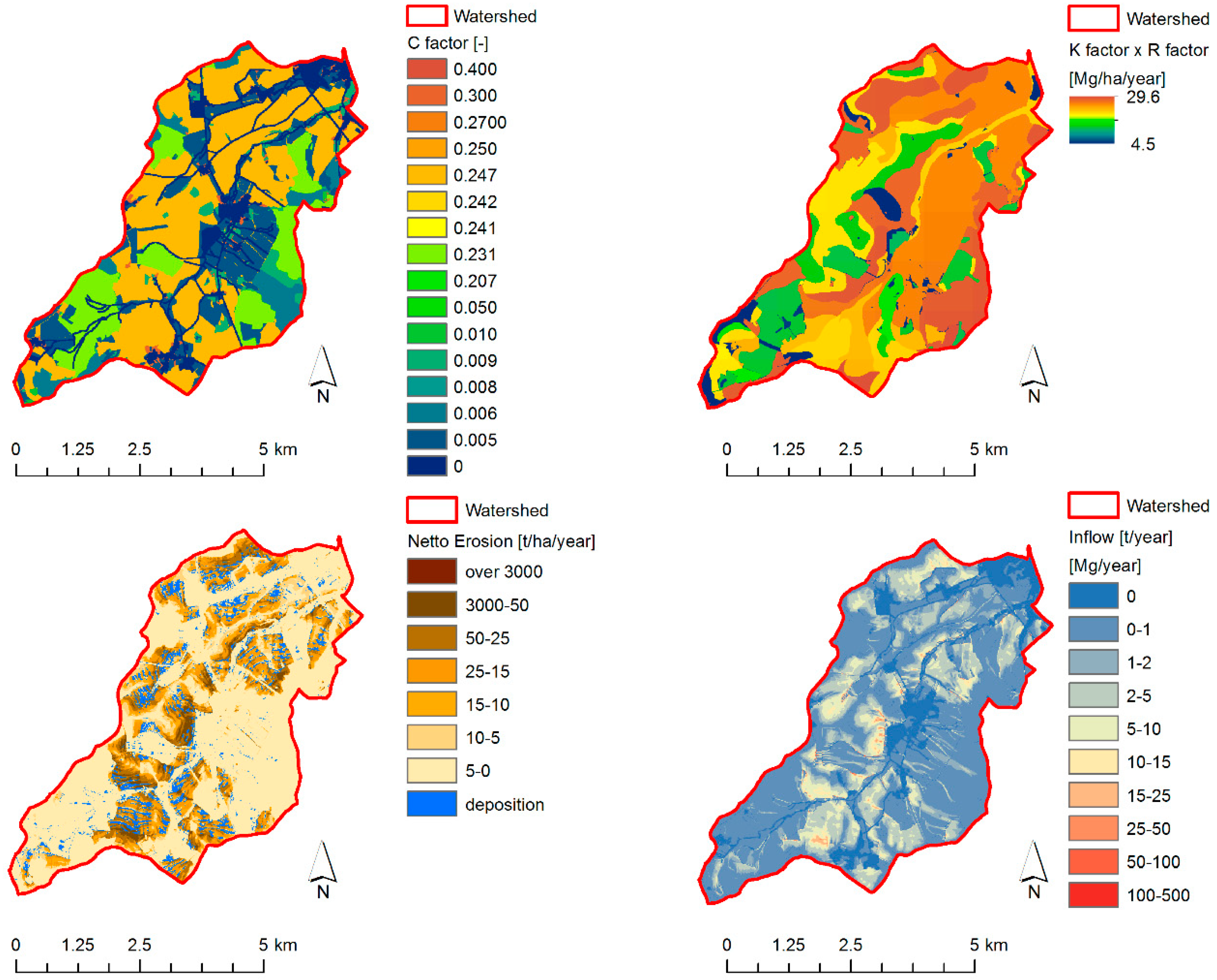
Modeling (in tiles) was provided over the entire area of the Czech Republic, considering all surface waters and residential areas as points of delivery (in the terminology of WaTEM/SEDEM, the “river” class of land use). The fully distributed modeling of sediment transports within streams applying river topology maps and reservoirs was out of the scope of the project. Therefore, the model was only used to derive an erosion/deposition map (called “netto erosion”) and sediment transport map (called “inflow”). Model output, together with selected model input data, are in Figure 1.

Raster-based GIS outputs (netto erosion and inflow) were further analyzed by zonal statistics of all 130,000 watersheds to provide risk classification concerning sediment fluxes. Here we should point out that the original calibration could also be used because the actual values of sediment transports in outlet points were not of importance. The only need was to define the high-risk and low-risk classes of the sediment entrance into residential areas, and not to compute the transported sediment volumes.

2.3. Evaluation of the Level of Threat

The level of the threat of sediment transport into residential areas was determined for the risk points. The aim was to classify the risk points into five classes depending on potential sediment fluxes. Since the contributing areas of the risk points were starting only with 1 ha size, for many watersheds we could assume rather high sediment connectivity [33]. Therefore, not only WaTEM/SEDEM sediment delivery to the outlet (inflow) was considered, but also total soil loss and area-specific soil loss in each watershed (example of watershed in Figure 2).

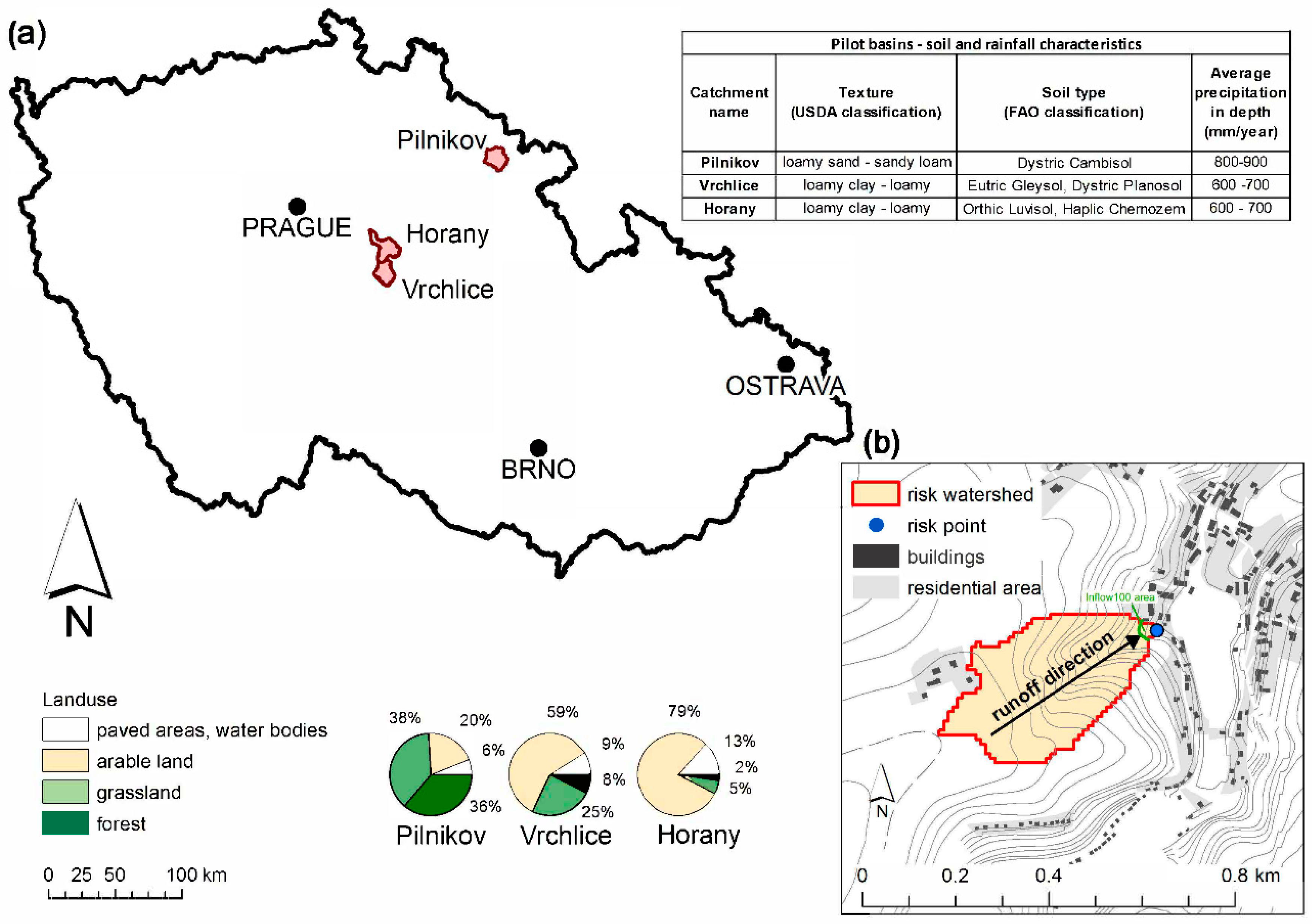
Optimal approach for classifying all risk points would be the terrain survey, but the 79,000 km² and 130,000 risk points could not be visited. For that reason, three research catchments (of ca. 100 km² each) were selected (Figure 2) to correctly set the five threat categories by terrain survey. The basins represent the most common types of agricultural landscape in the Czech Republic. The Horany Basin represents intensively used lowlands with large parcels, long straight slopes, and intensive crops (corn, sugar beet, and cereals). The Vrchlice Basin represents upland landscapes with morphologically diverse watersheds, steeper slopes, and intensive agriculture, and the Pilnikov Basin represents foothills with steep convergent slopes, and a high proportion of cereals, forage, and grassland. In these basins, the real threat categories (1–5) for the risk points were identified by field surveys. The field survey results were compared with the zonal statistics of the WaTEM/SEDEM outputs for each risk watershed to select a suitable model result for defining the threat categories.

The entire area of the watershed, soil erosion potential and evidence, the runoff trajectory, and the watershed outlets into residential areas were observed. Concurrently, the real sediment transport pathways in pre-selected profiles were surveyed. Information from residents about previous intensive sediment flux was an important aspect of the field survey.

WaTEM/SEDEM modeling provided the output GIS layers for the soil loss, the sediment transport/deposition in each pixel (netto erosion), and the total sediment input in each pixel (inflow). First, it was necessary to choose a best fitting model output for the correct description of the real threat defined by five classes based on the terrain survey.

The tested model outputs of the model were (

Table 1. Correlation (correlation coefficient) between tested model outputs value and threat category determined within field survey.

	Aspecific	Atotal	Inflow100
Horany	0.27	0.46	0.57
Pilnikov	0.16	0.63	0.76
Vrchlice	0.34	0.56	0.91
Complete field survey	0.23	0.46	0.70

A_specific—the specific soil loss in the watershed, A_total—the total soil loss in the watershed, Inflow100—sediment transport, the total sediment input in a 100-m buffer zone of the potentially threatened outlet.

):

• Aspecific (Mg/ha·year)—the specific soil loss in the watershed;
• Atotal (Mg/pixel·year)—the total soil loss in the watershed;
• Inflow100 (Mg/year)—sediment transport to the outlet, the total sediment input in a 100-m buffer zone of the risk point.

The statistical values of the tested model outputs were calculated for threat watersheds in the calibration areas. Then the relationship between the model outputs values and the threat category was evaluated. The Inflow100 was shown to be the most suitable model output for the threat of sediment delivery into the risk point (Table 1).

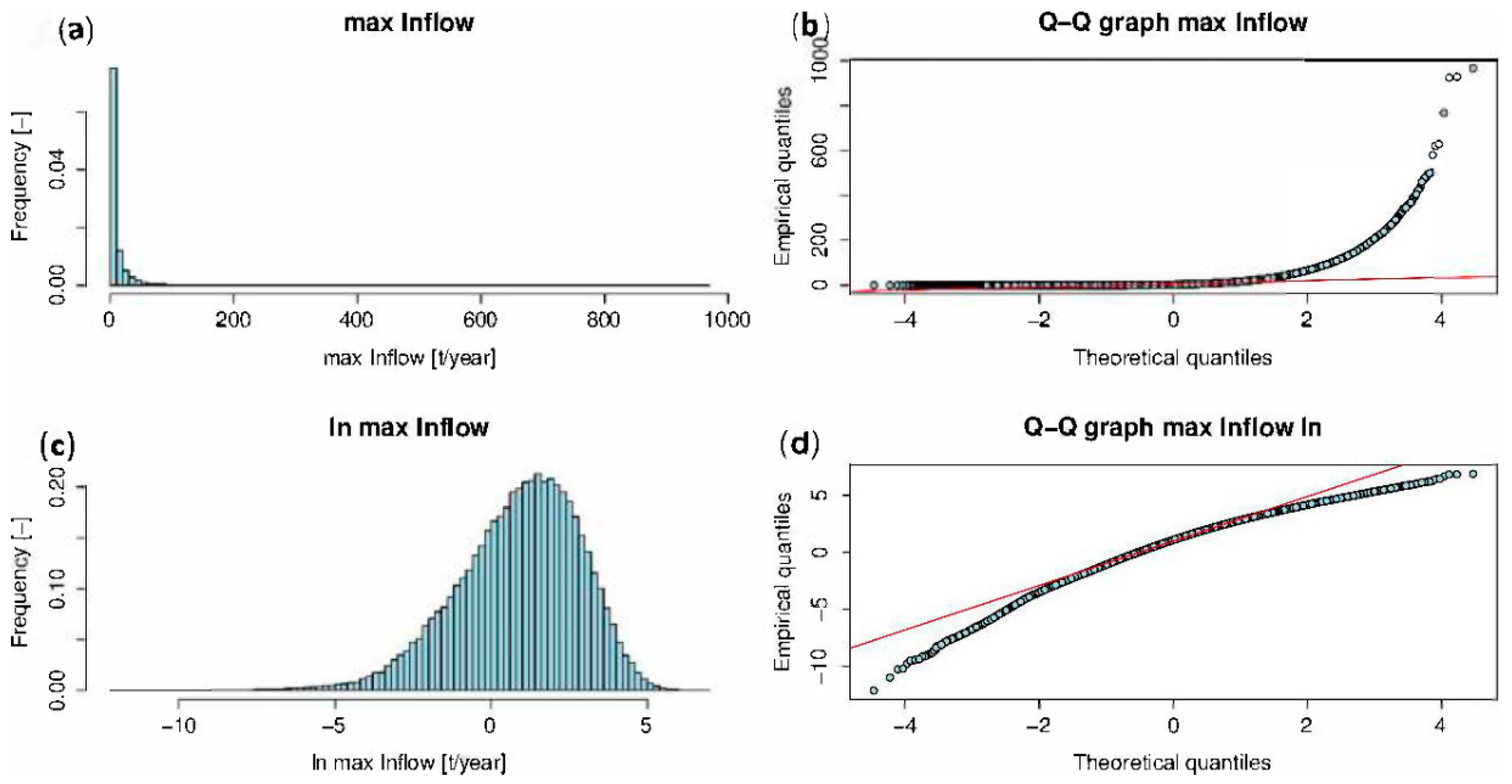
In the complete database of threat watersheds for the Czech Republic, the Inflow100 ranges from 0 to 966 Mg/year. The distribution of values shows that the frequency of lower Inflow100 values is higher than the frequency of higher Inflow100 values. The statistical distribution of Inflow100 values in the watershed database was determined in order to set the threshold for the Inflow100 values that define the five threat level categories. Normal distribution was excluded on the basis of the histogram and the Q-Q plot (Figure 3a,b). The statistical distribution of the Inflow100 values corresponds to the log-normal statistical distribution [34] (Figure 3c,d). The expected distribution of the watersheds (in the complete database) in the sediment transport categories indicates that the threat level is not evenly distributed. Watersheds in threat category 4 or 5 appear less frequently than watersheds in category 1 (very low threat level).

2.4. Impact of Watershed Characteristics on the Threat

The following watershed characteristics are assessed for their impacts on the level of threat of sediment flux in comparison with the results of WaTEM/SEDEM modeling.

Soil characteristics (soil texture, soil structure, amount of organic material) are expressed in the K-factor. The precipitation characteristics (average number of intensive rainfall events during the year and their erosivity) are expressed in the R-factor. The average K-factor and R-factor were assessed for each watershed to simulate low-resolution data comparison. The land use was described by the proportion of arable land, forest, and grassland. The morphological characteristics were included in the analysis through the average slope (%) and the watershed area (ha). The analyzed morphometric characteristics were the specific width of the watershed (m), i.e., the ratio between the area of the watershed and the longest runoff line, the curvature of the profile (in the maximum slope direction)—Curveprofile, and the planar curvature (perpendicular to the direction of the maximum slope—Curveplane [35]. The hydrological index stream power index (m rad) (SPI) was considered.

SPI expresses the erosion potential of the surface runoff. It reflects the drainage area and the slope in a specific location in the watershed, on the basis of Equation (3) [36]:

$$SPI=A_s·s$$

(3)

where SPI is the local stream power index (m rad), A_s is the local specific drainage area per unit contour length, and s is the local slope (%).

First, the correlation matrix expressing the relationship between the Inflow100 and the analyzed watershed characteristics was set up. Based on our analysis of almost 130,000 potentially threatened points, it can be assumed that there is a higher threat level in watershed with a high proportion of arable land, a steep average slope and a specific width, a large watershed area, and a high value of the SPI coefficient. A multi-variate statistical technique was run to verify this assumption. Within this analysis, we tested the relationships among the watershed characteristics that are important for the Inflow100 (or for the final threat category). Principal component analysis (PCA) is one of the most widely used types of multi-variate data analysis [37]. This method simplifies the complexity in high-dimensional data while retaining trends and patterns. It does this by transforming the data into fewer components, which describe a combination of observed dimensions [38]. In the presented analyses, the PCA method transfers the variables (the threat watershed characteristics) to the principal components. The principal components are a linear combination of the original variables (watershed characteristics). The main aim of this transfer is to reduce the number of variables. R studio software [39] was used for the statistical analyses.

3. Results

The Inflow100 values for the thresholds were set (

Table 2. Number of threat watersheds in five threat categories.

	Category 1	Category 2	Category 3	Category 4	Category 5	Total
Range (Inflow100 value)	0–2	2–7	7–20	20–55	>55
Watersheds in category	53,835	32,596	24,389	12,780	3884	127,484

) on the basis of the log-normal distribution of the Inflow100 values and required logarithmic representation of the watersheds in the threat categories. The final number of watersheds in the threat categories corresponds to the logarithmic function.

Table 3. Average values of the analyzed characteristics in risk watersheds representing the five threat categories.

Watershed Characteristics			Category 1	Category 2	Category 3	Category 4	Category 5
Average K-factor	(Mg h/MJ cm)	mean	0.36	0.38	0.39	0.40	0.41
		range	0.60	0.57	0.46	0.53	0.44
		1st and 3rd quartile distance	0.15	0.15	0.14	0.14	0.13
Average R-factor	(MJ cm/ha h year)	mean	63	64	65	67	69
		range	111	111	113	110	112
		1st and 3rd quartile distance	21	19	17	16	15
Average Slope	(%)	mean	9	11	12	13	15
		range	113	83	63	65	72
		1st and 3rd quartile distance	10	11	10	9	9
Area of Arable Land	(%)	mean	35	52	59	62	63
		range	100	100	100	100	100
		1st and 3rd quartile distance	86	96	83	68	61
Area of Forest	(%)	mean	30	28	25	25	27
		range	100	100	100	100	100
		1st and 3rd quartile distance	61	55	43	41	42
Area of Grassland	(%)	mean	35	20	17	14	11
		range	100	100	100	98	98
		1st and 3rd quartile distance	73	33	25	20	15
Total Watershed Area	(ha)	mean	7.12	9.7	14.24	19.77	30.81
		range	1524.96	2238.15	1619.27	1374.07	813.49
		1st and 3rd quartile distance	3.51	6.56	11.50	18.23	30.65
Average Planar Curvature	(-)	mean	0.00	0.00	−0.01	−0.01	−0.02
		range	1.50	1.29	0.96	1.28	0.51
		1st and 3rd quartile distance	0.03	0.03	0.03	0.03	0.03
Average Profile Curvature	(-)	mean	0.00	−0.01	−0.01	−0.01	−0.02
		range	4.21	1.57	1.55	0.89	0.53
		1st and 3rd quartile distance	0.03	0.03	0.03	0.03	0.03
Specific Width	(m)	mean	15	16	16	17	17
		range	419	116	53	88	34
		1st and 3rd quartile distance	5	5	5	5	4
Stream Power Index	(m rad)	mean	1257	2057	2697	3728	5571
		range	488,700	174,800	59,510	105,000	50,820
		1st and 3rd quartile distance	1376.1	2267.6	2785.3	3600	4881

shows the average values for the analyzed characteristics in groups of risk watersheds forming the five threat categories.

An analysis was made of the simple linear correlation between Inflow100 values and individual analyzed characteristics. The correlation matrix (

Table 4. Correlation matrix between Inflow100 and studied characteristics.

	Max Inflow100	Average K-Factor	Average R-Factor	Average Slope	Area of Arable Land	Area of Forest	Area of Grassland	Total Watershed Area	Average Curveplane	Average Curveprofile	Specific Width	Stream Power Index
	(Mg/year)	(Mg h/MJ cm)	(MJ cm/ha h year)	(%)	(%)	(%)	(%)	(ha)	(-)	(-)	(m)	(m rad)
Max Inflow100	1.00
Average K-factor	0.11	1.00
Average R-factor	0.08	0.03	1.00
Average Slope	0.13	0.08	0.24	1.00
Area of Arable Land	0.13	0.02	−0.23	−0.57	1.00
Area of Forest	−0.02	0.28	0.11	0.57	−0.67	1.00
Area of Grassland	−0.15	−0.33	0.17	0.09	−0.55	−0.24	1.00
Total Watershed Area	0.17	0.05	−0.06	−0.03	0.04	0.03	−0.08	1.00
Average Curveplane	−0.10	−0.01	0.07	0.01	−0.03	0.01	0.02	−0.01	1.00
Average Curveprofile	−0.06	−0.03	0.02	−0.11	0.02	−0.09	0.06	0.03	0.39	1.00
Specific Width	0.12	−0.03	−0.08	−0.21	0.11	−0.09	−0.05	0.30	−0.09	0.00	1.00
Stream Power Index	0.30	0.09	0.11	0.49	−0.29	0.34	−0.02	0.32	−0.08	−0.09	0.38	1.00

) shows a considerable relationship (R > 0.20) only between the Inflow100 and stream power index (SPI). The value of the correlation coefficient between Inflow100 and SPI is 0.30.

Table 3 documents the relationship between the threat category of intensive erosion runoff formation and the average values of the selected characteristics. The SPI coefficient and the proportion of arable land, total area, slope, and specific width increases with higher threat categories. The proportion of grassland decreases and the proportion of forest slightly decreases.

The PCA results for the complete database in

Table 5. The variability proportion explained by components (PC1–PC11).

	PC1	PC2	PC3	PC4	PC5	PC6	PC7	PC8	PC9	PC10	PC11
Proportion Explained	0.24	0.16	0.14	0.12	0.08	0.07	0.06	0.05	0.05	0.02	0
Cumulative Proportion	0.24	0.4	0.54	0.66	0.75	0.81	0.87	0.93	0.98	1	1

show the interdependence of the characteristics and the complexity of the relationship between the characteristics and the Inflow100. The individual components explain only a relatively low proportion of the data.

The correlation coefficients between the studied characteristics and five components are presented in

Table 6. Correlation coefficients between the characteristics and components PC1–PC5.

		PC1	PC2	PC3	PC4	PC5
K	(Mg h/MJ cm)	0.17	0.42	−0.53	0.21	0.22
R	(MJ cm/ha h year)	0.36	−0.26	0.06	0.07	0.87
Slope	(%)	0.84	−0.04	−0.11	−0.01	−0.04
Arable land	(%)	−0.8	0.34	−0.16	0.04	0.2
Forest	(%)	0.8	0.19	−0.34	0.12	−0.21
Grassland	(%)	0.2	−0.65	0.58	−0.19	−0.03
Area	(ha)	0.06	0.54	0.44	0.24	−0.02
Curveplane	(-)	−0	−0.3	−0.02	0.78	−0.06
Curveprofile	(-)	−0.1	−0.26	0.13	0.77	−0.08
Spec. width	(m)	−0.1	0.56	0.6	0.07	0.07
SPI	(m rad)	0.6	0.5	0.37	0.06	0.04

. The correlation coefficients between the Inflow100 and the components (PC1–PC5) were calculated to identify the importance of the components (and indirectly of the characteristics) in relation to the level of threat (

Table 7. Correlation coefficients between components (PC1–PC5) and Inflow100.

R between PC and Inflow100
PC1	0.07
PC2	0.28
PC3	0.05
PC4	0.00
PC5	0.17

).

PC2 (R = 0.28) and PC5 (R = 0.17) are relatively important. PC2 has positive relationship with the watershed area, the specific width, the SPI, and the K-factor. Conversely, the proportion of grassland has a negative relationship with PC2. PC5 correlates considerably only with the R-factor.

4. Discussion

The accuracy of the modeled Inflow100 value is importantly influenced by the description of watershed connectivity. The index of connectivity based on GIS analysis of landscape was derived by Borselli [33]. Consequently, it was refined by Cavalli [40]. An essential input for determining watershed connectivity is a digital terrain model with high resolution. Therefore, the connectivity based on high-resolution DEM was not evaluated. The connectivity is involved in modeling by respecting parcel boundaries and by setting a sediment transport capacity within WaTEM/SEDEM. Based on our testing [41] and calibrating of the model in numerous previous studies [10,11,12,13] we believe in reliable results in defining risk of the sediment fluxes from watersheds of average size of 11.3 ha.

A combination of principal component analysis and correlation analysis between the component values and the Inflow100 shows that the most important watershed characteristics for the threat of sediment flux are morphometric characteristics (the shape of the watershed, expressed by the specific width and SPI), the watershed area, the soil erodibility, and the proportion of grassland. The studies focused on the important factors affecting the value of sediment transport show that the influence of these factors depends on the size of the evaluated watershed. Morphological and morphometric factors are particularly significant for smaller watersheds. The area is a key factor influencing sediment transport in larger watersheds [42]. The presence and state of vegetation cover is also important for runoff generation, erosion intensity, and nutrient transport. [1,43]. The soil quality (organic material content, soil structure and texture) influences infiltration capacity, surface runoff generation, and erosion intensity [44].

Rainfall erosivity also has an important impact on the threat level. According to the results of many studies, rainfall intensity is a key factor that influences not only the total amount of runoff [19] and the erosion event process [18], but also the characteristics of the runoff that is formed and its erosive potential [1]. Rainfall erosivity influences the protective effect of vegetation, and in high erosivity regions the soil conservation techniques have to be adapted [45].

Concerning the land use characteristics, the grassland decreasing accompanied by arable land increasing influences sediment transport. On the other hand, the proportion of a forest is less correlated to the Inflow100 rise. In general, land use has an important influence on the behavior of a watershed in terms of erosion and transport processes [1]. However, land-use characteristics are related to other characteristics (slope length, slope, soil quality, farming methods, etc.) that can have a fundamental effect on runoff behavior [45]. For example, Wu and Wang [20] documented intensive soil erosion on gardens and parcels with shrubs. These situations are consequences of the steepness of the slope on these parcels, or of intensive farming. No direct impact of the average watershed slope on sediment transport was proved by the correlation in our study. A number of studies have demonstrated a direct impact of the parcel slope on erosion intensity [18,46]. In our case, the impact of a slope is related (positively or negatively) to the other characteristics, in the same way as land use is. The multi-variate data analysis presented here shows that the slope has a considerable influence on the erosion threat, particularly in combination with the drainage area. This is expressed by the stream power index (SPI).

5. Conclusions

The presented study deals with the relationship between watershed characteristics and the level of intensive erosion threat in the Czech Republic. Based on our study, we offer the following conclusions relating to the defined scientific questions:

• A typical watershed producing a considerable amount of eroded material is a large convergent area with a steep slope in the lower part and with a low proportion of grassland. The soil erodibility and the frequency of intensive rainfall events are also important factors;
• Morphometric characteristics (the shape of the watershed and the slope in the lower part of the watershed), the area of the watershed, the land use, and soil quality (its susceptibility to erosion) are key factors for the sediment connectivity;
• A simple analysis of a watershed on the basis of widely available data (a digital elevation model, soil characteristics, information about rainfall events in the watershed) can be used for determining the threat level of intensive sediment flux. However, this analysis provides less accurate results than mathematical models provide. The simple analysis presented here is a suitable tool for the initial identification of areas that are susceptible to intensive erosion and transport formation;
• The statistics provided here can form a useful basis for a conceptual model for average conditions in the Czech Republic. However, in different conditions (e.g., parcel sizes, morphology) it would have to be calibrated again.