Vertically Averaged and Moment Equations for Dam-Break Wave Modeling: Shallow Water Hypotheses

Abstract

The dam-break wave modeling technology relies upon the so-called shallow water equations (SWE), i.e., mass and momentum vertically averaged equations by implementing the shallow water hypotheses, namely (i) horizontal velocity component independent of the vertical coordinate, (ii) vertical velocity component is null, (iii) pressure distribution is hydrostatic, (iv) turbulence is neglected. While this model often yields a satisfactory answer from an engineering standpoint, flows with vertical length scales not negligible cannot be modeled with accuracy, including the undular surge generated after a dam break for relatively high tailwater levels. These flows are modeled by the Serre–Green–Naghdi equations (SGNE), which fail to mimic wave breaking for low tailwater levels, however. Neither SWE nor SGNE produce a fully satisfactory answer for modeling dam break waves, therefore. A higher-order model using vertically averaged and moment equations (VAM) is used in this work to simulate dam break waves, thereby showing good results for arbitrary values of the tailwater level. The model contains four perturbation parameters implemented to overcome the shallow water hypotheses; two for the velocity components and two for fluid pressure. The role of each parameter in relaxing the limitations of the SWE is systematically investigated, depicting a complex and necessary interplay between the dynamic component of fluid pressure and the modeling of the velocity profile in producing accurate solutions for both non-hydrostatic and broken waves in dam break flows. The results highlight how the shallow water hypotheses can be relaxed in the vertically averaged modeling of dam break waves, producing an outcome of both theoretical and practical interest in the field. The results generated are tested with available experimental data, resulting in acceptable agreement.

1. Introduction

Dam-break waves are rapidly varied, unsteady free surface phenomena occurring frequently in hydraulic and environmental engineering. For example, the fast operation of gates in man-made canals may produce these waves with the consequent risk of overtopping, whereas the failure of a dam would release a large body of water moving down a valley with the consequences in terms of inundation hazard [1,2,3]. Depending on the initial conditions, i.e. flow depths and velocities before wave release, the resulting dam-break flows can lead to different phenomena, e.g. the front surge may be undular or broken, in addition to a rarefaction wave propagating into the upstream direction [4]. The prediction of dam-break waves is, therefore, of paramount importance in the river environment [5] as well as canals and their hydraulic structures.

In this work, a novel application of vertically averaged and moment equations [3] is presented for dam-break wave modeling, where the different degrees of freedom available to model the field variables, e.g., velocity components and pressure, are analyzed in depth, including the impact on the wave-breaking phenomena. The most general method to attack the problem computationally is to use three-dimensional (3D) models, albeit they are still costly in terms of simulation time at large scales of the computational domain. Therefore, a feasible approximation widely used in practice is to simulate dam-break waves resorting to vertically integrated models. In those models, the basic idea is to remove the vertical coordinate from the model equations by undertaking a vertical integration and adopting suitable hypotheses on the field variables, e.g., the velocity and pressure fields, and, sometimes, on the turbulence. The most applied vertically integrated system of equations in this modeling technology appears to be the so-called de Saint Venant equations or shallow water equations (SWE) [3,6]. These equations are a system of two hyperbolic conservation laws for mass and momentum (1D case) derived by implementing the so-called shallow water hypotheses in the vertical-integration of the RANS equations, namely

(i)

horizontal velocity component independent of the vertical coordinate,

(ii)

vertical velocity component is null,

(iii)

pressure distribution is hydrostatic,

(iv)

turbulence is neglected.

It can be demonstrated that these hypotheses are in reality linked through the general vertically integrated form of the RANS equations [7]. For example, if the vertical velocity is zero, and turbulence is neglected, of necessity the pressure distribution is hydrostatic [3]. Or in other words, those models accounting for non-hydrostatic pressure of necessity assume that the vertical velocity is not zero. However, it is frequent in the literature to state them separately, as introduced here. Despite these limitations, the ensuing model and its predictions are good from the engineering standpoint [3]. It should be kept in mind that flows with vertical scales not null cannot be expected to be predicted with any accuracy. Many efforts are conducted, therefore, to increase the range of validity of the SWE by relaxing one or some of the shallow water hypotheses. In the river environment, these studies are rather recent [8,9,10]. However, there is a long tradition in maritime hydraulics working with higher order models accounting for a non-hydrostatic pressure distribution ([11,12,13,14,15,16,17,18,19,20,21,22], among others).

Among the vertically averaged non-hydrostatic models available, the most frequently used in practice are the so-called Boussinesq-type models. These incorporate dynamic pressures into the governing equations through additional terms depending on high-order velocity derivatives, which usually require special numerical discretization [8,14,18,23,24,25,26,27,28,29]. Another family of vertically averaged non-hydrostatic models is the layer-averaged equations, where the flow is discretized in a multilayer fashion [16,30,31,32,33,34]. Castro-Orgaz et al. [7] demonstrated that the single-layer case is a special example of the Boussinesq-type model assuming a linear non-hydrostatic pressure distribution. The Serre-Green-Naghdi Equations (SGNE) [4,35,36,37] is a Boussinesq type model obtained by assuming that

(i)

the horizontal velocity is independent of the vertical coordinate,

(ii)

vertical velocity is linear,

(iii)

pressure distribution is non-hydrostatic, following a parabolic law.

It is evident under which conditions the SGNE improves as compared with the SWE. However, these improvements on the shallow water hypotheses inherent of the SGNE are not independent, e.g., assuming (i), improvement (ii) follows from continuity considerations, and (iii) by resorting to the vertical momentum balance. The SGNE are widely used for nearshore flow modelling [38,39,40], and more recently in dam break wave modeling [4,37]. The so-called hybrid shock-capturing Boussinesq models are able to simulate the wave propagation from deep water to the coastline, including wave breaking, by switching off the dispersive terms when and where the ratio between the wave height and the water depth is equal to a certain threshold value, usually taken in practice equal to 0.8. Effective applications of this kind of Boussinesq-type models to complex engineering case studies include the numerical simulation of coastal sediment transport [41] or the tsunami propagation over complex bathymetry [42].

At this stage it is clear that the shallow water hypotheses, on which the SWE rely, are in a way relaxed by the SGNE. However, the SGNE have their own limitations, much of them because of the nature of the improvements implemented. A first issue of pure numerical nature is that the non-hydrostatic effects are modeled through high-order derivatives of the velocity field, demanding extreme care in the discretization. Second, the assumption of horizontal velocity independent of the vertical coordinate produces a linear dispersion relation in the SGNE limited to long wave conditions, e.g., only shallow water waves can be modeled. The secondary waves generated in dam break flows are rather short, however, and thus behave like deep water waves. It is well-known that the SGNE are unable to mimic wave breaking. This is due to the interaction between non-linear effects and frequency dispersion of the model, a balance kept behind realistic conditions. A consequence is that wave breaking shall be mimicked in SGNE by introducing different types of breaking-sub-models, like an eddy viscosity term, a roller flow model, or a hybrid treatment switching to the SWE at breaking nodes. It was recently revealed that the lack of the wave-breaking ability in the SGNE is due to the lack of modeling of differential advection of momentum, e.g., the horizontal velocity profile is not modeled in the vertically integrated equations [4].

A third family of vertically averaged models to simulate non-hydrostatic flows is based on the application of the weighted residual method to derive vertically averaged and moment equations from the RANS equations [43,44,45]. This third family of non-hydrostatic models is known as vertically averaged and moment (VAM) equations model [10]. The VAM model is a physical system of equations that is not yet really familiar to the scientific community. The rationale behind this technique is as follows. It is possible to prescribe the laws of variation with elevation of the field variables, e.g., velocity and pressure fields, as polynomials containing undetermined coefficients acting as perturbation parameters [43]. These parameters are used to deviate the actual flow from that modeled with the SWE, namely hydrostatic with uniform velocity in the streamwise direction. The perturbation parameters introduce additional degrees of freedom to increase the vertical resolution of the vertically averaged model. Each perturbation parameter introduced needs an equation for mathematical closure. The idea is to produce weighted-averaged RANS equations in addition to the vertically averaged flow equations, which are regarded as weighted-averaged equations using the unit weighting function. The selection of the weighting function is not unique; in principle, an unbounded number of perturbation parameters could be used simply by employing different weighting functions. In [43,44] a weighting function is used which consists in taking moments around the centroid of a flow sections, and therefore, their equations are called Moment equations. At the current state of knowledge, the VAM equations are still applied in isolated works, despite the excellent results [10,43,44,45,46,47]. In addition of producing good results, there are unique features rendering the VAM model attractive to simulate vertically averaged flows. First, the highest order derivative in the VAM model is one, permitting a simple and robust numerical discretization of the system. Second, the VAM model is accurate in predicting flows from shallow to intermediate water depths without any empirical tuning of the linear dispersion relation [10,46]. Third, in contrast to Boussinesq-type models, the VAM model possesses the ability to tackle wave breaking without introducing a sub-model to confer this feature or using an empirical condition to define the onset of wave breaking [46]. Despite the good performance of the VAM model, the role of each perturbation parameter in producing the solutions is unknown. The propagation of dam break waves is therefore an ideal scenario to investigate how each perturbation in the field variables contributes to improve the limitations posed by the shallow water hypotheses.

The VAM model uses four perturbation parameters; two for the velocity components (u₁, w₂) and two for fluid pressure (p₁, p₂). The main objective of this work is to investigate the influence of each perturbation parameter in the solution of the VAM model while producing simulations of dam-break flows, thereby revealing how the shallow water hypotheses are improved by the more general VAM model as compared with the SWE. The results are further compared with laboratory observations of dam-break flows over horizontal fixed beds collected by [5,48].

The manuscript is structured as follows. The governing VAM equations and reduced versions are presented in Section 2; the numerical scheme implemented is described in Section 3. Results are contained in Section 4, including the comparative analysis. Finally, the conclusions drawn based on the results are summarized in Section 5.

2. Vertically Averaged Models for Dam-Break Flows

Consider a dam-break flow in a straight and horizontal flume of rectangular cross-section. After dam release, often simulated with a gate of negligible opening time, a rarefaction wave propagates in the upstream direction while a bore advances toward the tailwater (Figure 1a). The features of this surge depend on the ratio r of downstream (h_d) to upstream (h_u) flow depths. If r is equal to or greater than the transition domain 0.4−0.55 [4,5,48], non-hydrostatic effects are important, producing an advancing train of waves, essentially formed by a leading solitary-like wave followed by a packet of shorter waves (Figure 1a). This type of front surge is called undular surge and reproduced by the SGNE [4]. For smaller depth ratios, wave breaking occurs at the leading wave of the bore, reducing the dispersive effect over the breaker extension (Figure 1b). These cases are reasonably well modeled by the SWE based on the hydrostatic pressure distribution, which thus are dispersion-less. The physical surge is in good agreement with the shock wave modeled mathematically by the SWE [3]. Dry bed conditions are a limiting case where the bore does not exist [37,49].

Pertinent questions are: What is a suitable model to produce good simulations regardless of r? Are the shallow water hypotheses relaxed by these good simulations? Modeling of dam break waves using the VAM model, to be presented below, reveal that they produce good results for an arbitrary value of r, whereas neither the SWE nor the SGNE are able to do so. The full VAM model [10,43,44] as well as several reduced VAM models (sub-models) and the classical SWE models are detailed below, to highlight the contribution of the perturbation parameters to overcome the shallow water hypotheses.

2.1. Vertically Averaged and Moment (VAM) Equations Model

Prior to the vertical integration of the Reynolds Averaged Navier–Stokes (RANS) equations, the field variables are expanded using polynomials in the VAM model as [43] (Figure 1c):

$$u(x,z,t)=u_0+u_1(x,t)\left(2\chi -1\right),$$

(1)

$$w(x,z,t)=\left[w_b+w_2(x,t)4\chi \right]\left(1-\chi \right)+w_s\chi ,$$

(2)

$$p(x,z,t)=\left[\rho gh+p_1(x,t)+p_2(x,t)4\chi \right]\left(1-\chi \right),$$

(3)

where u(x,z,t) and w(x,z,t) are the horizontal and vertical velocity components, p(x,z,t) is the fluid pressure, x is the horizontal Cartesian coordinate, z is the vertical Cartesian coordinate, t is time, u₀(x,t) is the depth-averaged horizontal velocity, u₁(x,t) is the x-velocity at the free surface in excess of u₀, χ = (z − z_b)/h, z_b is the bed level, h is the flow depth, w_b(x,t) is the vertical velocity at the bed, w₂(x,t) is the mid-depth z-velocity in excess of the average of the vertical velocities at the bed and surface, w_s(x,t) is the vertical velocity at the free surface. Further, ρ is fluid density, g is the gravity acceleration, p₁(x,t) is the bed pressure in excess of hydrostatic, and p₂(x,t) is the mid-depth deviation from the linear non-hydrostatic law (Figure 1c). In this work, the analysis focuses on dam-break waves over horizontal beds, thus z_b = 0, although the equations are presented in general form.

Four perturbation parameters (u₁, w₂, p₁, and p₂) as functions of (x,t) are introduced in Equations (1)–(3) to deviate the actual field variables from those used in dam-break wave modeling based on the SWE, namely u = u₀, w = 0, p = ρgh(1−χ). Using Equations (1) and (2) in the vertical integration process of the continuity, x-momentum, z-momentum RANS equations yields, respectively [10,44]:

$$\frac{\partial h}{\partial t}+\frac{\partial q}{\partial x}=0,$$

(4)

$$\frac{\partial q}{\partial t}+\frac{\partial }{\partial x}\left(g\frac{h^2}{2}+\frac{q^2}{h}\right)=-\frac{\partial }{\partial x}\left(\frac{u_1{}^{2}h}{3}+\frac{h{p}_1}{2\rho }+\frac{2h{p}_2}{3\rho }-\frac{h\overline{{\sigma }_x}}{\rho }\right)-gh\frac{\partial z_b}{\partial x}-\frac{p_1}{\rho }\frac{\partial z_b}{\partial x}-\frac{{\tau }_b}{\rho },$$

(5)

$$\frac{\partial h\overline{w}}{\partial t}+\frac{\partial q\overline{w}}{\partial x}=\frac{1}{6}\frac{\partial \left(h{u}_1{w}_{*}\right)}{\partial x}+\frac{p_1}{\rho }-\frac{{\tau }_b}{\rho }\frac{\partial z_b}{\partial x}+\frac{1}{\rho }\frac{\partial h\overline{{\tau }_{xz}}}{\partial x},$$

(6)

where q(x,t) is the unit discharge, ${\overline{\sigma }}_x$ the depth-averaged normal stress term in the x-direction, τ_b the bed shear stress, $\overline{w}=w_b/2+2w_2/3+w_s/2$ the mean vertical velocity, w_* = w_b − w_s, and ${\overline{\tau }}_{xz}$ is the depth-averaged shear stress term. Assuming a slip velocity condition at the bed level, the kinematic boundary conditions used for the bed and free surface levels in the derivation process of Equations (4)–(6) are w_b = u_b∂z_b/∂x and w_s = ∂h/∂t + u_s∂z_s/∂x, where u_b and u_s are the horizontal velocity component evaluated at the bed and free surface levels, respectively. The resulting system of equations [Equations (4)–(6)] is, however, not closed mathematically, given that only three PDEs are available to solve six independent variables (h, u₀, u₁, w₂, p₁, and p₂). Thus, the weighted residual method is used in this work to derive vertically integrated moment equations [43] from the continuity, x-momentum, and z-momentum RANS equations. A weighting function involving moments around the centroid of a section is selected to apply the method, resulting in [44]:

$$\frac{h}{2}\frac{\partial h}{\partial t}+q\frac{\partial \overline{z}}{\partial x}+\frac{1}{6}\frac{\partial (h^2{u}_1)}{\partial x}=h\overline{w},$$

(7)

$$\frac{\partial u_1}{\partial t}+\frac{\partial }{\partial x}\left(\frac{q{u}_1}{h}\right)=\frac{1}{2\rho }\left(\frac{\partial p_1}{\partial x}-\frac{p_1}{h}\frac{\partial h}{\partial x}\right)-\frac{4p_2}{h\rho }\frac{\partial \overline{z}}{\partial x}+\frac{6}{h\rho }\left(\frac{{\tau }_b}{2}+\overline{{\sigma }_x}\frac{\partial \overline{z}}{\partial x}-\overline{{\tau }_{xz}}\right),$$

(8)

$$\begin{array}{l}\frac{\partial }{\partial t}\left[\frac{h^2{w}_{*}}{12}\right]+\frac{\partial }{\partial x}\left[\frac{hq{w}_{*}}{12}\right]=\frac{h\overline{w}}{2}\frac{\partial h}{\partial t}+\left[q\overline{w}-\frac{h{u}_1{w}_{*}}{6}\right]\frac{\partial \overline{z}}{\partial x}+\frac{\partial }{\partial x}\left[\frac{h^2{u}_1}{10}\left(\overline{w}+\frac{w_b}{3}+\frac{w_s}{3}\right)\right]\\ -h\overline{w^2}-\frac{h}{\rho }\left(\overline{{\tau }_{xz}}\frac{\partial \overline{z}}{\partial x}-\overline{{\sigma }_z}\right)-\frac{h{\tau }_b}{2\rho }\frac{\partial z_b}{\partial x}-\frac{2h{p}_2}{3\rho }\end{array}$$

(9)

Here $\overline{z}$= z_b + h/2 is the height of the section centroid, ${\overline{\sigma }}_z$ the depth-averaged normal stress term in z-direction, and $\overline{w^2}={\overline{w}}^2+w_b^2/12+w_s^2/12-w_b{w}_s/6+{\left(2\overline{w}-w_b-w_s\right)}^2/20$. Note that Equations (7)–(9) stand for the moment of continuity, x-momentum, and z-momentum RANS equations, respectively. The moment of continuity [Equation (7)] is a reactive equation, as the mathematical structure of transport equations is not conserved. The variable w_* is defined by

$$w_{*}=\frac{\partial q}{\partial x}+\frac{q}{h}\left(\frac{\partial z_s}{\partial x}+\frac{\partial z_b}{\partial x}\right)+u_1\frac{\partial h}{\partial x}.$$

(10)

In matrix form, the transport equations in the VAM model read:

$$\frac{\partial \mathbf{U}}{\partial t}+\frac{\partial \mathbf{F}}{\partial x}={\mathbf{S}}_o+{\mathbf{S}}_{\tau },$$

(11)

$$\mathbf{U}=\left[\begin{array}{c}h\\ q\\ h\overline{w}\\ u_1\\ \frac{h^2{w}_{*}}{12}\end{array}\right],\mathbf{F}=\left[\begin{array}{c}q\\ \frac{q^2}{h}+g\frac{h^2}{2}\\ q\overline{w}\\ \frac{q{u}_1}{h}\\ \frac{hq{w}_{*}}{12}\end{array}\right],{\mathbf{S}}_o=\left[\begin{array}{c}0\\ -\frac{\partial }{\partial x}\left(\frac{u_1{}^{2}h}{3}+\frac{h{p}_1}{2\rho }+\frac{2h{p}_2}{3\rho }\right)-gh\frac{\partial z_b}{\partial x}-\frac{p_1}{\rho }\frac{\partial z_b}{\partial x}\\ \frac{1}{6}\frac{\partial \left(h{u}_1{w}_{*}\right)}{\partial x}+\frac{p_1}{\rho }\\ \frac{1}{2\rho }\left(\frac{\partial p_1}{\partial x}-\frac{p_1}{h}\frac{\partial h}{\partial x}\right)-\frac{4p_2}{h\rho }\frac{\partial \overline{z}}{\partial x}\\ \begin{array}{l}\left[-\frac{h\overline{w}}{2}\frac{\partial q}{\partial x}+\left[q\overline{w}-\frac{h{u}_1{w}_{*}}{6}\right]\frac{\partial \overline{z}}{\partial x}\right.\\ \left.+\frac{\partial }{\partial x}\left[\frac{h^2{u}_1}{10}\left(\overline{w}+\frac{w_b}{3}+\frac{w_s}{3}\right)\right]-h\overline{w^2}-\frac{2h{p}_2}{3\rho }\right]\end{array}\end{array}\right],{\mathbf{S}}_{\tau }=\left[\begin{array}{c}0\\ -\frac{{\tau }_b}{\rho }\\ -\frac{{\tau }_b}{\rho }\frac{\partial z_b}{\partial x}+\frac{1}{2\rho }\frac{\partial h{\tau }_b}{\partial x}\\ 0\\ -\frac{h{\tau }_b}{2\rho }\left(\frac{\partial \overline{z}}{\partial x}+\frac{\partial z_b}{\partial x}\right)\end{array}\right]$$

(12)

Here U, F, and S are vectors for the flow conservative variables, fluxes, and source terms, respectively, and the subscripts o and τ refer to the inviscid and turbulent stress source terms. These latter stresses are modelled to the lowest order of approximation, assuming that: (i) The turbulent normal stress terms are neglected, i.e., ${\overline{\sigma }}_x={\overline{\sigma }}_z=0$, (ii) the turbulent shear stress is modelled by a linear law, i.e., ${\tau }_{xz}={\tau }_b\left(1-z/h\right)$ that yields ${\overline{\tau }}_{xz}={\tau }_b/2$, and (iii) the bed-shear stress is modelled by Manning’s equation accounting for the vertical velocity component, i.e.${\tau }_b=\rho g{n}^2\left(u_b{}^2+w_b{}^2\right)/h^{1/3}$. More details of the mathematical derivation of the governing equations in the VAM model and the model closures are found in [46].

2.2. VAM Model with Simplified Non-Hydrostatic Modeling (p₂ = 0)

A reduced VAM model is proposed to evaluate the impact of accounting for the extra degree of detail in the non-hydrostatic pressure modeling given by the perturbation parameter p₂. The model is a version of the VAM model in which p₂ is removed from the flow field hypotheses (Figure 1d). As a result, the number of independent variables in the ensuing system of equations decreases to five. To produce a compatible system of equations, the number of equations must, therefore, also be reduced by one. To that end, the moment of the z-momentum equation is removed from the system, resulting in:

$$\begin{array}{l}U=\left[\begin{array}{c}h\\ q\\ h\overline{w}\\ u_1\end{array}\right],F=\left[\begin{array}{c}q\\ \frac{q^2}{h}+g\frac{h^2}{2}\\ q\overline{w}\\ \frac{q{u}_1}{h}\end{array}\right],\\ S_0=\left[\begin{array}{c}0\\ -\frac{\partial }{\partial x}\left(\frac{u_1^{2}h}{3}+\frac{h{p}_1}{2\rho }\right)-gh\frac{\partial z_b}{\partial x}-\frac{p_1}{\rho }\frac{\partial z_b}{\partial x}\\ \frac{1}{6}\frac{\partial \left(h{u}_1{w}_{\ast }\right)}{\partial x}+\frac{p_1}{\rho }\\ \frac{1}{2\rho }\left(\frac{\partial p_1}{\partial x}-\frac{p_1}{h}\frac{\partial h}{\partial x}\right)\end{array}\right],S_{\tau }=\left[\begin{array}{c}0\\ -\frac{{\tau }_b}{\rho }\\ -\frac{{\tau }_b}{\rho }\frac{\partial z_b}{\partial x}+\frac{1}{2\rho }\frac{\partial h{\tau }_b}{\partial x}\\ 0\end{array}\right]\end{array}$$

(13)

2.3. VAM Model Simplified to Boussinesq-Type Model (u₁ = w₂ = 0)

Following the methodology exposed above, a reduced VAM model is produced to assess the impact of considering u₁, that is, the modelling of the horizontal velocity field. The model, imposing u₁ = 0, uses a constant-in-depth u-velocity law (Figure 1e), yielding five independent variables. As a consequence of imposing u₁ = 0 results in w₂ = 0 from the moment of continuity Equation (7). Thus, both u₁ and w₂ are set to zero simultaneously. The moment of the x-momentum equation is removed, therefore, to confer compatibility to the ensuing system of equations. In the reduced VAM model without u₁, the vectors for the flow conservative variables, fluxes, and source terms are modified, respectively, as follows:

$$\begin{array}{l}\begin{array}{l}\mathbf{U}=\left[\begin{array}{c}h\\ q\\ h\overline{w}\\ \frac{h^2{w}_{*}}{12}\end{array}\right],\mathbf{F}=\left[\begin{array}{c}q\\ \frac{q^2}{h}+g\frac{h^2}{2}\\ q\overline{w}\\ \frac{hq{w}_{*}}{12}\end{array}\right]\\ \end{array},\\ {\mathbf{S}}_o=\left[\begin{array}{c}0\\ -\frac{\partial }{\partial x}\left(\frac{h{p}_1}{2\rho }+\frac{2h{p}_2}{3\rho }\right)-gh\frac{\partial z_b}{\partial x}-\frac{p_1}{\rho }\frac{\partial z_b}{\partial x}\\ \frac{1}{2\rho }\left(\frac{\partial p_1}{\partial x}-\frac{p_1}{h}\frac{\partial h}{\partial x}\right)-\frac{4p_2}{h\rho }\frac{\partial \overline{z}}{\partial x}\\ -\frac{h\overline{w}}{2}\frac{\partial q}{\partial x}+q\overline{w}\frac{\partial \overline{z}}{\partial x}-h\overline{w^2}-\frac{2h{p}_2}{3\rho }\end{array}\right],{\mathbf{S}}_{\tau }=\left[\begin{array}{c}0\\ -\frac{{\tau }_b}{\rho }\\ -\frac{{\tau }_b}{\rho }\frac{\partial z_b}{\partial x}+\frac{1}{2\rho }\frac{\partial h{\tau }_b}{\partial x}\\ -\frac{h{\tau }_b}{2\rho }\left(\frac{\partial \overline{z}}{\partial x}+\frac{\partial z_b}{\partial x}\right)\end{array}\right]\end{array}$$

(14)

This system of equations can be demonstrated to be a fully non-linear Boussinesq-type model, e.g., similar to the SGNE, involving a uniform horizontal velocity profile, linear vertical velocity profile, and parabolic pressure profile [3] (Figure 1e).

2.4. De Saint Venant Model (u₁ = w₂ = p₁ = p₂ = 0)

If all the perturbation parameters (i.e., u₁, w₂, p₁ and p₂) are neglected in the VAM model, the flow field is that predicted by the SWE (Figure 1f). Neither the z-momentum equation nor the moment equations are therefore required to solve the SWE, in which h and q are the only conservative variables. In the SWE, U, F, and S reduce to:

$$\mathbf{U}=\left[\begin{array}{c}h\\ q\end{array}\right],\mathbf{F}=\left[\begin{array}{c}q\\ \frac{q^2}{h}+g\frac{h^2}{2}\end{array}\right],{\mathbf{S}}_o=\left[\begin{array}{c}0\\ -gh\frac{\partial z_b}{\partial x}\end{array}\right],{\mathbf{S}}_{\tau }=\left[\begin{array}{c}0\\ -\frac{{\tau }_b}{\rho }\end{array}\right],$$

(15)

3. Numerical Scheme

The ensuing system of PDEs for the full VAM model and the subsequent reduced VAM models described in the previous section requires accurate numerical schemes to their solution [10,50]. Herein, a semi-implicit hybrid finite volume-finite difference scheme is used for the numerical solution of the VAM models following a splitting strategy [3,6] (Figure 2). This strategy entails three steps:

• Homogeneous solution of Equation (11) in a finite volume explicit step

  $$\frac{\partial \mathbf{U}}{\partial t}+\frac{\partial \mathbf{F}}{\partial x}=0\Rightarrow \widehat{\mathbf{U}},$$

  (16)
• Inviscid update of the solution by Equation (16) in a finite-difference implicit step

  $$\frac{\partial \mathbf{U}}{\partial t}={\mathbf{S}}_o(\widehat{\mathbf{U}})\Rightarrow \tilde{\mathbf{U}},$$

  (17)
• Turbulent update of the solution by Equation (17) in a finite-difference explicit step

  $$\frac{\partial \mathbf{U}}{\partial t}={\mathbf{S}}_{\tau }(\tilde{\mathbf{U}})\Rightarrow {\mathbf{U}}^{k+1}$$

  (18)

Here $\widehat{\mathbf{U}}$ is the solution of the homogeneous part, $\tilde{\mathbf{U}}$ the solution updated by the inviscid terms, and U^k+1 the solution of the flow variables at the time level k+1, where k is the time level index.

First, a finite volume, Godunov-type scheme is applied to Equation (16) where fluxes at the interfaces need to be determined. To that purpose, the flow variables are reconstructed at the intercell faces by means of a fourth-order total variation diminishing Monotone UpStream centered scheme for Conservation Laws (MUSCL-TVD-4th) [51]. The high-order reconstruction is needed when non-hydrostatic pressure is modeled [46]. During the reconstruction, to grant the C-property, the weighted surface-depth gradient method (WSDGM) [52] is applied, by which the water depth (depth gradient method (DGM)) and the free surface level (surface gradient method (SGM)) are weighted to reconstruct the water depth. Should the SGM be used, the water depth at the interfaces is later obtained by using the bed level evaluated at the cell faces. For the current application of dam break waves over horizontal beds the SGM and DGM reconstructions coincide, but for the sake of generality the WSDGM method is implemented in our solver for alternative applications to uneven beds. Once the variables are reconstructed, the numerical fluxes are calculated using the HLLC approximate Riemann solver [6,53], designed to tackle contact waves in the solution, such as those produced by the additional conservative flow variables considered in the VAM model.

In a second step, $\widehat{\mathbf{U}}$ is updated, including the effects of the inviscid source terms as outlined by Equation (17). A Newton–Raphson iteration scheme is applied to solve the implicit system of equations, where a Jacobian matrix of 6N x 6N dimensions (with N as the number of cells) is computed calculating 108 analytical partial derivatives per cell for the VAM model. In the solution of the reduced VAM models (VAM without p₂ and VAM without u₁ and w₂), the Jacobians are reduced. The equations are ordered to construct Jacobians without zeros in the diagonal. To save computational time, the Jacobians are frozen during the iterations [10]. The updated solution by the inviscid terms $\tilde{\mathbf{U}}$ is accepted once a prescribed tolerance is reached in the mean relative error.

In the final step, the intermediate $\tilde{\mathbf{U}}$ solution is updated using the turbulent terms as prescribed by Equation (18). To that purpose, a one-step forward Euler scheme is applied to Equation (18). The Courant-Friedrich-Lewy condition (CFL) is used to ensure stability of the computations. The VAM model is stable for CFL < 1, but to avoid secondary instabilities in the form of wiggles detected for some specific runs, CFL < 0.5 is recommended based on trial-and-error numerical experiments. The value used in some computations is smaller to get mesh size-independent results, not because of stability constrains. Further details of the present hybrid numerical scheme are provided in [46].

4. Results and Discussion

To conduct the comparison between the VAM model [10,43,44], the reduced VAM models and the SWE, three data sets are selected from [5,48] for dam-break flows over horizontal fixed bed with different up- and downstream flow conditions. The dam-break tests by [5] were conducted in a 15.24-m-long, 0.4-m-wide, and 0.4-m-high flume for two different upstream flow depths: h_u = 0.1 m for small scale experiments and h_u = 0.36 m for large scale experiments, implementing three depth ratios r each, namely 0, 0.1, and 0.45. The dam-break experiments by [48] were conducted in a 9-m-long, 0.3-m-wide, and 0.34-m-high flume with h_u = 0.25 m for three different r values: 0, 0.1, and 0.4. The three data sets, hence, correspond to each of the h_u selected. To assess the impact of considering the extra perturbation parameters in the dam-break wave modeling, the four models are compared two-by-two. The full VAM model is used as the reference in each plot.

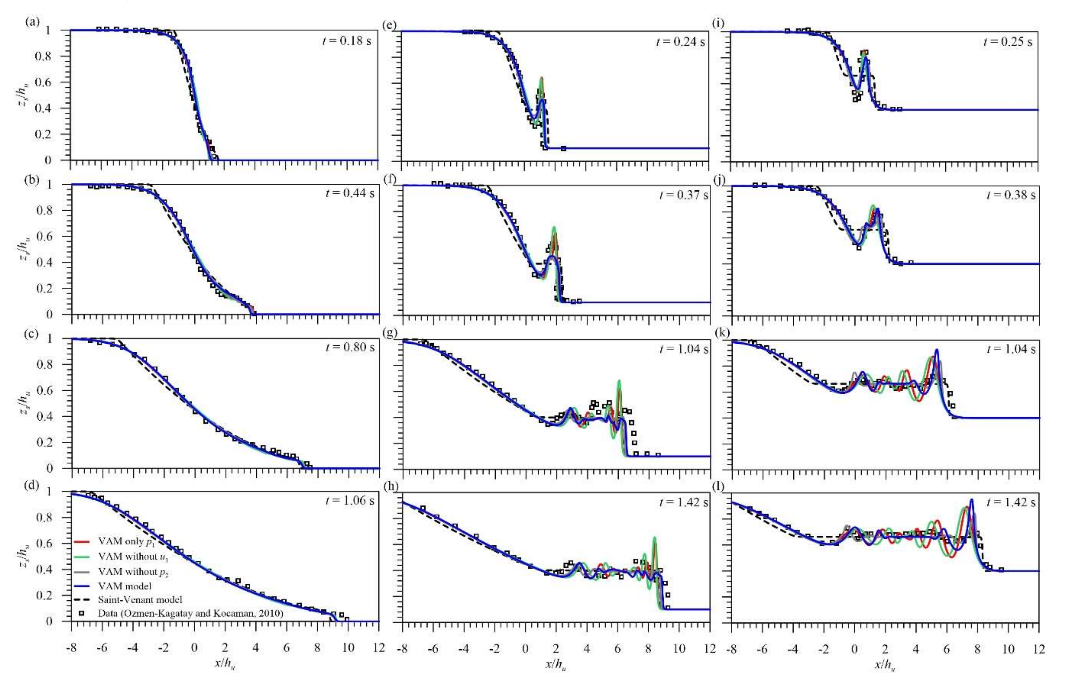
4.1. Hydrostatic versus Non-Hydrostatic Modelling

Figure 3 compares the VAM and SWE models based on [48] for r = 0 and h_u = 0.25 m, and based on [5] for r = 0.45 and h_u = 0.36 m at different times. The latter data describe an undular non-broken bore after the dam release, which is both highly non-linear and non-hydrostatic, so that these data are ideal for analyzing the importance of the non-hydrostatic effects on dam-break flow modelling. Given that no experimental data are available to describe the rarefaction wave for r = 0.45, the data for the dry downstream bed (r = 0) by [48] were also selected here for comparison purposes. The simulations were conducted by maintaining a grid step of Δx = 0.01 m and CFL = 0.1, while the bed roughness was accounted for by using n = 0.01 m^−1/3s in the turbulence closure. The ability of the VAM model to tackle the non-hydrostatic dam-break flows in both dry and wet beds with undular non-broken surges downstream is remarkable, as shown in Figure 3e–h. The dry bed front is accurately simulated by the VAM model at 0.18 s, 0.44 s, and 0.8 s (Figure 3a–c). It is somewhat delayed at 1.06 s (Figure 3d) showing an accumulative delay in the predictions that may be due to inaccuracies in the Manning’s parameter modelling. However, both the front of the undular non-broken bore and the secondary wave trains are accurately reproduced by the VAM model for r = 0.45 (Figure 3e–h). Small overestimations are observed at 0.4 s and 0.64 s (Figure 3e,f) for the peak of the advancing solitary-like wave, for which the non-linear effects are prominent. On the contrary, the SWE model fails to reproduce these highly non-hydrostatic flows. The front of the bore is overestimated for r = 0.45 (Figure 3e–h) in the SWE model, while the dry front estimated in line with the results by the VAM model for r = 0 (Figure 3a–d). For the wave train simulation for r = 0.45, only the trend of the waves is predicted (Figure 3e–h). In addition, the rarefaction wave is wrongly predicted by the SWE model, as flow curvature is not accounted for (Figure 3a–d). The non-hydrostatic modelling of dam-break flows while using depth-averaged shallow water models is, therefore, important for an accurate description of these flows. Note that non-hydrostatic effects are not important only at initiation of motion, as sometimes argued to discard non-hydrostatic modeling in practice for long simulation times. The advancing undular bore keeps its non-hydrostaticity for long simulation times, producing an evolution of the surge wave train, that ultimately tends to split in a sequence of cnoidal waves [25]. Therefore, inclusion of non-hydrostatic effects in the dam break wave modeling technology is of both theoretical and practical interest.

4.2. Simplified Non-Hydrostatic Flow Modeling

In this section, the impact of the non-hydrostatic perturbation parameters p₁ and p₂ is analyzed. To that purpose, Figure 4 shows the results of the VAM model (which accounts for both p₁ and p₂) and those of the VAM sub-model without p₂ (only accounting for p₁). They are compared to experimental data of dam-break flow over horizontal fixed bed by [48] with r = 0.4 and h_u = 0.25 m, and those by [5] with r = 0.45 and h_u = 0.1 m at different times. While the data set by [5] with r = 0.45 describes undular non-broken bores after the dam release with significant non-hydrostatic and non-linear effects, the data by [48] with r = 0.4 show the breaking of the leading wave, yielding diminished non-linear effects at the front. The simulations were conducted using Δx = 0.01 m, CFL = 0.1, and n = 0.01 m^−1/3s. The VAM models, however, fail to predict wave breaking for r = 0.4, possibly because of the oversimplified turbulence closure used, yielding, instead, solitary-like wave profile (Figure 4c–d). In line with the previous results, the VAM models accurately tackle the front of the bore and the wave train behind (Figure 4a,b,d–h) as well as the rarefaction wave (Figure 4c,d,g,h). Based on the comparison between both VAM models, it can be concluded that the impact of p₂ is minimum while modelling the non-hydrostaticity effect of dam-break flows over horizontal beds, for the selected tests. It is worth noting that, in contrast, if the bed bathymetry is uneven, p₂ is essential to tackle the free surface position [54].

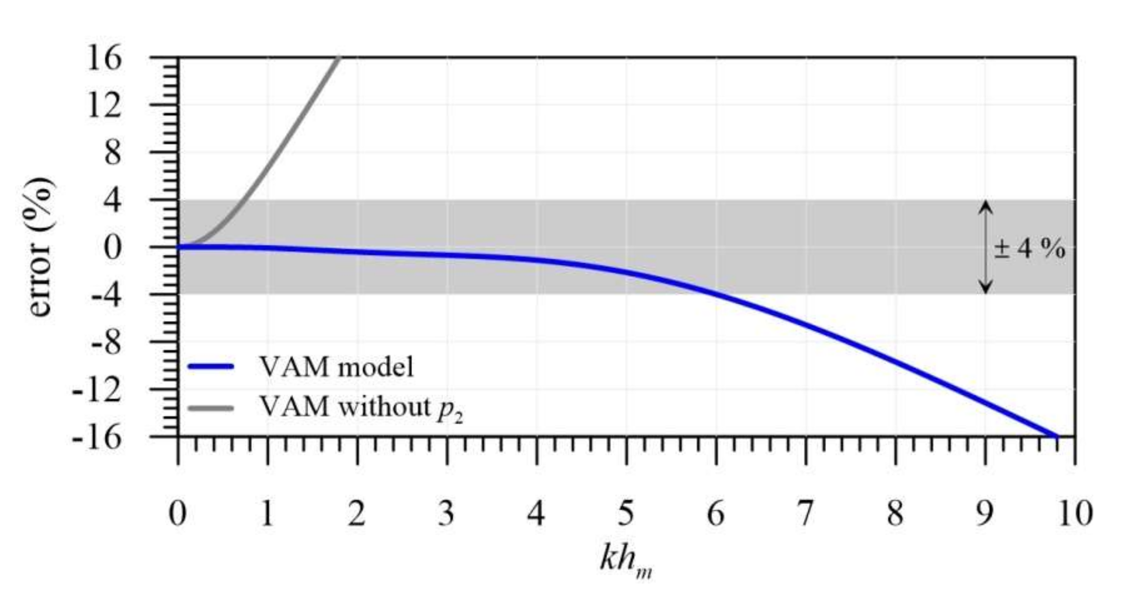
On the other hand, the exclusion of p₂ alters the frequency dispersion relation of the original VAM model. After linearization of the VAM equations, the frequency dispersion relation of the VAM model is [10,43,46]

$$\frac{c^2}{g{h}_m}=\frac{1+\frac{1}{12}{\left(k{h}_m\right)}^2}{1+\frac{5}{12}{\left(k{h}_m\right)}^2+\frac{1}{144}{\left(k{h}_m\right)}^4},$$

(19)

where c is the celerity, k the wave number, and h_m is the mean flow depth. A detailed derivation of Equation (19) is available in [46]. Eliminating p₂ from the VAM model, the corresponding dispersion relation is as follows:

$$\frac{c^2}{g{h}_m}=\frac{1+\frac{1}{12}{\left(k{h}_m\right)}^2}{1+\frac{4}{12}{\left(k{h}_m\right)}^2}.$$

(20)

Figure 5 illustrates, in relative errors, the performance of the frequency dispersion relations of the VAM model [Equation (19)] and the VAM reduced without p₂ [Equation (20)] as compared to the exact frequency dispersion relation [25], i.e., c²/gh_m = tanh(kh_m)/(kh_m). The VAM model shows a remarkable accuracy for the spectra of shallow water waves (or long waves, having kh_m << 1) and intermediate water waves (with a relative error bounded by ±4% for kh_m < 6). The VAM sub-model without p₂ provides important errors for kh_m> 0.8. Therefore, it is generally important to retain p₂, given its role in controlling the frequency dispersion at intermediate water depths.

A penalty of the VAM model as compared to the SWE relates to the computational time. In the hyperbolic step of the solver computational time of the VAM model increases as compared to that of the SWE, given that the numerical flux with the HLLC solver is computed for five PDEs instead of only two. In the elliptic step of the solver six algebraic equations are solved per cell, producing a large system of implicit equations for the whole computational domain. Computational times of VAM and SWE equations for the test by [48] with h_u = 0.25 m, h_d = 0.1 m (r = 0.4), at simulation time t = 1.04 s (T = 6.51) are compared in

Table 1. Computational times of VAM and SWE equations (seconds) using MATLAB for the test by [48] with h_u = 0.25 m, h_d = 0.1 m (r = 0.4), simulation time t = 1.04 s (T = 6.51)

∆x (m)	CFL	Full VAM Model	SWE Model
0.05	0.8	8.06	1.78
0.01	0.8	455.56	16.92
0.05	0.1	51.54	6.84
0.01	0.1	1749.98	125.58

for different time and space discretizations. For a mesh of ∆x = 0.05 m and CFL = 0.8, computational time is only a few seconds both for VAM and the SWE. Note that the MUSCL reconstruction is fourth-order accurate for both models. A reduction in CFL increases the computational time in the VAM model, but it is the reduction in ∆x which really affects the computational time. A large mesh produces stable results in the VAM model, but the accuracy in the prediction of some portions of the waves, especially the undular fronts, was inadequate, given the numerical diffusion. Therefore, ∆x was reduced and thus the number of cells increased, thereby increasing the total number of assembled equations to solve by the elliptic component of the numerical solver. This research focuses on testing the physical accuracy of the VAM model and its simplifications for dam break wave modeling rather than producing an optimized numerical solver, e.g., by resorting to a frozen Jacobian or using parallel Fortran codes. Therefore, we settled ∆x = 0.01 m and CFL = 0.1 common to all simulations, although the same accuracy in the output could be obtained with the VAM model with larger time-space discretizations in some runs. In other words, we selected discretizations to ensure accuracy for all runs, and kept this choice constant during all this research. The resulting system of the elliptic step is quite large, with typically 700 cells and 6 equations per cell, that is, 4200 unknown variables to solve in each iteration cycle of the Newton–Raphson solver. By using a frozen Jacobian matrix the computational time reported in Table 1 is easily reduced by 30%.

To the authors knowledge, this is so far the only finite-volume solver available for the VAM model. Therefore, tools for optimizing its solution are not yet available. Improvements and further developments in this regard are advisable to produce more efficient solvers.

4.3. Impact of Horizontal Velocity Modelling

In this section, the impact of modelling of the horizontal velocity field is evaluated for dam-break flow situations in which the velocity field is significantly non-uniform, such as at the breaking portion of the leading wave of the bore. To that purpose, the VAM model is compared with a VAM sub-model without u₁ using the experimental data by [48] with r = 0.1 and h_u = 0.25 m, and the data by [5] with r = 0.1 and h_u = 0.36 m. In these tests, wave breaking occurs in front of the bore after the dam release and during the subsequent instants, as shown in Figure 6. In line with Figure 3 and Figure 4, the simulations were conducted using Δx = 0.01 m, CFL = 0.1, and n = 0.01 m^−1/3s. The consideration of the linear, non-constant u-velocity profile in the VAM model by inclusion of the u₁ perturbation parameter is crucial to simulate the wave-breaking phenomenon. If u₁ were neglected, and consequently w₂ too, as already explained, the computational results of the ensuing model display highly non-linear non-breaking waves (Figure 6), similar to those obtained with Boussinesq-type models [4], in full disagreement with the experimental observations. The perturbation parameter u₁ controls the differential advection of momentum in the vertically averaged model, and thus, the dissipation needed at the wave front via velocity profile modeling to mimic wave breaking (Figure 6). In other words, the VAM model simulates the momentum velocity correction coefficient as β = 1 + 1/3(u₁/u₀)². It has been highlighted in the literature that the hydraulic approximation β = 1 is inaccurate for modeling flows with recirculation and/or significant velocity gradients [55,56,57], such as in (steady) hydraulic jumps. The broken waves simulated herein can be looked at, therefore, from the perspective of moving hydraulic jumps: the momentum flux term due to velocity profile modeling ∂/∂x[(β−1)u₀²h] partially balances the dynamic pressure terms of the x-momentum balance, namely ∂/∂x[(1/2p₁ + 2/3p₂)h/ρ], at breakers. These dynamic terms are responsible for the undulations of a surge in Boussinesq-type models, and therefore, these effects are partially suppressed at broken waves by the velocity profile modeling through the inclusion of the coefficient β. Therefore, the broken waves are significantly influenced by the velocity profile modeling, with a complex interaction between u₁, w₂, p₁, and p₂ at breakers.

This comparison shows the advantages of the VAM model over a Boussinesq-type model, namely a precise determination of non-hydrostatic pressure effects and simultaneously wave breaking, by the former. Note that wave breaking is automatically accounted for; neither a wave-breaking index is used to define its onset, as in Boussinesq-type models, nor a breaking sub-module to produce the broken fronts, as in Boussinesq-type models. Thus, relaxing the shallow water hypothesis only introducing the modeling of w and p by linear and parabolic profiles, respectively, produces a model similar to the SGNE that is still highly constrained by the unimproved assumption, namely the modeling of u(z).

The exclusion of u₁ from the VAM model also alters the frequency dispersion relation. For the VAM sub-model without u₁ (and thus also without w₂), it reads:

$$\frac{c^2}{g{h}_m}=\frac{1}{1+\frac{1}{3}{\left(k{h}_m\right)}^2}.$$

(21)

Note that the dispersion relation in Equation (20) is identical to that for the SGN equations [25] indicating that the VAM sub-model without u₁ and w₂, and the SGN equations are physically equivalent for modeling linear dispersive effects. Figure 7 shows that, in contrast with the full VAM model, excluding u₁ from the VAM model leads to significant errors, where only the shallow water waves spectrum are approximated with errors bounded by ±4%.

A complete comparison of the three data sets selected follows in the Appendix A, where, in addition, a VAM with only p₁ model is considered [8] for illustrative purposes. This reduced VAM model is also of Boussinesq-type, but based on a linear pressure profile instead of a parabolic, as with the SGNE. Since no additional insights are revealed by this model, it was excluded from the main core of the discussion presented here.

5. Conclusions

The shallow water hypotheses in dam-break flow modeling are analyzed within a vertically averaged framework using a vertically averaged and moment (VAM) equations model containing perturbation parameters introduced to overcome the limitations of the SWE.

First, the importance of considering non-hydrostatic effects was assessed by comparing the VAM model, the SWE model, and the experimental data for wet and dry bed conditions, respectively. The results reveal that the predictions by the VAM model are more accurate than those obtained with the SWE model, concluding that the inclusion of non-hydrostatic pressure effects is important to model dam-break flows.

The impact of a simplified non-hydrostatic pressure modeling was then analyzed by comparing the results of the full VAM model with those obtained by a sub-model of the VAM removing the perturbation parameter p₂. The accuracy of the sub-model for the simulations conducted was similar to that with the full VAM model, but the prediction of the frequency dispersion is inacceptable, concluding that the pressure must be modeled non-hydrostatic with a quadratic predictor.

Finally, the impact of the horizontal velocity profile modeling was quantified by comparing the full VAM model, a reduced VAM removing the variable u₁ and thus equivalent to a Boussinesq-type model, and experimental data for wet bed conditions with depth ratios producing breaking bores. The VAM sub-model without u₁ leads to non-breaking waves, as expected from Boussinesq’s theory, in full disagreement with experiments, whereas the full VAM model automatically produces broken waves. As a conclusion, it is essential to consider the horizontal velocity modeling in dam-break flows simultaneously to the non-hydrostatic pressure modeling.

SGNE and SWE correspond to extremes in the modeling of dam break waves, each having advantages and disadvantages. Only a higher-order model, such as the VAM system, has the ability of coupling simultaneously the best of both modeling technologies, by implementing non-hydrostatic pressure and velocity profile modeling. These results demonstrate that relaxing the shallow water hypotheses is important to increase the accuracy range of vertically averaged models. The VAM model via its perturbation parameters is therefore a possible tool for improving the dam-break wave modeling technology, with numerous applications in hydraulic engineering, such as the design strategies to mitigate flood hazards.