An Improved Model for Chlorophyll-a Concentration Retrieval in Coastal Waters Based on UAV-Borne Hyperspectral Imagery: A Case Study in Qingdao, China

Abstract

Chlorophyll-a (Chl-a) is an objective biological indicator, which reflects the nutritional status of coastal waters. However, the turbid coastal waters pose challenges to the application of existing Chl-a remote sensing models of case II waters. Based on the bio-optical models, we analyzed the suppression of coastal total suspended matter (TSM) on the Chl-a optical characteristics and developed an improved model using the imagery from a hyper-spectrometer mounted on an unmanned aerial vehicle (UAV). The new model was applied to estimate the spatiotemporal distribution of Chl-a concentration in coastal waters of Qingdao on 17 December 2018, 22 March 2019, and 20 July 2019. Compared with the previous models, the correlation coefficients (${\mathrm{R}}^2$) of Chl-a concentrations retrieved by the new model and in situ measurements were greatly improved, proving that the new model shows a better performance in retrieving coastal Chl-a concentration. On this basis, the spatiotemporal variations of Chl-a in Qingdao coastal waters were analyzed, showing that the spatial variation is mainly related to the TSM concentration, wind waves, and aquaculture, and the temporal variation is mainly influenced by the sea surface temperature (SST), sea surface salinity (SSS), and human activities.

1. Introduction

The ocean accounts for 71% of the Earth’s total area and has 97% of the world’s water resources. Ocean waters, especially coastal waters, are important ecosystems and provide a lot of essential ecosystem services for people. However, with the rapid development of the coastal economy, the coastal water quality has gradually deteriorated in the past decades. Especially after 1950, the development of aquaculture has led to significant degradation of the ecological environment, which has threatened biological resources and human health [1,2,3]. Since 2007, green tides have occurred in the Yellow Sea every year due to the water eutrophication caused by ocean pollution. A large amount of floating green algae attacks the coast of Qingdao, which has an adverse impact on the coastal ecological environment [4,5,6,7,8,9,10]. Chlorophyll-a (Chl-a) concentration is the most commonly used indicator to evaluate phytoplankton biomass and changes [11,12]. Variation of Chl-a concentration affects the ocean color, reflects the pollution status of ocean water, and is a critical indicator for marine environmental monitoring and assessment [13,14,15,16,17].

In the past, Chl-a concentration monitoring was based primarily on in situ measurements, which required a lot of human and material resources. Remote sensing is a very powerful tool for assessing water quality changes in coastal waters [18,19]. Hyperspectral remote sensing provides detailed spectral information for water quality assessment, but it generates considerable uncertainty in space and time, i.e., there are clear distinctions between the model structures and parameters in different regions and seasons [20,21]. The widely used spaceborne hyperspectral remote sensing provides favorable conditions for the rapid establishment of regional and seasonal models of water quality indicators. For instance, the relationship between Landsat Thematic Mapper (TM) data and suspended sediment concentration was investigated in Bernard Lake of India [22]; time-series images from the Moderate Resolution Imaging Spectroradiometer (MODIS) were used to retrieve Chl-a concentration of coastal waters at different time phases in Fujian, China [23]; charge-coupled device (CCD) images from Huanjing-1 (HJ-1) satellites and in situ Chl-a concentration obtained in Rongcheng Bay were used to verify the accuracy of three Chl-a concentration retrieval algorithms applicable to case II waters in the Yellow Sea [24]; and HJ-1 Hyper Spectral Imager (HSI) data were used to study Chl-a, total suspended matter (TSM), and turbidity in Weishan Lake of China, and an adaptive discrete binary particle swarm optimization algorithm was established [25].

However, under the current technical conditions, a high spatial resolution is difficult to achieve by spaceborne hyperspectral remote sensing, which restricts information acquisition in the spatial dimension [26]. For coastal waters, the situation is even worse, because they are independently affected by many different optical components, including Chl-a, TSM, and chromophoric dissolved organic matter (CDOM). Coastal waters have complicated spectral characteristics as well as large spectral differences in a small area [27,28]. Airborne hyperspectral remote sensing has the advantages of a high spatial resolution, high temporal resolution, and image acquisition flexibility, which provides a new method of regional water quality monitoring. Mohammad et al. summarized the commonly used airborne hyper-spectrometers for water quality monitoring. They pointed out that airborne hyperspectral sensors have a high level of flexibility in configuration and measurement time and that they are most suitable for monitoring water quality in small-scale research areas [29]. There are many studies on Chl-a concentration retrieval in small-scale waters based on airborne hyperspectral sensors [20,30,31,32,33,34]. The more commonly used airborne hyper-spectrometers include the Airborne Imaging Spectrometer for different Applications (AISA), Hyperspectral Mapper (HyMap), Airborne Visible/Near-Infrared Imaging Spectrometer (AVIRIS), and Compact Airborne Spectrographic Imager (CASI) [35]. Due to the high cost and difficulty in deployment, these sensors are often hindered. A low-cost and low-altitude hyper-spectrometer mounted on an unmanned aerial vehicle (UAV) has shown great advantages in quickly assessing the water quality of coastal or difficult-to-reach waters, and shown great value in environmental remote sensing in recent years [33].

Many research studies have been carried out on the spectral characteristics and the complex spectral interactions of various components in the seawater. A series of models for Chl-a concentration retrieval based on spectral indices have been established, which are the most widely used semi-analytical and semi-empirical models [36,37,38,39,40,41]. For case II waters in the Yellow and East China Seas, Tang et al. proposed a model called the National Satellite Ocean Application Service (NSOAS), which was developed based on the Tassan model [42,43]. The NSOAS model is particularly suitable for predicting Chl-a concentration in open-ocean waters but quickly loses its predictive powers in coastal areas [39,41]. The closer to the coast, the more complex the spectral characteristics become. As inorganic suspended matter and CDOM increase, spectral characteristics overlap each other, and the performance of the NSOAS algorithm for open-ocean waters declines [44].

In this paper, we demonstrated the process of using a UAV equipped with a hyperspectral imager to image coastal waters in Qingdao and successfully estimated the Chl-a concentration. The objective was three-fold: (1) To demonstrate the ability of UAVs equipped with hyperspectral imagers for imaging coastal waters and monitoring water quality; (2) to develop a new model to quantitatively and accurately estimate Chl-a concentration in coastal waters from UAV-borne hyperspectral radiation measurements; and (3) to analyze the spatiotemporal dynamics of Chl-a concentration according to the retrieval results on the sampling dates.

2. Materials and Methods

2.1. Study Area

The coastal waters of Qingdao are located in the southwest of the Yellow Sea; this area has a warm temperate monsoon climate. The coast is mostly composed of mountain bedrocks, and the main sediment types are silt and sandy silt. The coastal waters are mainly clean sea areas with good hydrodynamic conditions and strong self-purification ability. The deepest location is at the mouth of Jiaozhou Bay, with a water depth of about 64 m [45].

The research area is located in the coastal waters of Huangdao District in Qingdao. There are two specific areas, as shown in Figure 1: research area A and research area B. Images of the study area were acquired using the UAV-borne hyper-spectrometer on 17 December 2018, 22 March 2019, and 20 July 2019.

Images were acquired in coastal waters of northern Golden Beach (35°57′ N, 120°15′ E) in Huangdao District on 17 December 2018, i.e., research area A. Golden Beach is located in the south of Shandong peninsula, facing the Yellow Sea in the south and extending towards the southeast and is crescent-shaped. It has a total length of about 3500 m and a width of about 300 m. The water here is clear, and the sand is fine. It is a barrier-free coast formed by weathering and transformation of bedrock. There are two high and low tides every day. The annual average high tide is 3.5 m, and the average low tide is 0.9 m [46]. The primary sediments in coastal waters of northern Golden Beach are medium sands and coarse sands, so it has high visibility. There is a lot of marine life here, as well as marine farms, where one can see many fishing boats and fishers working. The long dike extending into the sea is convenient for ships to dock. There is also a broad platform on the shore for taking off and landing of UAVs equipped with hyper-spectrometers.

Images were acquired in coastal waters of northern Zhangtunzui (35°58′ N, 120°17′ E) in Huangdao District on 22 March 2019, and 20 July 2019, i.e., research area B. It is located in the south of Jiaozhou Bay mouth and north of Golden Beach, with its back against the Fenghuang Mountains. Sea erosion at an elevation of about 20 m and gentle hills at an elevation of about 50 m make up most of the coast. Tidal flats are mainly formed by shellfish deposits, and weathered and eroded bedrock gravel are deposited on lagoon beaches. Compared with the coast of Golden Beach, the hydrodynamic conditions are generally better, but there are many reefs exposed. South of the study area is close to Zhangtunzui that extends along Fenghuang mountains to the ocean, and hydrodynamic force where reef exposure is weakened, so that Enteromorpha gather easily in summer. There is also a broad platform on the shore, which is convenient for unmanned aerial vehicles (UAVs) equipped with airborne hyper-spectrometers to take off and land.

2.2. Image Data and Preprocessing

Images were acquired from a push-broom airborne hyperspectral imager named Pika L (Resonon, Inc., Bozeman, MT, USA), which covers a spectral range of 400–1000 nm with a spectral resolution of 2.1 nm. Pika L was mounted on an M600 PRO UAV (DJI, Co., Ltd., Shenzhen, Guangdong, China), and an Ellipse2-D inertial sensor (SBG Systems, S.A.S., Carrières-sur-Seine, France) was integrated to acquire orientation and position in real time during the flight, as shown in Figure 2. Before image acquisition, the flight path was planned, and flight speed and height were set using the flight control software. The flight height, speed, and sampling frame rate of hyper-spectrometer jointly determine the ground spatial resolution of the pixels on the image.

In Qingdao, hyperspectral images of coastal waters were acquired three times. The flight days are all clear and cloudless, with plenty of light and gentle wind on the shore and offshore. The flight parameters are shown in

Table 1. Flight parameters of the unmanned aerial vehicle (UAV).

Date	Flight Area	Flight Height (m)	Flight Speed (m/s)	Number of Flights	Coverage Area (m2)
17 December 2018	A	150	2.5	5	850 × 230
22 March 2019	B	200	5	3	500 × 500
20 July 2019	B	200	5	5	350 × 500

. Each of the flight tasks needed to be divided into multiple flights to cover the whole study area because of battery limitations.

Image preprocessing includes radiation calibration, atmospheric correction, image filtering, geometric correction, and flight belts mosaicking. The hyperspectral images were radiometrically calibrated to covert the digital number to radiance. Atmospheric correction was implemented on the images after radiation calibration to eliminate the influence of the atmosphere and light using the Fast Line-of-Sight Atmospheric Analysis of Spectral Hypercubes (FLAASH) module via ENVI 5.4 software (Exelis Visual Information Solutions, Inc., Boulder, CO, USA). Savitzky–Golay filtering based on local polynomial least square fitting in the time domain was adopted in this study because it can not only smooth jagged noise but also keep the basic spectral characteristics of the curves unaffected [47,48]. The flight belts were then geometrically corrected based on the principle of homography [49] and configured with geographic information according to the coordinates of imaging centers provided by the Global Positioning System (GPS) receiver connected with the Ellipse2-D sensor. All geometrically corrected flight belts were mosaicked to an image that covers the whole study area. The true color synthesis images of sea surface after preprocessing are displayed in Figure 3.

2.3. Water Sampling and Measurement

Seawater sampling and image acquisition were carried out at the same time. A total of 20, 24, and 20 water samples were collected on 17 December 2018, 22 March 2019, and 20 July 2019, respectively. The location of the sampling sites is presented in Figure 3. Because the research area is close to shore and water is shallow, sediment was easily stirred up when the ship passed. Therefore, we needed to wait for a few minutes after reaching the planned sampling sites. Surface water was collected using a 5000-mL water sampler. Water samples were injected from the water sampler into bottles and quickly frozen and stored for measurements of concentration in the laboratory.

The TSM concentration and absorption coefficient of CDOM at 440 nm were also necessary in this study. Therefore, three portions of each sample were used for collecting Chl-a, TSM, and CDOM. For Chl-a, Whatman GF/F glass microfiber filters (0.7 μm pore size) were used to filter water samples with a capacity of 2000 mL, and acetone with a volume fraction of 90% was added to extract the pigments. Chl-a concentration was determined by spectrophotometry using a Cary 5000 UV-Vis-NIR spectrophotometer (Agilent, Inc., Santa Clara, CA, USA). For TSM, water samples with a capacity of 1000 mL were filtered through Whatman cellulose acetate filters (0.45 μm pore size) and the filters were weighted gravimetrically to determine the TSM concentration. For CDOM, after the samples were filtered through Isopore membrane filters (0.2 μm pore size), the absorption coefficient of CDOM was measured in a 10-cm optical cuvette against distilled water with a Cary 5000 UV-Vis-NIR spectrophotometer. During the laboratory measurements, the test equipment was thoroughly cleaned and dried before each new sample was measured to ensure that no external pollution was introduced.

2.4. Shipborne Spectrum Sampling and Spectral Correction

To improve the quality of the sea surface spectra collected by Pika L, a shipborne marine hyperspectrometer named QE Pro (Ocean Optics, Inc., Dunedin, FL, USA) was used to automatically collect the spectra every two minutes while collecting water samples in the study area on 22 March 2019. QE Pro has a sensitivity range of 350–975 nm at an increment of 0.7 nm. It was fixed on the shipboard, measuring the radiance of skylight ($L_{sky}$), upwelling radiance from water ($L_{sw}$), and reference panel ($L_p$) according to the above-water method. The observation geometry was automatically determined by the direction of sun incidence and sea surface normal. A total of 34 spectra were obtained, as highlighted in Figure 4. In situ measurement processing included two parts: spectral preprocessing and remote sensing reflectance calculation. First, some preprocessing work (e.g., removing abnormal spectra affected by solar flares and shadows, correcting dark noise, and averaging spectra collected multiple times) was conducted to get more realistic spectra. Then, remote sensing reflectance ($R_{rs}$) was calculated according to Equation (1):

$$R_{rs}=\frac{{\rho }_p\left(L_{sw}-\delta L_{sky}\right)}{\pi L_p},$$

(1)

where ${\rho }_p$ is the irradiance reflectance of the reference panel, and $\mathsf{\delta }$ is a proportionality coefficient that relates $L_{sky}$ to the reflected sky radiance determined when the detector viewed the water surface.

Images were acquired approximately 150–200 m above the water surface using Pika L. The impact of the atmosphere between the sensor and sea surface cannot be ignored. Even if the hyperspectral images are atmospheric corrected, it still cannot represent the real sea surface reflectance. As mentioned before, a total of 34 spectra were collected by QE Pro on 22 March 2019. One of them was removed because it was located in the specular reflection area of the image, so there were 33 valid sites remaining in the dataset. Figure 5a,b display the spectral reflectance curves of 33 sites collected by Pika L and QE Pro, respectively. It can be seen that the trends of two spectral curves at the same site are similar, but the reflectance and spectral characteristics between them are different. QE Pro was closer to the sea surface than Pika L, and the observation geometry was automatically optimized. Accordingly, spectra from QE Pro can be considered more real. The spectra acquired by Pika L need to be corrected using those collected by QE Pro. Based on the coordinates of spectrum sampling sites, the differences of the reflectance from hyperspectral images and QE Pro were calculated. For each band, the least square fitting was performed on the average differences to obtain the spectral correction parameters, which were then used to correct the reflectance of images. It can not only correct the low radiance of airborne spectra due to the long observation distance but also maintain the small differences of reflectance among different sampling sites as much as possible. Figure 5c,d show the results of the least square fitting and the spectral curves of the sampling sites after correction. Considering that the differences between airborne and shipborne spectra at the same point were mainly due to factors, including the observation distance and atmospheric environment, and the distance and weather condition for each observation were basically similar, the correction parameters calculated from the 22 March 2019 observation could be used for the spectral correction of hyperspectral images acquired on 17 December 2018 and 20 July 2019.

2.5. Model Assessment

In this paper, a semi-analytical and semi-empirical algorithm was used to establish the retrieval model of Chl-a concentration. Accuracy evaluation indicators for polynomial regression were used to evaluate the algorithm, including the correlation coefficient (${\mathrm{R}}^2$), root mean square error ($\mathrm{RMSE}$), mean absolute error ($\mathrm{MAE}$), and average percentage difference ($\mathrm{APD}$). They were calculated by Equations (2)–(5), respectively:

$${\mathrm{R}}^2=\frac{{\left({{\displaystyle \sum }}_{i=1}^N\left({\left[Chla\right]}_i-\overline{\left[Chla\right]}\right)\left({\left[Chl{a}_{oc}\right]}_i-\overline{\left[Chl{a}_{oc}\right]}\right)\right)}^2}{{{\displaystyle \sum }}_{i=1}^N{\left({\left[Chla\right]}_i-\overline{\left[Chla\right]}\right)}^2{{\displaystyle \sum }}_{i=1}^N{\left({\left[Chl{a}_{oc}\right]}_i-\overline{\left[Chl{a}_{oc}\right]}\right)}^2},$$

(2)

$$\mathrm{RMSE}=\sqrt{\frac{1}{N}{{\displaystyle \sum }}_{i=1}^N{\left({\left[Chla\right]}_i-{\left[Chl{a}_{oc}\right]}_i\right)}^2},$$

(3)

$$\mathrm{MAE}=\frac{1}{N}{{\displaystyle \sum }}_{i=1}^N\left|{\left[Chla\right]}_i-{\left[Chl{a}_{oc}\right]}_i\right|,$$

(4)

$$\mathrm{APD}=\frac{1}{N}{{\displaystyle \sum }}_{i=1}^N\left|\frac{{\left[Chla\right]}_i-{\left[Chl{a}_{oc}\right]}_i}{{\left[Chla\right]}_i}\right|\times 100\%,$$

(5)

where $\left[Chla\right]$ is the concentration of in situ Chl-a, $\overline{\left[Chla\right]}$ is the average concentration of in situ Chl-a, $\left[Chl{a}_{oc}\right]$ is the concentration of retrieved Chl-a, $\overline{\left[Chl{a}_{oc}\right]}$ is the average concentration of retrieved Chl-a, $i$ represents the different sampling sites, and $N$ is the number of sampling sites.

3. Results and Discussion

3.1. Analysis of Water Samples and Spectra

Image acquisition was carried out on cloudless and sunny days. Sea surface fluctuations easily cause direct reflection of sun rays, also known as specular reflection or solar flare, appearing as a piece or scattered bright area on hyperspectral images. The water spectra of sampling sites located within the specular reflection area of images cannot represent the real reflectance and need to be eliminated. In conclusion, a valid sampling site that can be used to establish and verify the retrieval model must meet the following requirements:

• It is located within the study area covered by UAV-borne hyperspectral images after geometric correction;
• It is not located within the specular reflection area of images.

Therefore, a total of 17 valid sampling sites were obtained on 17 December 2018, 20 valid sampling sites on 22 March 2019, and 14 valid sampling sites on 20 July 2019.

Table 2. Descriptive statistics of the chlorophyll-a (Chl-a) concentrations, total suspended matter (TSM) concentrations, and absorption coefficients of chromophoric dissolved organic matter (CDOM) at water sampling sites.

Date	Number of Valid Samples	Statistics	Chl-a Concentration (mg/m3)	TSM Concentration (mg/L)	Absorption Coefficient of CDOM at 440 nm (m−1)
17 December 2018	17	Max	1.1372	11.90	0.2303
		Min	0.8409	8.48	0.0077
		Mean	1.0038	10.57	0.1418
		SD 1	0.0955	1.03	0.0593
		CV 2	9.51%	9.78%	41.85%
22 March 2019	20	Max	0.8406	27.90	0.2082
		Min	0.1007	6.20	0.1112
		Mean	0.3675	14.33	0.1625
		SD	0.2358	5.29	0.0283
		CV	64.16%	36.89%	17.42%
20 July19	14	Max	1.5477	15.74	0.1842
		Min	0.2801	5.80	0.0461
		Mean	0.6291	9.23	0.1113
		SD	0.3425	2.81	0.0378
		CV	54.44%	30.44%	33.98%

¹ SD is the standard deviation. ² CV is the coefficient of variation.

presents the descriptive statistics of the Chl-a concentrations, TSM concentrations, and absorption coefficients of CDOM at the water sampling sites.

The spectral characteristics of seawater are jointly affected by pure water, pigment particles, non-pigment particles, and CDOM [50]. In this paper, spectra were collected from the coastal waters in Qingdao with shallow water and a sandy beach. The spectral characteristics of seawater are relatively complex because of not only the water condition but also some external factors (e.g., observation geometry and illumination). According to the coordinates of the water sampling sites, the spectral curves of valid sites for three samplings were obtained from the spectral-corrected images, as shown in Figure 6.

It can be seen that the trends of the spectral curves at the wavelength of 400–800 nm are similar in different dates. The spectral characteristic is consistent with that of case II waters, but it has its uniqueness to some extent. Due to the absorption of CDOM and Chl-a, the reflectance is relatively low at the wavelength of 400–500 nm. Particularly, a valley caused by the absorption of blue-violet light by Chl-a is located at the wavelength of 420–440 nm. The absorption valley is more evident on 20 July, which is also associated with the increase of algae at this time. There is a significant reflection peak near 550 nm due to the scattering of TSM, and an unclear absorption valley of Chl-a at around 670 nm. The reflection peak appears again at the wavelength of 680–720 nm, which is generally regarded as the fluorescence peak of Chl-a. Its position is shifted to the long-wave direction as the concentration of Chl-a increases [51]. However, the high TSM concentration of coastal waters weakens the response of the fluorescence peak to the Chl-a concentration and the fluorescence peak is not significant. The peak at 750–800 nm is another reflection peak of TSM. When the concentration of TSM increases, the reflection peak will also move to the long-wave direction.

Reflectance between 400 and 800 nm is normalized to reduce the impact of external factors on the spectrum collection by the UAV-borne hyper-spectrometer and determine the sensitive bands for retrieval of the Chl-a concentration. The Pearson correlations between the normalized reflectance and Chl-a concentration or TSM concentration are demonstrated in Figure 7.

From Figure 7a, it can be concluded that there is a weak correlation between the normalized reflectance and Chl-a concentration at some bands, the most noticeable of which are the maximum positive correlation at 520–560 nm caused by the strong reflection of Chl-a at the green band and the minimum correlation at approximately 420 nm caused by the strong absorption of Chl-a at the blue-violet band. However, the correlations between the normalized reflectance and TSM concentration in different dates are not only consistent but also strong around 560 nm, as shown in Figure 7b. Overall, the correlation between Chl-a and the normalized reflectance is weaker than that between TSM and the normalized reflectance. The spectral information of seawater is dominated by a high level of TSM concentration in the coastal area of Qingdao.

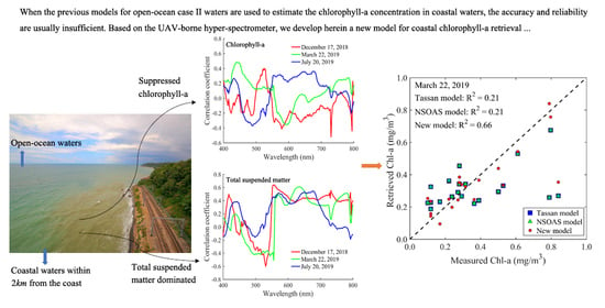
3.2. Influence of TSM on Chl-a Retrieval

In order to prove that a high TSM concentration weakens the contribution of Chl-a on the spectra in the retrieval of coastal Chl-a concentration, the bio-optical models were used to simulate the reflectance of coastal waters. The influence of pure water, CDOM, and the external environment on the reflectance was excluded, and only the interference of TSM on the retrieval of Chl-a was discussed.

The total absorption coefficient $a\left(\lambda \right)$ is expressed as a sum of the absorption coefficients for pure water $a_w\left(\lambda \right)$, Chl-a $a_{\varphi }\left(\lambda \right)$, and CDOM $a_g\left(\lambda \right)$, whereas the total backscattering coefficient $b_b\left(\lambda \right)$ is expressed as a sum of the backscattering coefficients for pure water $b_{bw}\left(\lambda \right)$, Chl-a $b_{bp}\left(\lambda \right)$, and TSM $b_{bs}\left(\lambda \right)$, as Equation (6) describes:

$$\begin{gathered} a\left(\lambda \right)=a_w\left(\lambda \right)+a_{\varphi }\left(\lambda \right)+a_g\left(\lambda \right), \\ {b}_b\left(\lambda \right)=b_{bw}\left(\lambda \right)+b_{bp}\left(\lambda \right)+b_{bs}\left(\lambda \right). \end{gathered}$$

(6)

The absorption and backscattering coefficients for pure water come from the literature [52,53]. The coefficients for other components can be simulated using the empirical models as follows [54,55,56,57]:

$$\begin{gathered} a_{\varphi }\left(\lambda \right)=\left[a_0\left(\lambda \right)+a_1\left(\lambda \right)\ln \left(0.06{\left[Chla\right]}^{0.65}\right)\right]\left(0.06{\left[Chla\right]}^{0.65}\right) \\ {a}_g\left(\lambda \right)=a_g\left(440\right)exp\left[-0.014\left(\lambda -440\right)\right] \\ {b}_{bp}\left(\lambda \right)=0.0142{\left(0.3{\left[Chla\right]}^{0.62}550/\lambda \right)}^{1.323} \\ {b}_{bs}\left(\lambda \right)=\left(0.0101\left[TSM\right]-0.0068\right){\left(532/\lambda \right)}^{0.81}, \end{gathered}$$

(7)

where $\left[Chla\right]$ and $\left[TSM\right]$ are the concentrations of Chl-a and TSM, $a_g\left(440\right)$ is the absorption coefficient of CDOM at 440 nm, $a_0\left(\lambda \right)$ and $a_1\left(\lambda \right)$ are empirical values and taken from Lee, and $\lambda$ is the wavelength.

Above-surface remote-sensing reflectance $R_{rs}\left(\lambda \right)$ can be calculated as follows [58,59]:

$$\begin{gathered} u\left(\lambda \right)=b_b\left(\lambda \right)/\left[a\left(\lambda \right)+b_b\left(\lambda \right)\right] \\ {r}_{rs}\left(\lambda \right)=\left[0.084+0.17u\left(\lambda \right)\right]u\left(\lambda \right) \\ {R}_{rs}\left(\lambda \right)=0.52r_{rs}\left(\lambda \right)/\left[1-1.7r_{rs}\left(\lambda \right)\right], \end{gathered}$$

(8)

where $u\left(\lambda \right)$ is the ratio of the backscattering coefficient to the sum of the absorption and backscattering coefficients and $r_{rs}\left(\lambda \right)$ is the subsurface remote-sensing reflectance.

The in situ measurements were substituted into the above models to simulate water reflectance, as shown in Figure 8a. The magnitude and trend of reflectance from the simulation are not completely consistent with those from the UAV-borne images because of the empirical parameters and the exclusion of the observation environment. However, the influence of changes in various parameters on remote sensing reflectance can be studied by simulation.

According to the measurements on 17 December 2018, when the TSM concentrations were set to be the reference concentration (2 mg/L), the measured minimum (~8 mg/L) and the measured maximum (~12 mg/L), the change rates of reflectance caused by the increase of Chl-a from the measured minimum (0.8409 mg/m³) to the measured maximum (1.1372 mg/m³) were simulated, as shown in Figure 8b. Similarly, Figure 8c,d show the simulations based on the measurements on 22 March 2019, and 20 July 2019, respectively. From the figures, we can see that the increase of the Chl-a concentration disturbs the water reflectance in varying degrees at varying bands. A positive change rate indicates that the water reflectance increases while the concentration of Chl-a increases, and the scattering effect of Chl-a is greater than the absorption effect. On the contrary, a negative value indicates that the absorption effect is greater than the scattering effect.

It can be seen from Figure 8b–d that when the TSM concentration is 2 mg/L and the Chl-a concentration rises (red lines), the water reflectance shows a noticeable negative rate of change between 430 and 520 nm. At this time, the absorption of Chl-a is significant. Meanwhile, the water reflectance shows a positive change after 540 nm and the scattering of Chl-a is dominant now. In particular, the change rate of reflectance is positive at 550 nm, because the reflection of Chl-a for green light is enhanced as the Chl-a concentration increases. The optical properties of water are mainly affected by Chl-a when the TSM concentration is maintained at a low level. When the TSM concentration increases to the actual level (blue and green lines), the variations of reflectance caused by the change of the Chl-a concentration become larger at the blue-green bands and smaller at the red bands, which proves that the blue and green bands are more sensitive to Chl-a concentration changes in this area. In addition, the change rate of reflectance becomes negative at 550 nm, because the contribution of Chl-a is no longer dominant due to a high level of TSM concentration. At this time, the scattering caused by the increase of Chl-a is much weaker than the TSM scattering, i.e., $u\left(\lambda \right)$ decreases, and more consideration should be given to the TSM in the retrieval.

3.3. Retrieval Model and Comparison

As we all know in the Tassan model [42], Chl-a concentration is retrieved by:

$$\lg C=c_0+c_1\lg x+c_2{\lg }^{2}x,$$

(9)

where $C$ is the retrieved concentration of Chl-a; $c_0$, $c_1$, and $c_2$ are fitting coefficients, $x=\left(R_{rs\left(443\right)}/R_{rs\left(555\right)}\right){\left(R_{rs\left(412\right)}/R_{rs\left(490\right)}\right)}^a$; $a$ is a constant related to the study area; and $R_{rs\left(i\right)}$ is the remote sensing reflectance at band $i$. The selection of bands depends on the sensitive bands of different components. The first term of $x$ is used to express the Chl-a concentration by the ratio of the absorption and reflection peak, and the second one is used to eliminate the influence of CDOM and TSM on Chl-a concentration retrieval of case II waters.

Considering that Chl-a still contributes to the spectra at the wavelength of 490 nm in the Yellow and East China Seas, the impact of TSM was removed using 510 nm instead of 490 nm, i.e., $x=\left(R_{rs\left(443\right)}/R_{rs\left(555\right)}\right){\left(R_{rs\left(412\right)}/R_{rs\left(510\right)}\right)}^a$. Therefore, the NSOAS model was proposed, which was more suitable for concentration retrieval in the Yellow and East China Seas [43].

Compared with the case II waters with a certain distance from the coast, the water is shallower and the TSM concentration is higher in coastal waters of Qingdao. The previous analysis proved that the optical properties of Chl-a are suppressed by the TSM, which causes a decline in the predictive accuracy of the Tassan and NSOAS models. Therefore, in order to improve the retrieval accuracy and further reduce the impact of TSM, two improvements were made on the NSOAS model: multiple logarithmic power of the second ratio is added to the right side of Equation (9), and ${\lg }^{2}x$ is decomposed to better reflect the concentration of Chl-a. After verification, a new retrieval model is obtained as follows:

$$\lg C=c_0+c_1\lg x_1+c_2\lg x_2+c_3{\lg }^2{x}_1+c_4{\lg }^2{x}_2+c_5\lg x_1\lg x_2+c_6{\lg }^3{x}_2+c_7{\lg }^4{x}_2,$$

(10)

where $c_0$, $c_1$, …, $c_7$ are fitting coefficients, $x_1=R_{rs\left(443\right)}/R_{rs\left(555\right)}$, and $x_2=R_{rs\left(412\right)}/R_{rs\left(510\right)}$.

Subsequently, the accuracy evaluation was performed to compare the Tassan, NSOAS, and new models, as illustrated in Figure 9. Figure 9a shows the comparison of the three models on 17 December 2018, and ${\mathrm{R}}^2$ increased from less than 0.20 to 0.65; Figure 9b shows the comparison on 22 March 2019, and ${\mathrm{R}}^2$ increased from 0.21 to 0.66; and Figure 9c shows the comparison on 20 July 2019, and ${\mathrm{R}}^2$ increased from about 0.70 to 0.79.

Table 3. Accuracy comparison for Chl-a concentration retrieval using Tassan, NSOAS, and new models on 17 December 2018, 22 March 2019, and 20 July 2019.

Date	Model	${\mathbf{R}}^2$	$\mathbf{RMSE}(\mathbf{mg}/{\mathbf{m}}^3)$	$\mathbf{MAE}(\mathbf{mg}/{\mathbf{m}}^3)$	$\mathbf{APD}(\%)$
17 December 2018	Tassan	0.17	0.08	0.07	7.49
	NSOAS	0.11	0.09	0.08	8.07
	New	0.65	0.06	0.04	4.41
22 March 2019	Tassan	0.21	0.21	0.15	49.36
	NSOAS	0.21	0.21	0.15	49.33
	New	0.66	0.14	0.09	31.84
20 July 2019	Tassan	0.71	0.18	0.15	26.05
	NSOAS	0.69	0.19	0.15	26.16
	New	0.79	0.16	0.13	21.95

summarizes the accuracy analysis of different models. It can be concluded that for the retrieval of the Chl-a concentration in the study area on 17 December 2018, 22 March 2019, and 20 July 2019, ${\mathrm{R}}^2$ of the new model was higher, and $\mathrm{RMSE}$, $\mathrm{MAE}$, and $\mathrm{APD}$ of the new model were lower than those of Tassan and NSOAS models. It is proved that the new model has higher accuracy and more advantages when applied to retrieve Chl-a concentration in coastal waters of Qingdao.

3.4. Analysis of Spatiotemporal Variation

3.4.1. Spatial Variation

The new model was applied to estimate Chl-a concentration based on the UAV-borne hyperspectral images, and the spatial distributions of Chl-a concentration on the sampling dates were obtained, as shown in Figure 10. Chl-a concentration was displayed in chromaticity. In order to demonstrate the spatial variation of Chl-a concentration in more detail, the land and retrieved outliers were excluded from the images, as well as the highest and lowest concentrations, which accounted for 5% of the total number of pixels in the study area. All excluded pixels were colored gray or white, and the remaining pixels were colored and displayed according to the concentration.

Figure 10a shows the estimated spatial distribution of Chl-a concentration in study area A on 17 December 2018. In this area, the range of Chl-a concentration was approximately 0.82–1.41 mg/m³ on this day, and the average concentration was 1.09 mg/m³. The average concentration of Chl-a is the highest of these three days. The average concentration at latitudes > 35.97° (1.13 mg/m³) is slightly higher than that at latitudes < 35.97° (1.07 mg/m³), which is mainly caused by human activities.

Figure 10b shows the estimated spatial distribution of Chl-a concentration in study area B on 22 March 2019. Affected by the marine climate, the seawater temperature reaches the lowest level of these three days, as well as the Chl-a concentration, i.e., 0.05–0.32 mg/m³, with an average concentration of 0.30 mg/m³. The lowest concentrations of Chl-a are distributed in the south of the study area, where it is close to the coast of Zhangtunzui.

Figure 10c shows the estimated spatial distribution of Chl-a concentration in study area B on 20 July 2019. On this day, the spatial changes of Chl-a are significant, ranging from 0.13 to 1.58 mg/m³. The average Chl-a concentration is about 0.72 mg/m³. The higher concentrations are distributed in the areas where algae aggregation occurs.

The distribution of Chl-a showed clear spatial variations in coastal waters of Qingdao. For study area A, a large number of fish and shrimp farms are distributed on the coast, resulting in a higher Chl-a concentration near the coast than in the distant sea on 17 December 2018. Aquaculture farms provide organic matter and nutrients to the surrounding waters, promoting the development of phytoplankton biomass, which shows the impact of human activities on the concentration of Chl-a [19,60]. For study area B, the concentration of Chl-a in the south is lower than that in the north on 22 March 2019, because the southern area is close to the coast of Zhangtunzui, and seabed sediments are deposited. A high level of TSM concentration becomes a key factor that restricts the growth of phytoplankton [24,61,62]. On 20 July 2019, the spatial changes of Chl-a concentration in this area are significant, which is related to the increase of seawater temperature and the accumulation of phytoplankton caused by wind waves [63].

3.4.2. Temporal Variation

Qingdao is located in the north extratropical monsoon climatic region, and its climatic conditions are favorable for many kinds of aquatics. Due to the influence of the southeast monsoon, ocean currents, and water masses, Qingdao has significant features of a maritime climate. It is humid, hot, and rainy in summer; the low temperature lasts for a long time in winter; and the temperature rises slowly in spring, about one month later than inland. Sea surface temperature (SST) has obvious seasonal variation characteristics, with high temperatures in summer and low temperatures in winter and spring [8]. Sea surface salinity (SSS) is mainly affected by the rainfall, and it gradually decreases from the maximum in spring with an increase of the rainfall [64,65]. Many studies have proven that the concentration of Chl-a can be influenced by various factors, such as SST, SSS, and human activities [65,66,67,68].

The Chl-a concentration in coastal waters of Qingdao has changed greatly with time. Figure 11 shows the temporal variations of the average Chl-a concentration, SST, and SSS in the study area. SST and SSS data are from the in situ measurements of the nearby Xiaomaidao ocean observation station released by the National Marine Science Data Center. As we can see from the figure, when SST decreased from 17 December to 22 March, the average Chl-a concentration also decreased. However, when SST increased drastically from 22 March to 20 July, the average Chl-a concentration also increased slightly, but it was still lower than that on December 17. It proves that SST is a critical factor that affects the concentration of Chl-a. Within a certain temperature range, the positive correlation between Chl-a concentration and SST is significant, i.e., decreasing SST will inhibit the growth of phytoplankton, and Chl-a concentration will also decrease; on the contrary, as SST increases, phytoplankton grows vigorously, and the concentration of Chl-a also increases. However, excessively high temperatures will inhibit the rise of the Chl-a concentration, which is the reason why the concentration of Chl-a on 20 July is lower than that on December 17; this finding is consistent with previous research results [69,70,71,72,73]. The change of SSS is almost the opposite of that of the Chl-a concentration. From 17 December to 22 March, SSS increased and Chl-a concentration decreased, but from 22 March to 20 July, SSS decreased and Chl-a concentration increased, showing that high salinity is a limitation for phytoplankton growth [61,65].

4. Conclusions

Considering the low predictive accuracy of the existing Chl-a concentration retrieval algorithms for case II waters, an improved retrieval algorithm for coastal waters in Qingdao was established based on UAV-borne hyperspectral images. The particularity of coastal water constituents was considered in the new algorithm, i.e., a high level of TSM concentration will suppress the optical properties of Chl-a and result in a low correlation between Chl-a concentration and spectral reflectance. Similar to the principle of the existing algorithms, the new algorithm was improved to further reduce the impact of TSM on the retrieval of Chl-a concentration. Compared with the previous algorithms, the correlation between retrieved and in situ Chl-a concentrations was higher, and the errors were lower using the new algorithm, which proved that the new algorithm was more suitable for Chl-a concentration retrieval of coastal waters.

The Chl-a concentration in the research area was estimated using the new algorithm on the sampling dates. The spatial and temporal variation characteristics of the Chl-a concentration and the relationships with various factors (e.g., SST, SSS, wind waves, and human activities) were analyzed. It is concluded that the spatial variation of Chl-a concentration in coastal waters is mainly related to the growth and reproduction of algae influenced by TSM concentration, wind waves, and aquaculture. A high level of TSM concentration will suppress the increase of Chl-a concentration, while wind waves and aquaculture will promote the rise of the Chl-a concentration of the surrounding waters. The temporal variation of the Chl-a concentration in the study area is the result of combined effects of SST, SSS, and human activities, which was the highest on December 17, followed by 20 July, and lowest on 22 March. As SST rises, phytoplankton grows vigorously and Chl-a concentration increases, but excessively high SST inhibits the rise of Chl-a concentration. Increased SSS inhibits the growth of phytoplankton, resulting in a decrease in the Chl-a concentration.

References

1. Islam, S.; Tanaka, M. Impacts of pollution on coastal and marine ecosystems including coastal and marine fisheries and approach for management: A review and synthesis. Mar. Pollut. Bull. 2004, 48, 624–649. [Google Scholar] [CrossRef] [PubMed]
2. Li, K.; Shi, X.; Bao, X.; Ma, Q.; Wang, X. Modeling total maximum allocated loads for heavy metals in Jinzhou Bay, China. Mar. Pollut. Bull. 2014, 85, 659–664. [Google Scholar] [CrossRef] [PubMed]
3. Gu, J.; Hu, C.-F.; Kuang, C.; Kolditz, O.; Shao, H.; Zhang, J.-B.; Liu, H.-X. A water quality model applied for the rivers into the Qinhuangdao coastal water in the Bohai Sea, China. J. Hydrodyn. 2016, 28, 905–913. [Google Scholar] [CrossRef]
4. Liang, Z.Y.; Lin, X.Z.; Ma, M.; Zhang, J.; Yan, X.B.; Liu, T. A preliminary study of the Enteromorpha prolifera drift gathering causing the green tide phenomenon. Period. Ocean Univ. China 2008, 38, 601–604. [Google Scholar] [CrossRef]
5. Liu, N.; Keesing, J.K.; Xing, Q.; Shi, P. World’s largest macroalgal bloom caused by expansion of seaweed aquaculture in China. Mar. Pollut. Bull. 2009, 58, 888–895. [Google Scholar] [CrossRef]
6. Liu, N.; Keesing, J.K.; Dong, Z.; Zhen, Y.; Di, B.; Shi, Y.; Fearns, P.; Shi, P. Recurrence of the world’s largest green-tide in 2009 in Yellow Sea, China: Porphyra yezoensis aquaculture rafts confirmed as nursery for macroalgal blooms. Mar. Pollut. Bull. 2010, 60, 1423–1432. [Google Scholar] [CrossRef]
7. Liu, C.-Y.; Xu, G.-B.; Deng, X.; Zhang, H.-H.; Liu, T.; Yang, G.-P. Changes in concentrations of biogenic sulfur compounds in coastal waters off Qingdao, China during an Ulva prolifera bloom. Mar. Pollut. Bull. 2020, 152, 110940. [Google Scholar] [CrossRef]
8. Miao, X.; Xiao, J.; Pang, M.; Zhang, X.; Wang, Z.; Miao, J.; Li, Y. Effect of the large-scale green tide on the species succession of green macroalgal micro-propagules in the coastal waters of Qingdao, China. Mar. Pollut. Bull. 2018, 126, 549–556. [Google Scholar] [CrossRef]
9. Shen, Q.; Li, H.; Li, Y.; Wang, Z.; Liu, J.; Yang, W. Molecular Identification of Green Algae From the Rafts Based Infrastructure of Porphyra yezoensis. Mar. Pollut. Bull. 2012, 64, 2077–2082. [Google Scholar] [CrossRef]
10. Zhang, J.; Qu, Z.; Huang, Q.; Xie, L.; Xiong, C. Solution of multiple cracks in a finite plate of an elastic isotropic material with the distributed dislocation method. Acta Mech. Solida Sin. 2014, 27, 276–283. [Google Scholar] [CrossRef]
11. McClain, C.R. A decade of satellite ocean color observations. Annu. Rev. Mar. Sci. 2009, 1, 19–42. [Google Scholar] [CrossRef] [PubMed] [Green Version]
12. Zhang, M.; Zhang, Y.; Shu, Q.; Zhao, C.; Wang, G.; Wu, Z.; Qiao, F. Spatiotemporal evolution of the chlorophyll a trend in the North Atlantic Ocean. Sci. Total. Environ. 2018, 612, 1141–1148. [Google Scholar] [CrossRef] [PubMed]
13. Kim, H.-C.; Son, S.; Kim, Y.; Khim, J.S.; Nam, J.; Chang, W.K.; Lee, J.-H.; Lee, C.-H.; Ryu, J. Remote sensing and water quality indicators in the Korean West coast: Spatio-temporal structures of MODIS-derived chlorophyll-a and total suspended solids. Mar. Pollut. Bull. 2017, 121, 425–434. [Google Scholar] [CrossRef]
14. Huang, C.; Zou, J.; Li, Y.; Yang, H.; Shi, K.; Li, J.; Wang, Y.; Chena, X.; Zheng, F. Assessment of NIR-red algorithms for observation of chlorophyll-a in highly turbid inland waters in China. ISPRS J. Photogramm. Remote Sens. 2014, 93, 29–39. [Google Scholar] [CrossRef]
15. Zhao, J.; Temimi, M.; Ghedira, H. Characterization of harmful algal blooms (HABs) in the Arabian Gulf and the Sea of Oman using MERIS fluorescence data. ISPRS J. Photogramm. Remote Sens. 2015, 101, 125–136. [Google Scholar] [CrossRef]
16. Jackson, T.; Sathyendranath, S.; Mélin, F. An improved optical classification scheme for the Ocean Colour Essential Climate Variable and its applications. Remote Sens. Environ. 2017, 203, 152–161. [Google Scholar] [CrossRef]
17. Cui, T.; Zhang, J.; Wang, K.; Wei, J.; Mu, B.; Ma, Y.; Zhu, J.; Liu, R.; Chen, X. Remote sensing of chlorophyll a concentration in turbid coastal waters based on a global optical water classification system. ISPRS J. Photogramm. Remote Sens. 2020, 163, 187–201. [Google Scholar] [CrossRef]
18. Xu, J.; Gao, C.; Wang, Y. Extraction of Spatial and Temporal Patterns of Concentrations of Chlorophyll-a and Total Suspended Matter in Poyang Lake Using GF-1 Satellite Data. Remote Sens. 2020, 12, 622. [Google Scholar] [CrossRef] [Green Version]
19. Loisel, H.; Vantrepotte, V.; Ouillon, S.; Ngoc, D.D.; Herrmann, M.; Tran, V.; Mériaux, X.; Dessailly, D.; Jamet, C.; Duhaut, T.; et al. Assessment and analysis of the chlorophyll-a concentration variability over the Vietnamese coastal waters from the MERIS ocean color sensor (2002–2012). Remote Sens. Environ. 2017, 190, 217–232. [Google Scholar] [CrossRef]
20. Pyo, J.; Ligaray, M.; Kwon, Y.S.; Ahn, M.-H.; Kim, K.; Lee, H.; Kang, T.; Cho, S.B.; Park, Y.; Cho, K.H. High-Spatial Resolution Monitoring of Phycocyanin and Chlorophyll-a Using Airborne Hyperspectral Imagery. Remote Sens. 2018, 10, 1180. [Google Scholar] [CrossRef] [Green Version]
21. Pahlevan, N.; Sarkar, S.; Franz, B. Uncertainties in coastal ocean color products: Impacts of spatial sampling. Remote Sens. Environ. 2016, 181, 14–26. [Google Scholar] [CrossRef] [PubMed]
22. Purandara, B.K.; Jamadar, B.S.; Chandramohan, T.; Jose, M.K.; Venkatesh, B. Water Quality Assessment of a Lentic Water Body Using Remote Sensing: A Case Study. In Proceedings of the Environmental Pollution; Springer Science and Business Media LLC: Berlin/Heidelberg, Germany, 2017; pp. 371–380. [Google Scholar]
23. Zhang, M.H.; Su, H.; Ji, B.W. Retrieving nearshore Chlorophyll-a concentration using MODIS time-series images in the Fujian Province (China). Acta Sci. Circumst. 2018, 38, 4831–4839. [Google Scholar] [CrossRef]
24. Sun, X.H.; Hu, L.B.; Feng, Y.L.; Pu, X.M.; Ru, S.G. Temperal and spatial analysis of chlorophyll a concentration patterns in Rongcheng Bay using HJ-1 satellite data. Transact. Ocean. Limnol. 2018, 5, 72–79. [Google Scholar] [CrossRef]
25. Cao, Y.; Ye, Y.; Zhao, H.; Jiang, Y.; Wang, H.; Shang, Y.; Wang, J. Remote sensing of water quality based on HJ-1A HSI imagery with modified discrete binary particle swarm optimization-partial least squares (MDBPSO-PLS) in inland waters: A case in Weishan Lake. Ecol. Inform. 2018, 44, 21–32. [Google Scholar] [CrossRef]
26. Pan, B.L.; Shen, H.Y.; Shao, H.; Li, W.H. Combined inversion of hyper-spectral remote sensing of space and spectrum for lake chlorophyll. J. Atmosph. Environ. Opt. 2017, 12, 428–434. [Google Scholar] [CrossRef]
27. Uudeberg, K.; Aavaste, A.; Kõks, K.-L.; Ansper, A.; Uusõue, M.; Kangro, K.; Ansko, I.; Ligi, M.; Toming, K.; Reinart, A. Optical Water Type Guided Approach to Estimate Optical Water Quality Parameters. Remote Sens. 2020, 12, 931. [Google Scholar] [CrossRef] [Green Version]
28. Le, C.; Yunmei, L.; Zha, Y.; Sun, D.; Huang, C.; Zhang, H. Remote estimation of chlorophyll a in optically complex waters based on optical classification. Remote Sens. Environ. 2011, 115, 725–737. [Google Scholar] [CrossRef]
29. Hajigholizadeh, M.; Melesse, A.M.; Reddi, L.N. Spaceborne and airborne sensors in water quality assessment. Int. J. Remote Sens. 2016, 37, 3143–3180. [Google Scholar] [CrossRef]
30. Igamberdiev, R.M.; Grenzdoerffer, G.; Bill, R.; Schubert, H.; Bachmann, M.; Lennartz, B. Determination of chlorophyll content of small water bodies (kettle holes) using hyperspectral airborne data. Int. J. Appl. Earth Obs. Geoinf. 2011, 13, 912–921. [Google Scholar] [CrossRef]
31. Johansen, R.; Beck, R.; Nowosad, J.; Nietch, C.T.; Xu, M.; Shu, S.; Yang, B.; Liu, H.; Emery, E.; Reif, M.; et al. Evaluating the portability of satellite derived chlorophyll-a algorithms for temperate inland lakes using airborne hyperspectral imagery and dense surface observations. Harmful Algae 2018, 76, 35–46. [Google Scholar] [CrossRef]
32. Olmanson, L.G.; Brezonik, P.; Bauer, M.E. Airborne hyperspectral remote sensing to assess spatial distribution of water quality characteristics in large rivers: The Mississippi River and its tributaries in Minnesota. Remote Sens. Environ. 2013, 130, 254–265. [Google Scholar] [CrossRef]
33. Shang, S.; Lee, Z.; Lin, G.; Hu, C.; Shi, L.; Zhang, Y.; Li, X.; Wu, J.; Yan, J. Sensing an intense phytoplankton bloom in the western Taiwan Strait from radiometric measurements on a UAV. Remote Sens. Environ. 2017, 198, 85–94. [Google Scholar] [CrossRef]
34. Thiemann, S.; Kaufmann, H. Lake water quality monitoring using hyperspectral airborne data—A semiempirical multisensor and multitemporal approach for the Mecklenburg Lake District, Germany. Remote Sens. Environ. 2002, 81, 228–237. [Google Scholar] [CrossRef]
35. Jia, J.; Wang, Y.; Chen, J.; Guo, R.; Shu, R.; Wang, J. Status and application of advanced airborne hyperspectral imaging technology: A review. Infrared Phys. Technol. 2020, 104, 103115. [Google Scholar] [CrossRef]
36. Gitelson, A.; Dall’Olmo, G.; Moses, W.J.; Rundquist, D.; Barrow, T.; Fisher, T.R.; Gurlin, D.; Holz, J. A simple semi-analytical model for remote estimation of chlorophyll-a in turbid waters: Validation. Remote Sens. Environ. 2008, 112, 3582–3593. [Google Scholar] [CrossRef]
37. Kutser, T.; Vahtmäe, E.; Paavel, B.; Kauer, T. Removing glint effects from field radiometry data measured in optically complex coastal and inland waters. Remote Sens. Environ. 2013, 133, 85–89. [Google Scholar] [CrossRef]
38. Yacobi, Y.Z.; Moses, W.J.; Kaganovsky, S.; Sulimani, B.; Leavitt, B.C.; Gitelson, A.A. NIR-red reflectance-based algorithms for chlorophyll-a estimation in mesotrophic inland and coastal waters: Lake Kinneret case study. Water Res. 2011, 45, 2428–2436. [Google Scholar] [CrossRef] [Green Version]
39. Moses, W.J.; A Gitelson, A.; Berdnikov, S.; Povazhnyy, V. Estimation of chlorophyll-a concentration in case II waters using MODIS and MERIS data—Successes and challenges. Environ. Res. Lett. 2009, 4, 045005. [Google Scholar] [CrossRef] [Green Version]
40. Werdell, P.J.; Bailey, S.; Franz, B.A.; Harding, L.W., Jr.; Feldman, G.C.; McClain, C.R. Regional and seasonal variability of chlorophyll-a in Chesapeake Bay as observed by SeaWiFS and MODIS-Aqua. Remote Sens. Environ. 2009, 113, 1319–1330. [Google Scholar] [CrossRef]
41. Ryan, K.; Ali, K. Application of a partial least-squares regression model to retrieve chlorophyll-a concentrations in coastal waters using hyper-spectral data. Ocean Sci. J. 2016, 51, 209–221. [Google Scholar] [CrossRef]
42. Tassan, S. Local algorithms using SeaWiFS data for the retrieval of phytoplankton, pigments, suspended sediment, and yellow substance in coastal waters. Appl. Opt. 1994, 33, 2369–2378. [Google Scholar] [CrossRef] [PubMed]
43. Tang, J.W.; Wang, X.M.; Song, Q.J.; Li, T.J.; Huang, H.J.; Ren, J.P.; Jian, W.J. Statistical inversion models for case Ⅱ water color elements in the Yellow Sea and East China Sea. Adv. Mar. Sci. 2004, 22. [Google Scholar] [CrossRef]
44. A Gitelson, A.; Gao, B.-C.; Li, R.-R.; Berdnikov, S.; Saprygin, V. Estimation of chlorophyll-a concentration in productive turbid waters using a Hyperspectral Imager for the Coastal Ocean—The Azov Sea case study. Environ. Res. Lett. 2011, 6, 024023. [Google Scholar] [CrossRef]
45. Ning, Z.; Lin, M.-M.; Zhang, Y.; Zhang, X.-B.; Kong, X.-H. Distribution of potential geological hazards and control factors in Qingdao offshore, China. China Geol. 2019, 2, 40–48. [Google Scholar] [CrossRef]
46. Yang, J.S.; Ge, Y.Z.; Wu, Q.; Wang, J.; Wang, M. Characteristics of ripples both in morphology and sediments in Golden Beach coastal zone, Huangdao and the relationship with hydrodynamics. Sci. Tech. Rev. 2014, 32, 22–29. [Google Scholar] [CrossRef]
47. Miglani, A.; Ray, S.S.; Vashishta, D.P.; Parihar, J.S. Comparison of Two Data Smoothing Techniques for Vegetation Spectra Derived From EO-1 Hyperion. J. Indian Soc. Remote Sens. 2011, 39, 443–453. [Google Scholar] [CrossRef]
48. He, Y.J.; Xie, D.H.; Zhong, R.F. Research on SG filtering algorithm based on hyperspectral image. J. Cap. Norm. Univ. (Nat. Sci. Ed.) 2018, 39, 70–75. [Google Scholar] [CrossRef]
49. Cheng, Z.G.; Zhang, L. An aerial image mosaic method based on UAV position and attitude information. Acta Geodaet. Cartogr. Sini. 2016, 45, 698–705. [Google Scholar] [CrossRef]
50. Shun, B.; Yunmei, L.; Heng, L.; Li, Z.; Meng, M.; Shaohua, L.; Jie, X.; Shuang, W.; Xiaolei, D. Estimation of chlorophyll-a concentration in Lake Erhai based on OLCI data. J. Lake Sci. 2018, 30, 701–712. [Google Scholar] [CrossRef]
51. Huang, Q.H.; He, Z.H.; Liang, H.; Yang, C.H.; Huang, F.S.; Zeng, X.B.; Li, Q.H. Estimation of chlorophyll-a concentration in Baihua Lake water based on hyspectral data. Environ. Sci. Tech. 2019, 42, 134–141. [Google Scholar] [CrossRef]
52. Pope, R.M.; Fry, E.S. Absorption spectrum (380–700 nm) of pure water II Integrating cavity measurements. Appl. Opt. 1997, 36, 8710. [Google Scholar] [CrossRef] [PubMed]
53. Morel, A. Optical properties of pure water and pure sea waters. In Proceedings of the Optical Aspects of Oceanography; Academic Press: New York, NY, USA, 1974; pp. 1–24. [Google Scholar]
54. Lee, Z.; Carder, K.L.; Mobley, C.D.; Steward, R.G.; Patch, J.S. Hyperspectral remote sensing for shallow waters. I. A semianalytical model. Appl. Opt. 1998, 37, 6329–6338. [Google Scholar] [CrossRef] [PubMed]
55. Prieur, L.; Sathyendranath, S. An optical classification of coastal and oceanic waters based on the specific spectral absorption curves of phytoplankton pigments, dissolved organic matter, and other particulate materials1. Limnol. Oceanogr. 1981, 26, 671–689. [Google Scholar] [CrossRef]
56. Bricaud, A.; Morel, A.; Prieur, L. Absorption by dissolved organic matter of the sea (yellow substance) in the UV and visible domains1. Limnol. Oceanogr. 1981, 26, 43–53. [Google Scholar] [CrossRef]
57. Song, Q.J.; Tang, J.W. The study on the scattering properties in the Huanghai Sea and East China Sea. Acta Oceanol. Sin. 2006, 28, 56–63. [Google Scholar] [CrossRef]
58. Lee, Z.; Carder, K.L.; Mobley, C.D.; Steward, R.G.; Patch, J.S. Hyperspectral remote sensing for shallow waters. 2. Deriving bottom depths and water properties by optimization. Appl. Opt. 1999, 38, 3831–3843. [Google Scholar] [CrossRef] [PubMed] [Green Version]
59. Lee, Z.; Carder, K.L.; Arnone, R.A. Deriving inherent optical properties from water color: A multiband quasi-analytical algorithm for optically deep waters. Appl. Opt. 2002, 41, 5755–5772. [Google Scholar] [CrossRef] [PubMed]
60. Li, R.; Liu, S.; Zhang, J.; Jiang, Z.; Fang, J. Sources and export of nutrients associated with integrated multi-trophic aquaculture in Sanggou Bay, China. Aquac. Environ. Interactions 2016, 8, 285–309. [Google Scholar] [CrossRef] [Green Version]
61. Sun, Y.F.; Qin, Y.J.; Li, H.B.; Wu, H. Spatial and temporal distribution characteristics and influencing factors of chlorophyll a in the Liaohe Estuary. Environ. Protec. Sci. 2020, 46, 44–48. [Google Scholar] [CrossRef]
62. Chen, J.; Liu, J. The spatial and temporal changes of chlorophyll-a and suspended matter in the eastern coastal zones of China during 1997–2013. Cont. Shelf Res. 2015, 95, 89–98. [Google Scholar] [CrossRef]
63. Nieto, K.; Mélin, F. Variability of chlorophyll-a concentration in the Gulf of Guinea and its relation to physical oceanographic variables. Prog. Oceanogr. 2017, 151, 97–115. [Google Scholar] [CrossRef] [PubMed]
64. Park, T.; Jang, C.J.; Kwon, M.; Na, H.; Kim, K.-Y. An effect of ENSO on summer surface salinity in the Yellow and East China Seas. J. Mar. Syst. 2015, 141, 122–127. [Google Scholar] [CrossRef]
65. Wang, Y.J.; Liu, Z.; Zhang, Y.; Wang, M.; Liu, D.Y. Temporal and spatial variations of chlorophyll a and environmental factors in Jiaozhou Bay in 2010–2011. Acta Oceanol. Sin. 2015, 37. [Google Scholar] [CrossRef]
66. Yang, G.P.; Jiang, T.; Zhao, Y.F.; Huang, J. Study on variation in chlorophyll a concentration and its influencing factors of Jiaozhou Bay in autumn based on long term remote sensing images. Acta Oceanol. Sin. 2019, 41, 183–190. [Google Scholar] [CrossRef]
67. Wu, X.; Duan, H.; Bi, N.; Yuan, P.; Wang, A.; Wang, H. Interannual and seasonal variation of chlorophyll-a off the Yellow River Mouth (1997–2012): Dominance of river inputs and coastal dynamics. Estuarine Coast. Shelf Sci. 2016, 183, 402–412. [Google Scholar] [CrossRef]
68. Kim, D.; Choi, S.H.; Kim, K.H.; Shim, J.; Yoo, S.; Kim, C.H. Spatial and temporal variations in nutrient and chlorophyll-a concentrations in the northern East China Sea surrounding Cheju Island. Cont. Shelf Res. 2009, 29, 1426–1436. [Google Scholar] [CrossRef]
69. Ji, C.; Zhang, Y.; Qiuming, C.; Tsou, J.; Jiang, T.; Liang, X.S. Evaluating the impact of sea surface temperature (SST) on spatial distribution of chlorophyll-a concentration in the East China Sea. Int. J. Appl. Earth Obs. Geoinf. 2018, 68, 252–261. [Google Scholar] [CrossRef]
70. Nurdin, S.; Mustapha, M.A.; Lihan, T. The relationship between sea surface temperature and chlorophyll-a concentration in fisheries aggregation area in the archipelagic waters of spermonde using satellite images. In Proceedings of the the 2013 UKM FST POSTGRADUATE COLLOQUIUM, Proceedings of the Universiti Kebangsaan Malaysia, Faculty of Science and Technology 2013 Postgraduate Colloquium, Selangor, Malaysia, 3–4 July 2013; AIP Publishing: College Park, MD, USA, 2013; pp. 466–472. [Google Scholar]
71. Suchenwirth, L.; Förster, M.; Cierjacks, A.; Lang, F.; Kleinschmit, B. Knowledge-based classification of remote sensing data for the estimation of below- and above-ground organic carbon stocks in riparian forests. Wetl. Ecol. Manag. 2012, 20, 151–163. [Google Scholar] [CrossRef]
72. Shi, F.; Cui, L.; Jiang, H.Z.; Shen, Y.M. Numerical analysis of the effects of seasonal variation on distributions and influences of surface chlorophyll-a in the Yellow Sea and the Bohai Sea. J. Bas. Sci. Engin. 2017, 25, 700–711. [Google Scholar] [CrossRef]
73. Zhao, N.; Zhang, G.; Zhang, S.; Bai, Y.; Ali, S.; Zhang, J. Temporal-Spatial Distribution of Chlorophyll-a and Impacts of Environmental Factors in the Bohai Sea and Yellow Sea. IEEE Access 2019, 7, 160947–160960. [Google Scholar] [CrossRef]
Figure 1. Location of the study areas. Research areas A and B are marked with black solid squares.
Water 12 02769 g001
Figure 2. (a) The M600 PRO unmanned aerial vehicle (UAV) equipped with the Pika L; (b) the Pika L with the integrated Ellipse2-D inertial sensor.
Water 12 02769 g002
Figure 3. Hyperspectral true color synthesis images of sea surface after preprocessing on (a) 17 December 2018, (b) 22 March 2019, and (c) 20 July 2019. Red dots denote water sampling sites, and the red box denotes the fifth flight on 17 December 2018.
Water 12 02769 g003
Figure 4. Location of the spectrum sampling sites. The yellow dots are the sites for spectrum collection by QE Pro on 22 March 2019.
Water 12 02769 g004
Figure 5. Reflectance spectra from spectrum sampling sites obtained by (a) Pika L and (b) QE Pro; (c) least square fitting of the mean differences between shipborne and airborne spectra; and (d) spectra after spectral correction.
Water 12 02769 g005
Figure 6. Reflectance spectra after spectral correction at water sampling sites on (a) 17 December 2018, (b) 22 March 2019, and (c) 20 July 2019.
Water 12 02769 g006
Figure 7. Pearson correlation coefficients (a) between normalized reflectance and Chl-a concentration; (b) between normalized reflectance and TSM concentration.
Water 12 02769 g007
Figure 8. (a) The simulated water reflectance by the bio-optical models based on the measurements and empirical parameters; the change rates of the water reflectance when Chl-a concentrations rise from the measured minimum to the measured maximum with different total suspended matter (TSM) concentrations: (b) from 0.8409 to 1.1372 mg/m3 on 17 December 2018; (c) from 0.1007 to 0.8406 mg/m3 on 22 March 2019; (d) from 0.2801 to 1.5477 mg/m3 on 20 July 2019.
Water 12 02769 g008
Figure 9. Comparison of in situ measured Chl-a concentrations and retrieved Chl-a concentrations by Tassan, National Satellite Ocean Application Service (NSOAS), and the new models: (a) comparison for 17 December 2018; (b) comparison for 22 March 2019; and (c) comparison for 20 July 2019.
Water 12 02769 g009
Figure 10. The estimated spatial distributions of Chl-a concentrations in the study areas on (a) 17 December 2018, (b) 22 March 2019, and (c) 20 July 2019.
Water 12 02769 g010
Figure 11. The temporal variations of average Chl-a concentration, sea surface temperature (SST), and sea surface salinity (SSS), and the relationship between them.
Water 12 02769 g011