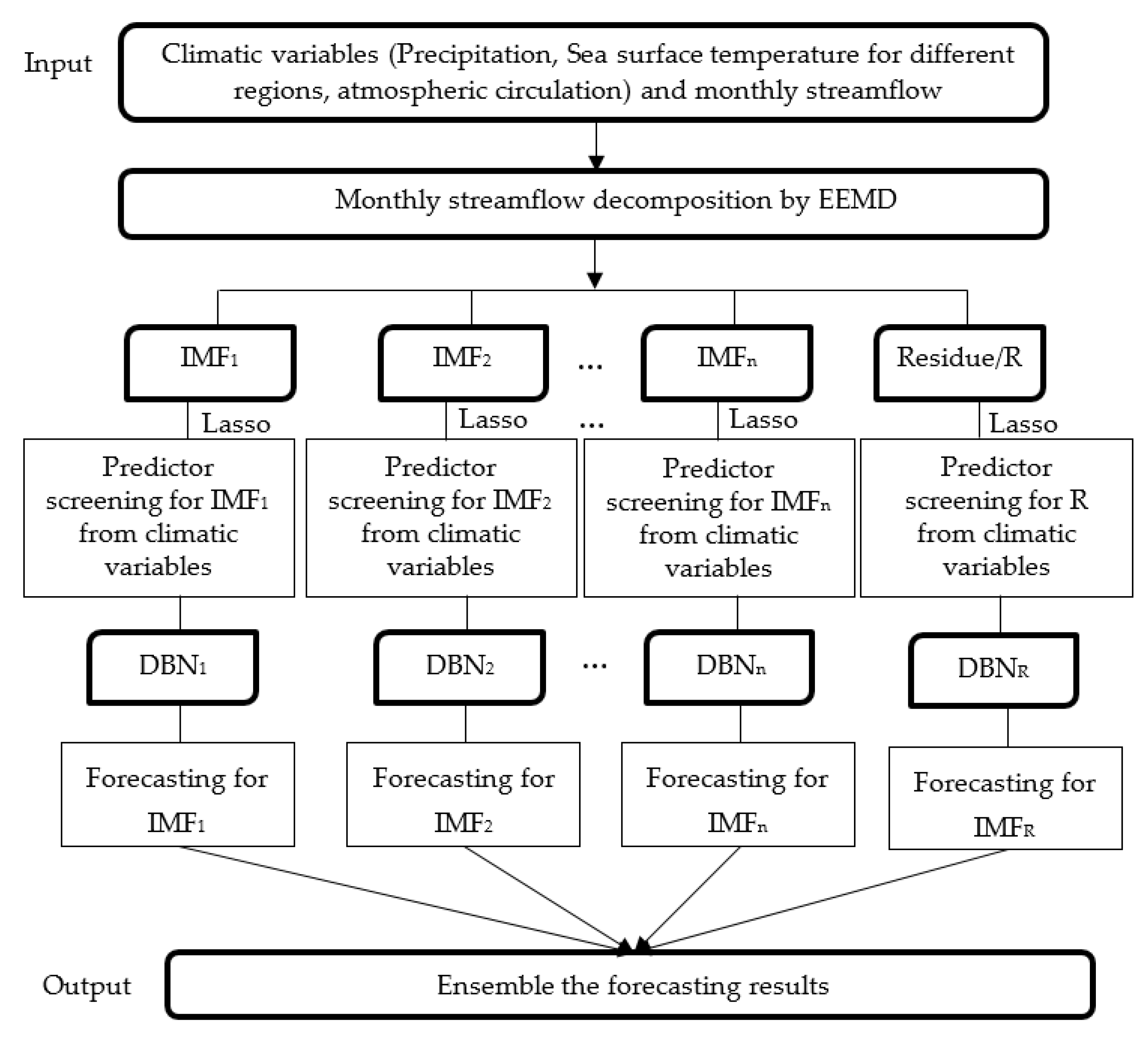
Monthly Streamflow Forecasting Using EEMD-Lasso-DBN Method Based on Multi-Scale Predictors Selection


Abstract
:1. Introduction
2. Materials and Methods
2.1. Ensemble Empirical Mode Decomposition (EEMD)
2.2. Least Absolute Shrinkage and Selection Operator (Lasso)
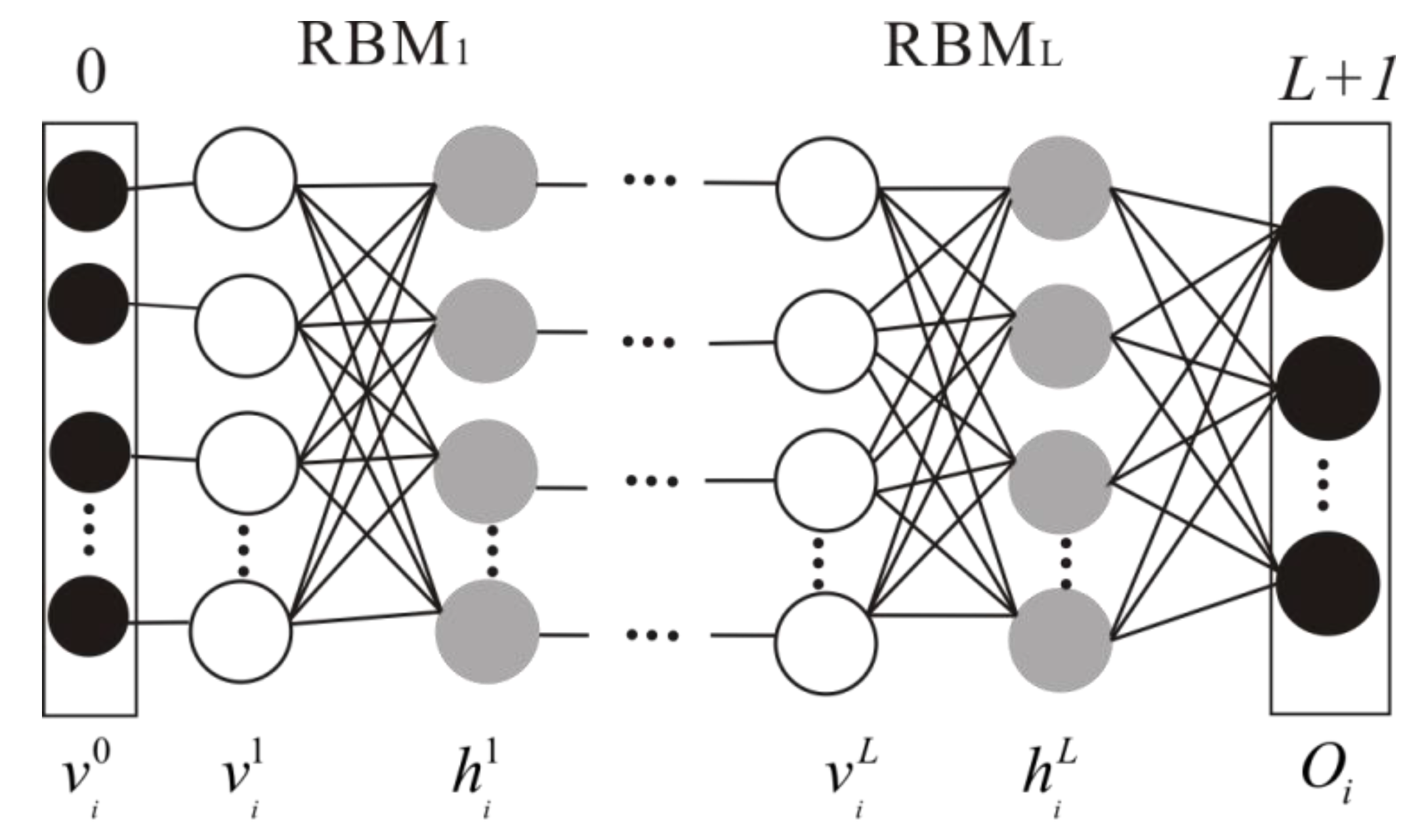
2.3. Deep Belief Networks (DBN)
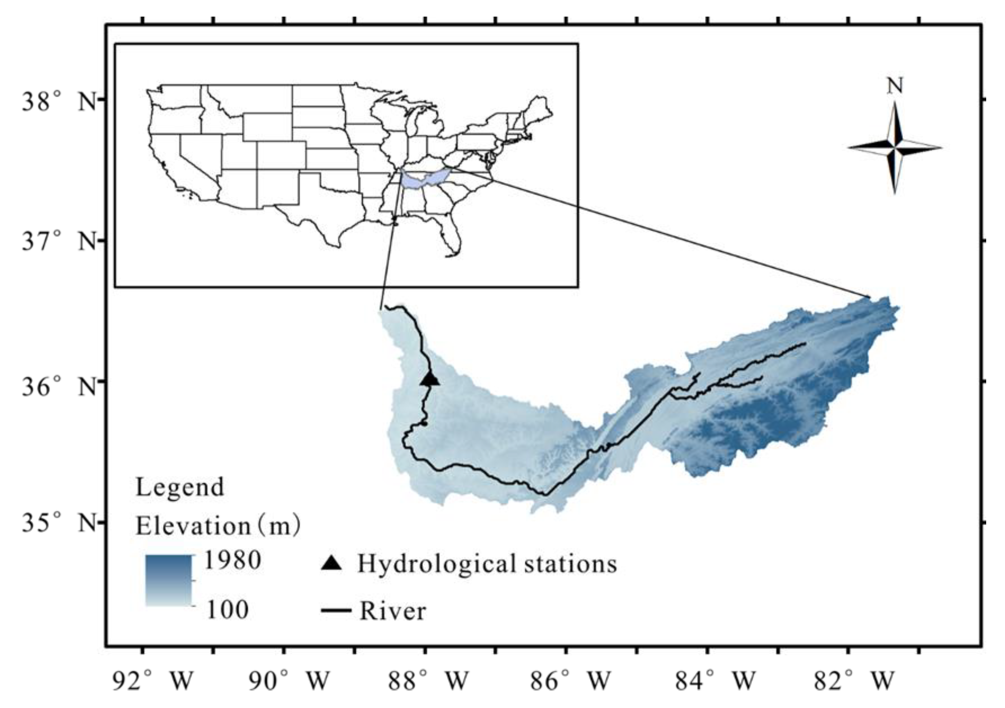
3. Study Area and Data
3.1. Study Area
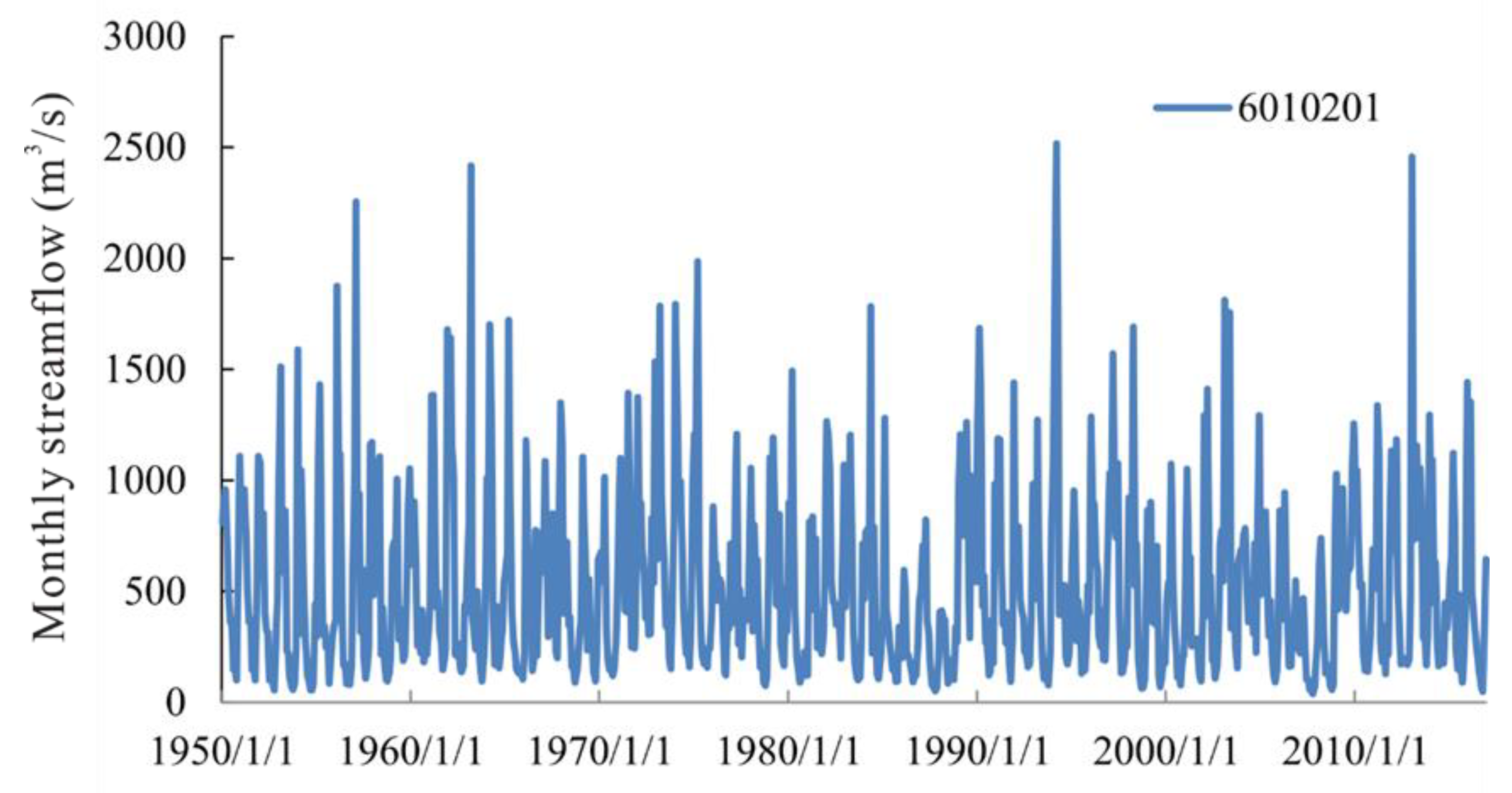
3.2. Data
4. Results and Discussion
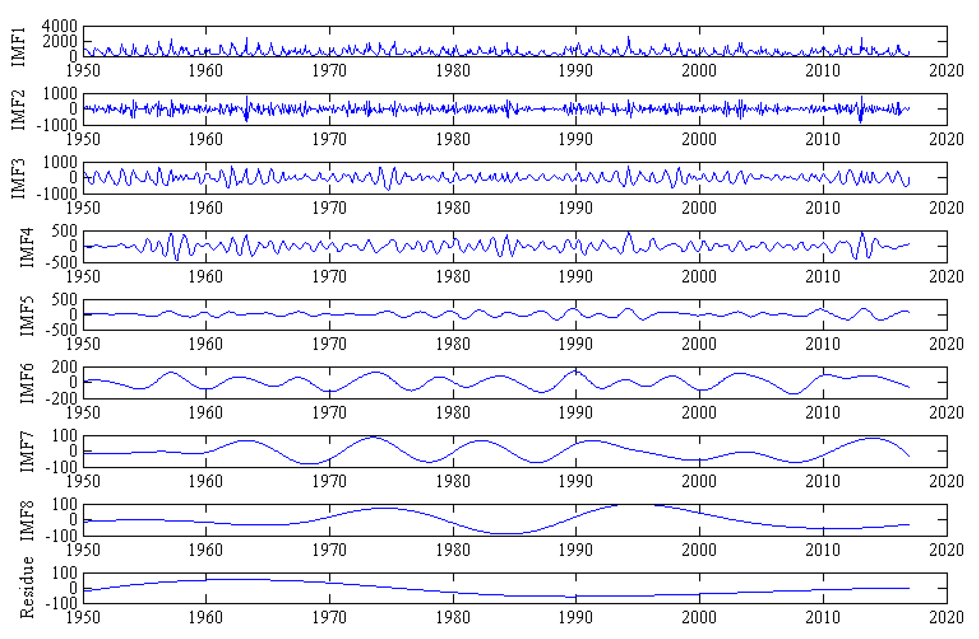
4.1. Investigation of Main Elements Decomposition
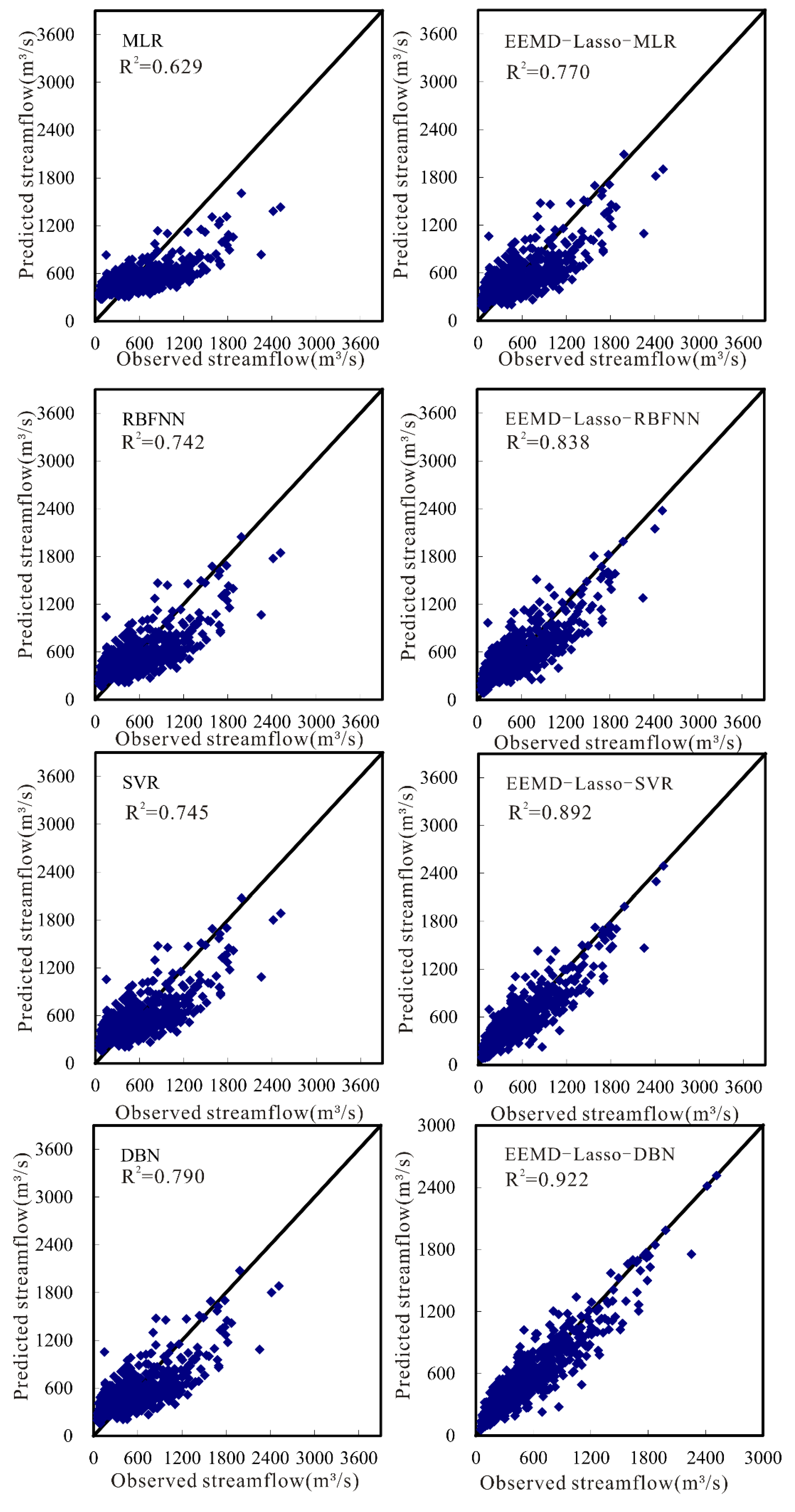
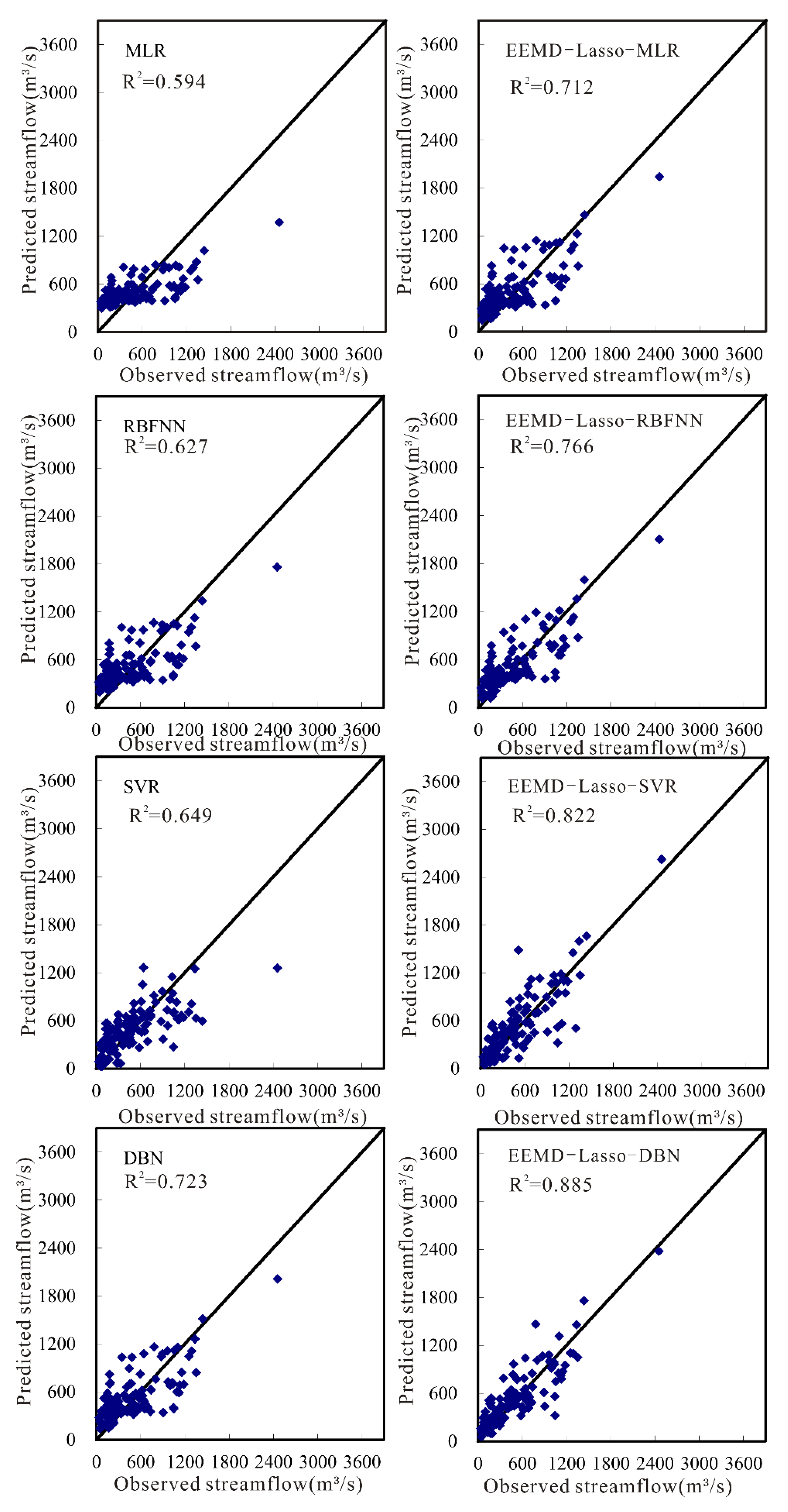
4.2. Investigation of Different Forecasting Methods
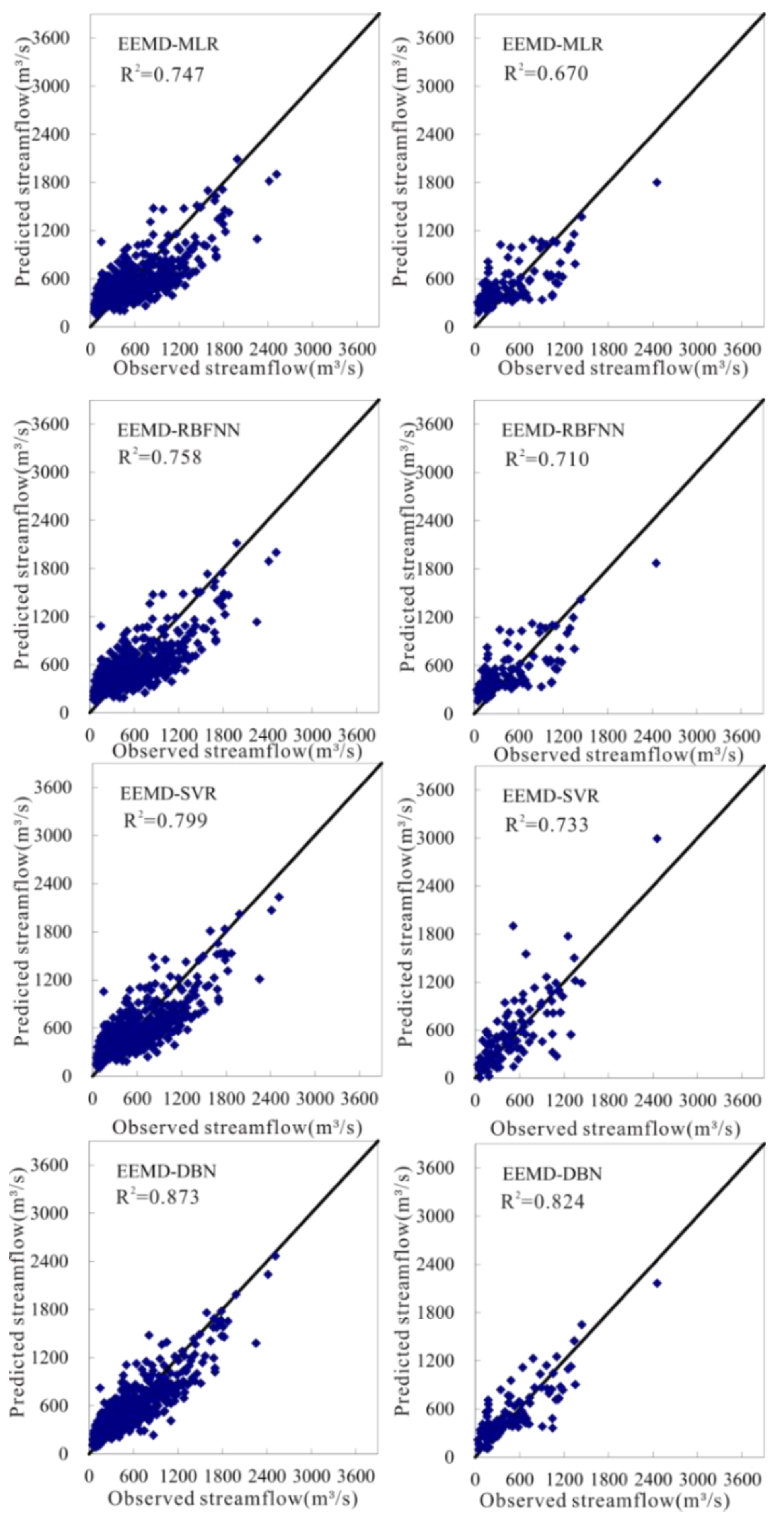
4.3. Investigation of the Forecasting Models with EEMD
4.4. Investigation of the Forecasting Models with EEMD and Lasso
5. Conclusions
Author Contributions
Funding
Acknowledgments
Conflicts of Interest
References
- Carrier, C.; Kalra, A.; Ahmad, S. Using paleo reconstructions to improve streamflow forecast lead time in the western United States. J. Am. Water Resour. Assoc. 2013, 49, 1351–1366. [Google Scholar] [CrossRef]
- Anghileri, D.; Voisin, N.; Castelletti, A.; Pianosi, F.; Nijssen, B.; Lettenmaier, D.P. Value of long-term streamflow forecasts to reservoir operations for water supply in snow-dominated river catchments. Water Resour. Res. 2016, 52, 4209–4225. [Google Scholar] [CrossRef] [Green Version]
- Zhang, Y.; Lian, J.; Liu, F. An improved filtering method based on EEMD and wavelet-threshold for modal parameter identification of hydraulic structure. Mech. Syst. Signal Process. 2016, 68, 316–329. [Google Scholar] [CrossRef]
- Wood, A.W.; Hopson, T.; Newman, A.; Brekke, L.; Arnold, J.; Clark, M. Quantifying streamflow forecast skill elasticity to initial condition and climate prediction skill. J. Hydrometeorol. 2016, 17, 651–668. [Google Scholar] [CrossRef]
- Opitz-Stapleton, S.; Gangopadhyay, S.; Rajagopalan, B. Generating streamflow forecasts for the Yakima River Basin using large-scale climate predictors. J. Hydrol. 2007, 341, 131–143. [Google Scholar] [CrossRef]
- Amigo, J.M.; Gredilla, A.; de Vallejuelo, S.F.O.; de Diego, A.; Madariaga, J.M. Study of parameters affecting the behaviour of trace elements in a polluted estuary. Canonical correlation analysis as a tool in environmental impact assessment. Chemom. Intell. Lab. 2012, 119, 1–10. [Google Scholar] [CrossRef]
- Risko, S.L.; Martinez, C.J. Forecasts of seasonal streamflow in West-Central Florida using multiple climate predictors. J. Hydrol. 2014, 519, 1130–1140. [Google Scholar] [CrossRef]
- McNeish, D.M. Using lasso for predictor selection and to assuage overfitting: A method long overlooked in behavioral sciences. Multivar. Behav. Res. 2015, 50, 471–484. [Google Scholar] [CrossRef] [PubMed]
- Liu, Z.; Sun, W.; Zeng, J. A new short-term load forecasting method of power system based on EEMD and SS-PSO. Neural Comput. Appl. 2014, 24, 973–983. [Google Scholar] [CrossRef]
- Kasiviswanathan, K.S.; He, J.; Sudheer, K.P.; Tay, J.H. Potential application of wavelet neural network ensemble to forecast streamflow for flood management. J. Hydrol. 2016, 536, 161–173. [Google Scholar] [CrossRef]
- Wu, C.L.; Chau, K.W.; Li, Y.S. Predicting monthly streamflow using data-driven models coupled with data-preprocessing techniques. Water Resour. Res. 2009, 45, 8. [Google Scholar] [CrossRef]
- Zhang, X.; Peng, Y.; Zhang, C.; Wang, B. Are hybrid models integrated with data preprocessing techniques suitable for monthly streamflow forecasting? Some experiment evidences. J. Hydrol. 2015, 530, 137–152. [Google Scholar] [CrossRef]
- Mehr, A.D.; Kahya, E. A Pareto-optimal moving average multigene genetic programming model for daily streamflow prediction. J. Hydrol. 2017, 549, 603–615. [Google Scholar] [CrossRef]
- Lee, H.S. Estimation of extreme sea levels along the Bangladesh coast due to storm surge and sea level rise using EEMD and EVA. J. Geophys. Res. Ocean. 2013, 118, 4273–4285. [Google Scholar] [CrossRef] [Green Version]
- Fu, W.; Zhou, J.; Zhang, Y.; Zhu, W.; Xue, X.; Xu, Y. A state tendency measurement for a hydro-turbine generating unit based on aggregated EEMD and SVR. Meas. Sci. Technol. 2015, 26, 125008. [Google Scholar] [CrossRef]
- Zhang, H.; Singh, V.P.; Wang, B.; Yu, Y. CEREF: A hybrid data-driven model for forecasting annual streamflow from a socio-hydrological system. J. Hydrol. 2016, 540, 246–256. [Google Scholar] [CrossRef]
- Wang, W.; Van Gelder, P.H.; Vrijling, J.K.; Ma, J. Forecasting daily streamflow using hybrid ANN models. J. Hydrol. 2006, 324, 383–399. [Google Scholar] [CrossRef]
- Tootle, G.A.; Singh, A.K.; Piechota, T.C.; Farnham, I. Long lead-time forecasting of US streamflow using partial least squares regression. J. Hydrol. Eng. 2007, 12, 442–451. [Google Scholar] [CrossRef]
- Ausati, S.; Amanollahi, J. Assessing the accuracy of ANFIS, EEMD-GRNN, PCR, and MLR models in predicting PM 2.5. Atmos. Environ. 2016, 142, 465–474. [Google Scholar] [CrossRef]
- Solomatine, D.P.; Xue, Y. M5 model trees and neural networks: Application to flood forecasting in the upper reach of the Huai River in China. J. Hydrol. Eng. 2004, 9, 491–501. [Google Scholar] [CrossRef]
- Wang, W.C.; Chau, K.W.; Qiu, L.; Chen, Y.B. Improving forecasting accuracy of medium and long-term runoff using artificial neural network based on EEMD decomposition. Environ. Res. 2015, 139, 46–54. [Google Scholar] [CrossRef] [PubMed]
- Shao, H.; Jiang, H.; Wang, F.; Wang, Y. Rolling bearing fault diagnosis using adaptive deep belief network with dual-tree complex wavelet packet. ISA Trans. 2017, 69, 187–201. [Google Scholar] [CrossRef] [PubMed]
- Huang, N.E.; Wu, Z. A review on Hilbert-Huang transform: Method and its applications to geophysical studies. Rev. Geophys. 2008, 46, 2. [Google Scholar] [CrossRef]
- Hawinkel, P.; Swinnen, E.; Lhermitte, S.; Verbist, B.; Van Orshoven, J.; Muys, B. A time series processing tool to extract climate-driven interannual vegetation dynamics using ensemble empirical mode decomposition (EEMD). Remote Sens. Environ. 2015, 169, 375–389. [Google Scholar] [CrossRef] [Green Version]
- Ouyang, Q.; Lu, W.; Xin, X.; Zhang, Y.; Cheng, W.; Yu, T. Monthly rainfall forecasting using EEMD-SVR based on phase-space reconstruction. Water Resour. Manag. 2016, 30, 2311–2325. [Google Scholar] [CrossRef]
- Barge, J.T.; Sharif, H.O. An ensemble empirical mode decomposition, self-organizing map, and linear genetic programming approach for forecasting river streamflow. Water 2016, 8, 2016247. [Google Scholar] [CrossRef]
- Zang, H.; Fan, L.; Guo, M.; Wei, Z.; Sun, G.; Zhang, L. Short-Term Wind Power Interval Forecasting Based on an EEMD-RT-RVM Model. Adv. Meteorol. 2016, 2016, 1–10. [Google Scholar] [CrossRef]
- Wang, W.C.; Xu, D.M.; Chau, K.W.; Chen, S. Improved annual rainfall-runoff forecasting using PSO–SVM model based on EEMD. J. Hydroinform. 2013, 15, 1377–1390. [Google Scholar] [CrossRef]
- Peng, T.; Zhou, J.; Zhang, C.; Fu, W. Streamflow forecasting using empirical wavelet transform and artificial neural networks. Water. 2017, 9, 406. [Google Scholar] [CrossRef]
- Guo, Z.; Zhao, W.; Lu, H.; Wang, J. Multi-step forecasting for wind speed using a modified EMD-based artificial neural network model. Renew. Energy 2012, 37, 241–249. [Google Scholar] [CrossRef]
- Zou, H. The adaptive lasso and its oracle properties. J. Am. Stat. Assoc. 2006, 101, 1418–1429. [Google Scholar] [CrossRef]
- Nardi, Y.; Rinaldo, A. Autoregressive process modeling via the lasso procedure. J. Multivar. Anal. 2011, 102, 528–549. [Google Scholar] [CrossRef]
- Kwon, S.; Lee, S.; Na, O. Tuning parameter selection for the adaptive Lasso in the autoregressive model. J. Korean Stat. Soc. 2017, 46, 285–297. [Google Scholar] [CrossRef]
- Chen, H.; Wang, J.; Tang, B.; Xiao, K.; Li, J. An integrated approach to planetary gearbox fault diagnosis using deep belief networks. Meas. Sci. Technol. 2016, 28, 025010. [Google Scholar] [CrossRef]
- Zhang, R.; Shen, F.; Zhao, J. A model with fuzzy granulation and deep belief networks for exchange rate forecasting. In Proceedings of the 2014 International Joint Conference on Neural Networks (IJCNN), Beijing, China, 6–11 July 2014; pp. 366–373. [Google Scholar]
- Chen, J.; Jin, Q.; Chao, J. Design of deep belief networks for short-term prediction of drought index using data in the Huaihe river basin. Math. Probl. Eng. 2012, 2012, 1–16. [Google Scholar] [CrossRef]
- Dedinec, A.; Filiposka, S.; Dedinec, A.; Kocarev, L. Deep belief network based electricity load forecasting: An analysis of Macedonian case. Energy 2016, 115, 1688–1700. [Google Scholar] [CrossRef]
- Chen, Z.; Li, W. Multisensor Feature Fusion for Bearing Fault Diagnosis Using Sparse Autoencoder and Deep Belief Network. IEEE Trans. Instrum. Meas. 2017, 66, 1693–1702. [Google Scholar] [CrossRef]
- Zhong, P.; Gong, Z.; Li, S.; Schönlieb, C.B. Learning to Diversify Deep Belief Networks for Hyperspectral Image Classification. IEEE Trans. Geosci. Remote. 2017, 55, 3516–3530. [Google Scholar] [CrossRef]
- Agana, N.A.; Homaifar, A. EMD-Based Predictive Deep Belief Network for Time Series Prediction: An Application to Drought Forecasting. Hydrology 2018, 5, 18. [Google Scholar] [CrossRef]
- Yang, H.; Hu, B.; Pan, X.; Yan, S.; Feng, Y.; Zhang, X.; Yin, L.; Hu, C. Deep belief network-based drug identification using near infrared spectroscopy. J. Innov. Opt. Health Sci. 2017, 10, 1630011. [Google Scholar] [CrossRef]


| Data | Predictors |
|---|---|
| IMF1 | rainfall |
| IMF2 | rainfall, SST3, SST4, SST6, SST7, SST10 |
| IMF3 | rainfall, SST1, SST5, SST6, SST7, SST8, SST10 |
| IMF4 | rainfall |
| IMF5 | rainfall |
| IMF6 | rainfall, AO, PNA, PDO, NAO, NINO3, SST3, SST6, SST7, SST10 |
| IMF7 | rainfall, AO, PDO, NAO, SOI, NINO3, NINO3.4, SST1-4, SST6, SST10 |
| IMF8 | rainfall, AO, PDO, NAO, SOI, NINO3, NINO4, NINO3.4, SST1-3, SST6-10 |
| Residue | AO, PNA, PDO, SOI, NINO3, NINO4, NINO3.4, SST1-3, SST6-10 |
| Model Calibration | Model Validation | |||||||
|---|---|---|---|---|---|---|---|---|
| MAE | RMSE | NS | R2 | MAE | RMSE | NS | R2 | |
| MLR | 0.848 | 310 | 0.420 | 0.629 | 1.09 | 308 | 0.400 | 0.594 |
| RBFNN | 0.741 | 278 | 0.534 | 0.742 | 0.965 | 287 | 0.479 | 0.627 |
| SVR | 0.730 | 275 | 0.542 | 0.745 | 0.952 | 286 | 0.483 | 0.649 |
| DBN | 0.637 | 251 | 0.618 | 0.790 | 0.841 | 268 | 0.546 | 0.723 |
| Model Calibration | Model Validation | |||||||
|---|---|---|---|---|---|---|---|---|
| MAE | RMSE | NS | R2 | MAE | RMSE | NS | R2 | |
| EEMD-MLR | 0.725 | 274 | 0.546 | 0.747 | 0.945 | 285 | 0.485 | 0.670 |
| EEMD-RBFNN | 0.699 | 268 | 0.566 | 0.758 | 0.913 | 282 | 0.498 | 0.710 |
| EEMD-SVR | 0.620 | 247 | 0.632 | 0.799 | 0.821 | 264 | 0.560 | 0.733 |
| EEMD-DBN | 0.462 | 202 | 0.754 | 0.873 | 0.631 | 221 | 0.691 | 0.824 |
| Model Calibration | Model Validation | |||||||
|---|---|---|---|---|---|---|---|---|
| MAE | RMSE | NS | R2 | MAE | RMSE | NS | R2 | |
| EEMD-Lasso-MLR | 0.674 | 261 | 0.586 | 0.770 | 0.884 | 277 | 0.515 | 0.712 |
| EEMD-Lasso-RBFNN | 0.544 | 225 | 0.694 | 0.838 | 0.728 | 243 | 0.627 | 0.766 |
| EEMD-Lasso-SVR | 0.413 | 187 | 0.788 | 0.892 | 0.580 | 210 | 0.722 | 0.822 |
| EEMD-Lasso-DBN | 0.245 | 158 | 0.848 | 0.922 | 0.427 | 189 | 0.775 | 0.885 |
© 2018 by the authors. Licensee MDPI, Basel, Switzerland. This article is an open access article distributed under the terms and conditions of the Creative Commons Attribution (CC BY) license (http://creativecommons.org/licenses/by/4.0/).
Share and Cite
Chu, H.; Wei, J.; Qiu, J. Monthly Streamflow Forecasting Using EEMD-Lasso-DBN Method Based on Multi-Scale Predictors Selection. Water 2018, 10, 1486. https://doi.org/10.3390/w10101486
Chu H, Wei J, Qiu J. Monthly Streamflow Forecasting Using EEMD-Lasso-DBN Method Based on Multi-Scale Predictors Selection. Water. 2018; 10(10):1486. https://doi.org/10.3390/w10101486
Chicago/Turabian StyleChu, Haibo, Jiahua Wei, and Jun Qiu. 2018. "Monthly Streamflow Forecasting Using EEMD-Lasso-DBN Method Based on Multi-Scale Predictors Selection" Water 10, no. 10: 1486. https://doi.org/10.3390/w10101486