Evaluation of Water Scarcity in Selected Countries of the Middle East

Abstract

The primary goal of this article is to evaluate water scarcity in selected countries of the Middle-East and assess the impact on agricultural production. To begin with, the Weighted Anomaly Standardized Precipitation (WASP) Index from 1979 to 2017 was spatially computed for Iran, Iraq and Saudi Arabia. In order to demonstrate the effect of reduced levels of water, the water shortage situation in cities with the population higher than one million was examined. This was accomplished by utilizing the Composite Index approach to make water related statistics more intelligible. A projection for the years of 2020 to 2030 was created in order to demonstrate possible changes in the supply and demand for water in selected countries of the Middle-East. In regards to evaluating the economic effects of water shortages on agricultural sector, effects of lower precipitation on agricultural production in Iran, Iraq and Saudi Arabia were estimated. With ever-increasing urbanization, all countries are currently experiencing a moderate to high water risk. Our research points to excessively high water stress for most analyzed cities through the year 2030. Also, it is demonstrated how much precipitation decreases influence agricultural production in Iran, Iraq and Saudi Arabia. From the analyzed countries, some evidence is found that precipitation negatively influences crop production, primarily for Iran.

1. Introduction

Water scarcity refers to long-term water imbalances, combining low water availability with a level of water demand exceeding the supply capacity of the natural system [1].

Water scarcity issues will worsen as quickly growing urban areas place heavy pressure on local water resources. Climate change and demands of bio-energy fuel are intensifying the already complicated relationship between global development and water demand [2]. The agricultural sector of many economies, including crops, livestock, fisheries, aquaculture and forestry, is both a cause and a victim of water scarcity. Agriculture is responsible for an estimated seventy percent of global water withdrawals [3].

The Middle East is one of the most affected areas of the globe in relation to climate change, due to increased heat and aridity. Almost every Middle Eastern country has been negatively affected by the unavailability of water. Since 1950, freshwater availability has decreased by 75 percent and is expected to fall by an additional 50 percent by 2030 [4]. This is particularly true for the three countries that are analyzed in this paper: Iran, Iraq and Saudi Arabia [5]. Furthermore, the populations of these three countries represent more than one third of the total population of the Middle East. While agriculture uses usually around 70 percent of available water, in Iran, Iraq and Saudi Arabia it accounts for more than 90 percent of water demand [5]. Thus, climate change may have a dire impact on the agricultural sector of the analyzed countries.

The population of Iran, Iraq and Saudi Arabia is concentrated mainly in urban areas (over 60 percent). While greater population density may enable communities to invest in more efficient and cost-effective water management, people who live in urban areas are more inclined to use more water than those living in rural areas. Water scarcity issues are exacerbated by the ongoing population pressures in the analyzed countries of Middle-East [6].

While large parts of the region have suffered for a long time from aggravated water stress, everything changed in 1999. A catastrophic drought in 1999 resulted in crop failures; widespread livestock death; significant population migrations; soil and land cover degradation; to loss of orchards and fruit trees [7]. It is unclear whether the 1999 drought was just an isolated phenomenon or the beginning of a predicted rainfall decline as a result of climate change [7].

Drought has become a monumental natural danger that leads to lower water availability [8]. These impacts have been deeply felt through many sectors of the economy, in particular, the agricultural sector [7,8,9]. Some researchers look at these effects on the economy in general, as well as on agriculture in the analyzed countries [10,11,12,13]. It is claimed that these extreme droughts have a negative effect on vegetation dynamics and cereal productions [14]. While all the analyzed countries are water-stressed, it is unclear whether there are any differences in the severity of droughts and their impact upon agriculture.

The primary objective of this research is to evaluate the severity of water scarcity in Iran, Iraq and Saudi Arabia and to determine, spatially, the risks of water scarcity in these countries over the past several years. In addition, important differences in the individual countries are highlighted. With that information, the current water risk for selected Middle Eastern cities with populations greater than one million people is analyzed and projections for the 2020–2030 period are made. It is also important to graphically evaluate water scarcity in Iran, Iraq and Saudi Arabia. For this, the Weighted Anomaly Standardized Precipitation Index (WASP) is utilized for monitoring developing drought [15]. While there have been many scientific inquiries into the economic, social and environmental effects of water scarcity in various regions throughout the world, in particular in the African nations, studies that focus on Iran, Iraq or Saudi Arabia have been limited [11,12,13]. The same can be said for studies examining droughts that use WASP as a methodological tool [16,17]. Finally, the impact of drought on the agricultural sector of the economy, respectively on its crop production will be demonstrated. The relationship between drought and agricultural output is analyzed using the regression technique so that the relationship between agricultural production and precipitation in Iran can be estimated. The results of this study may facilitate an appropriate governmental response to droughts in the selected countries of Middle East.

2. Materials and Methods

The research used in this paper is primarily based on data and methodologies from the World Research Institute (Aqueduct Water Risk Atlas) (AQUEDUCT) [18], and Food and Agricultural Organization (FAO) of the United Nations, Aquastat (global water statistics) [19] and International Research Institute for Climate and Society [20].

One of the methods used in this paper is Weighted Anomaly Standardized Precipitation (WASP) Index for Iran, Iraq and Saudi Arabia (1979–2017). By dividing by the standard deviation of monthly precipitation, it was possible to acquire and normalize monthly precipitation leavings from the long-term average for the period of 1979 to 2017. This leads to the calculation of the WASP Index. In addition, by multiplying by the fraction of the mean yearly precipitation level for that particular month, normalized monthly irregularities were correctly weighted. Subsequently, these weighted irregularities were aggregated over a quarter (March to May). On the map, the value of the given WASP Index has itself been standardized (1).

$$WAS{P}_n= \frac{3}{{\sigma }_{WAS{P}_n}}\times {\displaystyle \sum }_{i=1}^n\left(\frac{P_i-{\overline{P}}_i}{{\sigma }_i}\times \frac{{\overline{P}}_i}{{\overline{P}}_A}\right)$$

(1)

where:

• WASP_n refers to the Weighted Anomaly Standardized Precipitation (WASP) Index with “n” months period over which the standardized, weighted anomalies have been integrated
• ${\sigma }_N$ is the standard deviation of the n-month WASP over the historical record for the last month in the integration
• $P_i$ for observed precipitation for month i
• ${\overline{P}}_i$ the monthly climatological precipitation for month i
• ${\sigma }_i$ the monthly standard deviation in precipitation for month i
• ${\overline{P}}_A$ the average annual precipitation

For the WASP Index, shading commences at +/−1.0, with green shades indicating unusually wet conditions and brown shades representing unusually dry conditions. Regions with an annual average precipitation of less than 0.2 mm/day are not shown on the plot. The map confirms the major drought that occurred in the Middle East in 1999. This drought marked the beginning of a period of unusually dry conditions, reflected here, which is still ongoing [19,20].

In addition, the current overall water risk for the cities in the selected countries of the Middle East with populations greater than one million people is incorporated in a composite index. For the purposes of simplifying scores of complicated hydrological data into understandable metrics of water related risks, the Composite Index approach was utilized [18]. This consists of twelve various metrics within a structure for classifying spatial variation of water risks. These metrics include: baseline water stress, inter-annual variability, seasonal variability, flood occurrence, drought severity, upstream storage, groundwater stress, return flow ratio, upstream protected land, media coverage, access to water, threatened amphibians [18,20,21,22,23]. These indicators or metrics are incorporated into the Aqueduct Water Risk Atlas (Aqueduct) [18].. This Aqueduct tool was initially projected using time series models, spatial regression, and a sparse hydrological model to generate new data sets of water supply and use. Dynamic weighting to reflect the specific factors concerning Iran, Iraq and Saudi Arabia to water-related risks was completed [24]. On the basis of the Composite Index, the overall water risk classifies areas with increased levels of contact to water-related risks and is a combined measure of all of the particular indicators from the Physical Quantity, Quality and Regulatory Risk categories [24].

The Aqueduct tool [18] combines individual indicator scores into aggregated scores using linear aggregation. For any set of indicators, I, a weighted average (a) for each area (j) as the sum of the indicator scores (x) times their weights (w), divided by the sum of all the weights are calculated.

$$a_j=\frac{{\displaystyle \sum }{x}_{ij}{w}_i}{{\displaystyle \sum }{w}_i}, \left(i\in I|x_{ij}\ne NULL\right)$$

(2)

Since the weighted average pulls all indicators values toward the mean, the scores are rescaled to extend through the full range of values (0–5) to generate a final displayed score (s)

$$s_j=5\left(\frac{a_{j }-min\left(a\right)}{\max \left(a\right)-min\left(a\right)}\right)$$

(3)

Physical Risk Quantity identifies areas of concern regarding water quantity that may impact short- or long-term water availability. The model takes into account the following categories:

(a) Baseline Water Stress (BWS) measures the ratio of total annual water withdrawals which is denoted as Ut to average available annual renewable water supply denoted as Wa, accounting for upstream consumptive use. Higher values indicate more competition among users; Baseline water stress measures chronic water stress. It is calculated as follows:

$$r_{BWS}=\frac{U{t}_{2010}}{mea{n}_{\left[1950,2010\right]}\left(Wa\right)}$$

(4)

(b) Inter-annual Variability (IAV) measures the variation in total water supply (Wst) from year to year:

$$r_{\mathrm{IAV}}=\frac{s{d}_{\left[year 1,year 2\right]}\left(Wst\right)}{mea{n}_{\left[year 1,year 2\right]}\left(Wst\right)}$$

(5)

where sd stands for standard deviation and mean stands for mean of Wst

(c) Seasonal Variability r_sv measures variation in total water supply between months (Ws_m) of the year and is calculated as follows:

$$\overline{W{s}_m}=mea{n}_{\left[1950,2010\right]}\left(W{s}_{i,m}\right),m \in \left\{months\right\}$$

(6)

$$r_{sv}=\frac{s{d}_{\left[months\right]}\left(\overline{W{s}_m}\right)}{mea{n}_{\left[months\right]}(\overline{W{s}_m)}}$$

(7)

where sd stands for standard deviation and mean stands for mean of total Water supply.

(d) Flood Occurrence is a count of the number of floods recorded from 1985 to 2011;

(e) Drought Severity estimates the average of the length times of the dryness of droughts from 1901 to 2008. Drought is defined as a continuous period where soil moisture remains below the 20th percentile, length is measured in months, and dryness is the number of percentage points below the 20th percentile;

(f) Upstream Storage (US) measures the water storage (STOR) capacity available upstream of a location relative to the total water supply at that location, whereas higher values indicate areas that should be more capable buffering variations in water supply, such as droughts or floods;

$$r_{STOR}=\frac{US}{mea{n}_{\left[1950,2010\right]}\left(Wst\right)}$$

(8)

where US stands for basin storage capacity, Wst stands for total water supply.

(g) Groundwater stress (r_GW) examines the relative proportion between recharge rate and groundwater withdrawal (GW) [25]. Groundwater footprint (GF) is defined as “as A[C/(R − E)] where C, R, and E are respectively according to the area averages of annual abstraction of groundwater, recharge rate, and the groundwater addition to environmental stream flow,” estimated at a 1° gridded resolution, and A “is the areal extent of any location where C, R, and E can be defined”

$$r_{GW}=\frac{GF}{A}$$

(9)

Values above one indicate that unsustainable groundwater consumption could affect groundwater availability and groundwater-dependent ecosystems.

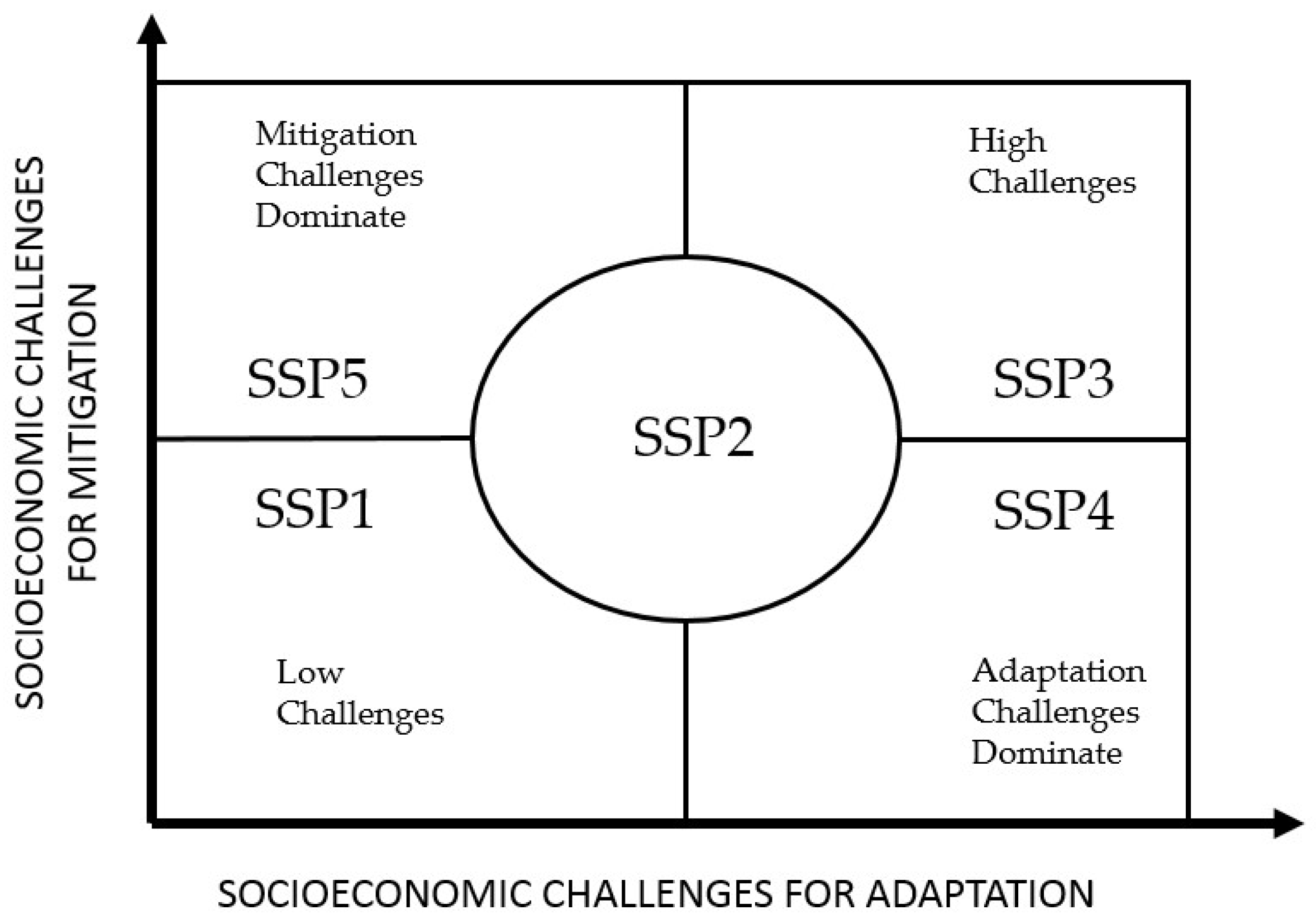
In addition to the above formulas, the projection of water risk for the cities in Iran, Iraq and Saudi Arabia with populations greater than one million from 2020 to 2030 has been completed. This analysis models potential changes in the future demand and supply of water for the selected cities with populations greater than one million. The following indicators were used: (a) estimated indicators of water demand (a1) withdrawal and (a2) consumptive use; (b) water supply; (c) water stress (the ratio of water withdrawal to supply) and (d) inter-annual (seasonal) variability for the period between 2020 and 2030. This was completed for each of the two climate scenarios, representative concentration pathways RCP, specifically RCP4.5 and RCP8.5, and two shared socioeconomic pathways, Shared Socioeconomic Pathways (SSP), SSP2 and SSP3. RCP 8.5 is a status quo scenario of relatively unconstrained emissions. Temperature increases of 2.6 to 4.8 °C by 2100 as compared to levels from 1986 to 2005. The other scenario RCP4.5 represents a relatively optimistic scenario. In RCP4.5, temperatures rise 1.1 to 2.6 °C by 2100 [26]. Shared socioeconomic pathways are depicted in Figure 1. Data of SSPs come from [22].

The primary variables that are used for SSPs are Gross Domestic Product (GDP), population, and urban expansion and development (Urbanization). Urbanization is defined as the share of the population living in urban centers. SSP2 has a lower level of population growth, higher GDP growth, and an increased rate of urbanization. These factors can impact levels of water usage. All Shared Socioeconomic Pathways are utilized on a domestic scale [22].

These variables are estimated based on general circulation models (GCMs) from the Coupled Model Inter-comparison Project Phase 5 (CMIP5) from [27]. Additionally, mixed-effects regression models based on projected socioeconomic variables from the International Institute for Applied Systems Analysis (IIASA)’s Shared Socioeconomic Pathways (SSP) database are used [3].

Next, the analysis of drought in Iran, Iraq and Saudi Arabia is completed within a regression framework using the ordinary least square method that attempts to find the best unbiased linear estimating relationship. This relationship can be written as:

$$y=x\beta +\epsilon$$

(10)

where $y$ is the dependent variable (change in the crop production index) and together with $\epsilon$ represent $n by1$ vector with the individual observational values (n) and $x$ is the dependent variable of precipitation. It has a form of a $n by p$ matrix with the values of regressors (p). The ordinary least squares (OLS) model assumes the independent and identically distributed random variables with zero mean and standard deviation squared $\left({\sigma }^2\right)$ variance. This method tries to estimate the dependent variable y which is the change in the crop production index (dimensionless) for the years 1993 to 2015 as a function of an independent variable x, which is the precipitation level (annual sum in mm) for the years 1993 to 2015.

This is done for all selected countries in the Middle East. It must be acknowledged that before the selection of the regression framework, both time series for each country were tested for the existence of a unit root with negative results. All of the time series are therefore stationary, and the regression framework can be used.

Finally, the authors decided to merge the analyzed data into the panel framework to combine cross-sectional and time-series peculiarities of the data. Our panel data contains observations of the change in the crop production index and precipitation (mm) obtained over multiple time periods for the three analyzed countries (Iran, Iraq, Saudi Arabia). We constructed a balanced panel of three cross-sectional units over the years 1993–2015.

Firstly, the selection of an appropriate estimation technique was tested for the analyzed data. Authors considered three possible techniques: (1) pooled-OLS estimation; (2) fixed-effects model; and (3) random-effects model [28]. The pooled-OLS estimation is simply an application of Equation (10) on the panel data. The fixed-effects model can be written as:

$$Y_{it}={\beta }_{i}X+{\alpha }_i+u_{it}$$

(11)

where α_i (i = 1…n) is the unknown intercept for each country (3 country-specific intercepts). Y_it is the dependent variable of the change in the crop production where i = country and t = time. X_it represents one independent variable of precipitation, β1 is the coefficient for the independent variable and u_it is the error term. The fixed-effects model controls for all time-invariant differences between the analyzed countries, so the estimated coefficients of the fixed-effects models cannot be biased because of omitted time-invariant characteristics [28].

The random-effects model differs from the fixed effects model so that the variation across entities is assumed to be random and uncorrelated with the predictor or independent variables included in the model. As it may be true that there are differences across countries that have some influence on the dependent variable, it is necessary to also test for the random-effects model. The random-effects model can be written as:

$$Y_{it}=\beta X_{it}+\alpha +u_{it}+{\epsilon }_{it}$$

(12)

where u_it is between-entity error and ${\epsilon }_{it}$ is within-entity error and all other variables are as specified above [28]. The researchers tested for the appropriate model using the F-test test, the Breusch–Pagan test and finally, the Hausman test. In their study, the authors did not consider dynamic panel data.

3. Results

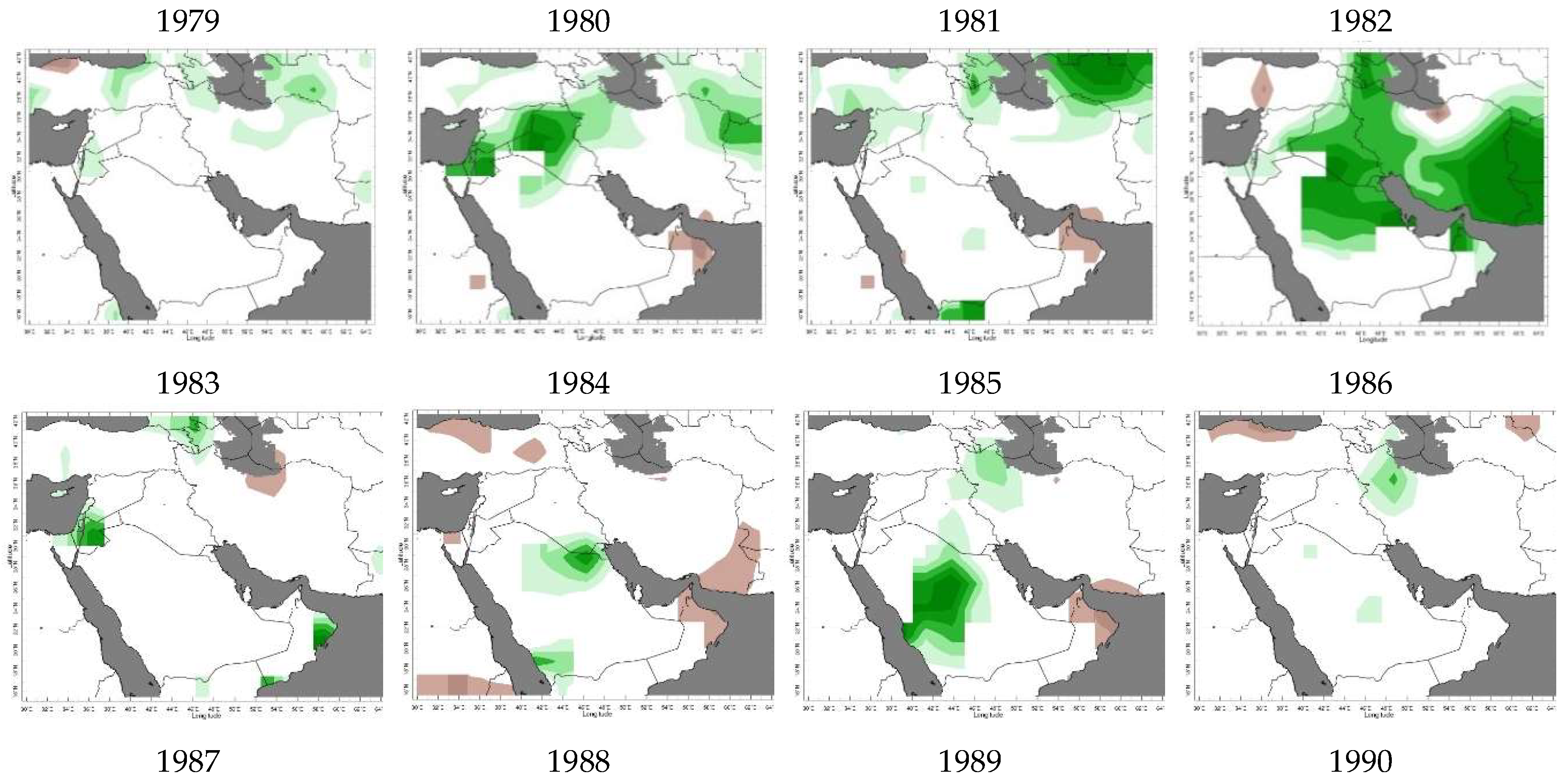
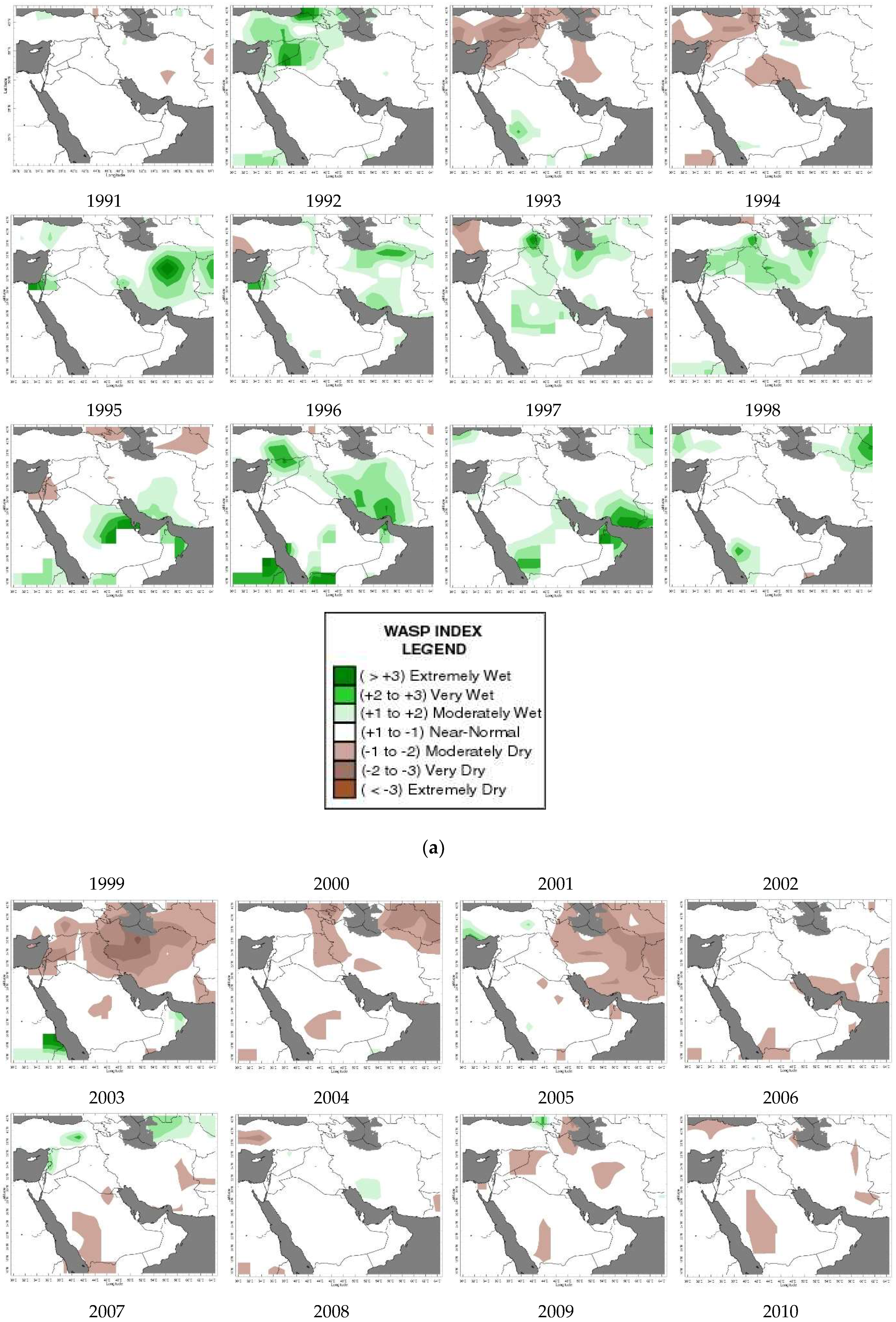
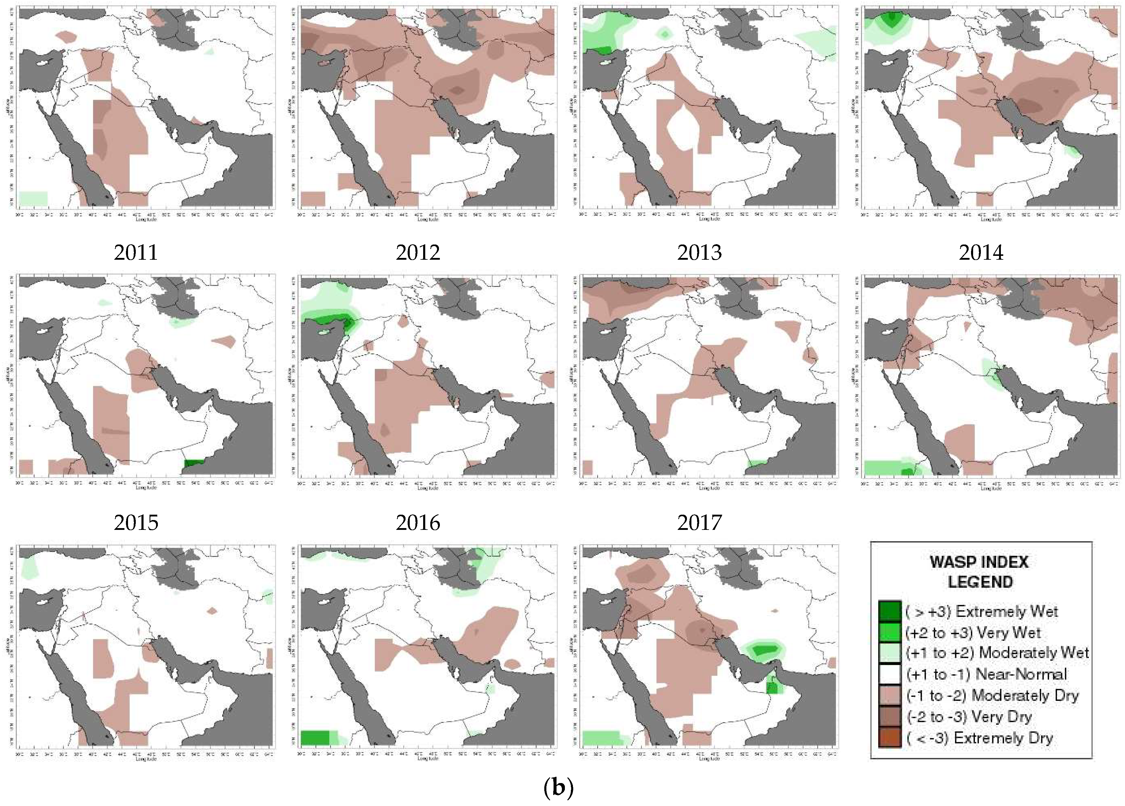
The Figure 2a,b show the “Weighted Anomaly Standardized Precipitation” (WASP) Index for the selected Middle Eastern countries from 1979 to 2017 on an annual basis. On the horizontal axis is longitude (°), and on the vertical axis is latitude (°).

For the WASP Index, shading begins at +/−1.0, with green shades indicating unusually wet conditions and brown shades indicating unusually dry conditions. Regions with an annual average precipitation of less than 0.2 mm/day are not shown on the plot. The map in Figure 2a confirms that there has not been any major drought in the analyzed countries between 1979 and 1998. While individual differences exist across both time and space, analyzed region as a whole, does not suffer from any significant droughts. Figure 2b displays the WASP index for the years from 1999 to 2017.

From Figure 2b, it is clear that in 1999, a major drought in the analyzed region occurred. This drought ushered a period of unusually dry conditions, which is still ongoing for the selected countries of the Middle East (2017). We can identify the worst years to be the years 2008, 2010 and presumably 2017.

In

Table 1. Risk for selected Middle Eastern cities with populations greater than one million.

Cities	Overall Water Risk	Physical Risk Quality	Physical Risk Quantity	Regulatory & Reputational Risk	Baseline Water Stress	Inter-Annual Variability
Saudi Arabia
Riyadh	(3–4)	(1–2)	(4–5)	(2–3)	(>80%)	4. High (0.75–1.0)
Jeddah	(3–4)	(4–5)	(4–5)	(2–3)	(>80%)	3. Medium to high (0.5–0.75)
Mecca	(3–4)	(1–2)	(4–5)	(2–3)	(>80%)	5. Extremely high (>1.0)
Medina	(3–4)	(1–2)	(4–5)	(2–3)	Arid & low water use	5. Extremely high (>1.0)
Al-Ahsa	(3–4)	(0–1)	(4–5)	(2–3)	Arid & low water use	4. High (0.75–1.0)
Ta’if	(3–4)	(0–1)	(4–5)	(2–3)	Arid & low water use	5. Extremely high (>1.0)
Iran
Tehran	(3–4)	(4–5)	(3–4)	(1–2)	(>80%)	1. Low (<0.25)
Mashhad	(3–4)	(4–5)	(4–5)	(1–2)	(>80%)	3. Medium to high (0.5–0.75)
Isfahan	(2–3)	(3–4)	(3–4)	(1–2)	(>80%)	3. Medium to high (0.5–0.75)
Karaj	(3–4)	(4–5)	(3–4)	(1–2)	(>80%)	2. Low to medium (0.25–0.5)
Tabriz	(3–4)	(3–4)	(4–5)	(1–2)	(>80%)	3. Medium to high (0.5–0.75)
Shiraz	(3–4)	(3–4)	(4–5)	(1–2)	(>80%)	5. Extremely high (>1.0)
Qom	(3–4)	(3–4)	(4–5)	(1–2)	(>80%)	3. Medium to high (0.5–0.75)
Ahvaz	(2–3)	(3–4)	(3–4)	(1–2)	(>80%)	3. Medium to high (0.5–0.75)
Iraq
Baghdad	(2–3)	(3–4)	(2–3)	(2–3)	(40–80%)	2. Low to medium (0.25–0.5)
Al Basrah	(2–3)	No Data	(2–3)	(2–3)	(10–20%)	2. Low to medium (0.25–0.5)
Al Hillah	(2–3)	(3–4)	(2–3)	(2–3)	(40–80%)	2. Low to medium (0.25–0.5)
Al Najaf	(2–3)	(3–4)	(2–3)	(2–3)	(40–80%)	2. Low to medium (0.25–0.5)
Karbala	(2–3)	(3–4)	(2–3)	(2–3)	(40–80%)	2. Low to medium (0.25–0.5)
Mosul	(2–3)	(2–3)	(1–2)	(2–3)	(20–40%)	2. Low to medium (0.25–0.5)
Erbil	(2–3)	(2–3)	(2–3)	(2–3)	(20–40%)	3. Medium to high (0.5–0.75)
Sulaymaniya	(3–4)	(4–5)	(3–4)	(2–3)	(>80%)	3. Medium to high (0.5–0.75)

The risk scale is 0–5, where 0 is no risk and 5 extreme risk.

, based on the composite index, the overall water risk identifies areas with higher exposure to water-related risks. Physical Risks Quality identifies areas of concern regarding water quality that may impact short- or long-term water availability. The model considered the following categories: (1) return flow ratio gauges the proportion of water that has been previously used and discharged upstream as waste water. Higher values mean an increased reliance on treatment plants and potentially poor water quality in locations that lack an adequate treatment infrastructure; and (2) upstream protected land shows the proportion of total water supply that comes from protected ecosystems. Lower values indicate areas located downstream from less protected watersheds. Due to this, water quality may be negatively affected in that area [23].

Regulatory Risks indicate locations of concern related to uncertainty in regulatory change, in addition to clashes with the public over water issues. This includes Access to Water which gauges the proportion of population that does not have improved drinking water sources available. Higher values highlight regions where inhabitants have limited accessibility to adequate drinking water resources, and indicate higher regulatory risks related to equal water distribution [23].

The data was collected to analyze the overall water risk for cities in the selected Middle Eastern countries with populations greater than one million. The water risk is based on a composite index with a scale from 1 to 5. The overall water risk index has been converted into values on a scale from 1 to 5, with 1 = low risk (x < 25%), 2 = medium risk (25% < x < 50%), 3 = high risk (50% < x < 75%), 4 = very high risk (75% < x < 80%) and 5 = extremely high risk (x>80%), with the mean of 3.4 and a 95% confidence interval of the mean from 3.2 to 3.6, indicating a high to extremely high risk. The results revealed a high risk (25% < x < 75%) for every city in Saudi Arabia, a majority of the cities in Iran and only one city in Iraq. Furthermore, a medium to high risk (50% < x < 80%) was found for two cities in Iran and every city in Iraq except for Sulaymaniya. In terms of Physical Risk Quality, the worst results are in Iran. In terms of Physical Risk Quantity, the worst results are found in Saudi Arabia. Regulatory and reputational risks are lowest in Iran. Extremely high baseline water stress (x > 80%) was revealed for every city in Iran, two cities in Saudi Arabia and one city in Iraq. Inter-annual Variability is generally speaking, the lowest in Iraq as opposed to Saudi Arabia and Iran.

The data collected for the projection of water risk for selected Middle Eastern cities with populations greater than one million for the period of 2020 to 2030 revealed an extremely high level of water stress (x > 80%) for all of the Iranian cities considered and most of the analyzed cities in Iraq and Saudi Arabia, with the largest projected change (2x increase in 2030) found to be in Mashhad and Tabriz in Iran and Erbil in Iraq.

Table 2. Projection of Water Risk for selected Middle Eastern cities with populations greater than one million.

Cities 2020–2030	Projected Change in Water Stress	Future Water Stress	Projected Change in Seasonal Variability	Future Seasonal Variability	Projected Change in Water Supply	Projected Change in Water Demand
Saudi Arabia
Riyadh	Near normal	(>80%)	Near normal	(<0.33)	1.2x decrease	Near normal
Jeddah	Near normal–1.4x increase	(>80%)	Near normal	(<0.33)	Near normal	1.2x increase–1.4x increase
Mecca	Near normal–1.4x increase	(>80%)	1.1x increase	(<0.33)	Near normal	1.2x increase–1.4x increase
Medina	Near normal	Arid and low water use	No Data	No Data	Near normal	Near normal
Al-Ahsa	1.4x increase	Arid and low water use	Near normal	(<0.33)	1.2x decrease	1.2x increase
Ta’if	1.4x increase	Arid and low water use	1.1x increase	(<0.33)	Near normal–1.2x increase	1.4x increase–1.7x or greater increase
Iran
Tehran	Near normal–1.4x increase	(>80%)	Near normal	(<0.33)	Near normal	1.2x increase
Mashhad	1.4x increase–2x increase	(>80%)	Near normal	(<0.33)	1.2x decrease	1.2x increase–1.4x increase
Isfahan	1.4x increase	(>80%)	Near normal	(<0.33)	1.2x decrease	1.2x increase
Karaj	1.4x increase	(>80%)	Near normal	(<0.33)	1.2x decrease	1.2x increase–1.4x increase
Tabriz	1.4x increase–2x increase	(>80%)	Near normal	(1.0–1.33)	1.2x decrease–1.4x decrease	1.2x increase–1.4x increase
Shiraz	Near normal	(>80%)	Near normal–1.1x increase	(0.66–1.0)	Near normal	Near normal
Qom	1.4x increase	(>80%)	Near normal	(0.66–1.0)	1.2x decrease	1.2x increase
Ahvaz	1.4x increase	(>80%)	Near normal	(0.66–1.0)	1.2x decrease	Near normal–1.2x increase
Iraq
Baghdad	1.4x increase	(40–80%)–(>80%)	Near normal	(1.0–1.33)	1.2x decrease	1.2x increase–1.4x increase
Al Basrah	1.4x increase–2x increase	(>80%)	Near normal	(0.66–1.0)	1.2x decrease	1.2x increase–1.4x increase
Al Hillah	1.4x increase	(>80%)	Near normal	(0.66–1.0)	1.2x decrease	Near normal
Al Najaf	1.4x increase	(>80%)	Near normal	(0.66–1.0)	1.2x decrease	Near normal
Karbala	1.4x increase	(>80%)	Near normal	(0.66–1.0)	1.2x decrease	Near normal
Mosul	1.4x increase	(20–40%)	Near normal	(1.0–1.33)	1.2x decrease	1.2x increase
Erbil	1.4x increase–2x increase	(40–80%)	Near normal	(1.0–1.33)	1.2x decrease	1.2x increase–1.4x increase
Sulaymaniya	1.4x increase	(>80%)	Near normal	(0.66–1.0)	1.2x decrease	1.2x increase–1.4x increase

represents the realistic scenario for the years 2020–2030 for all analyzed indicators.

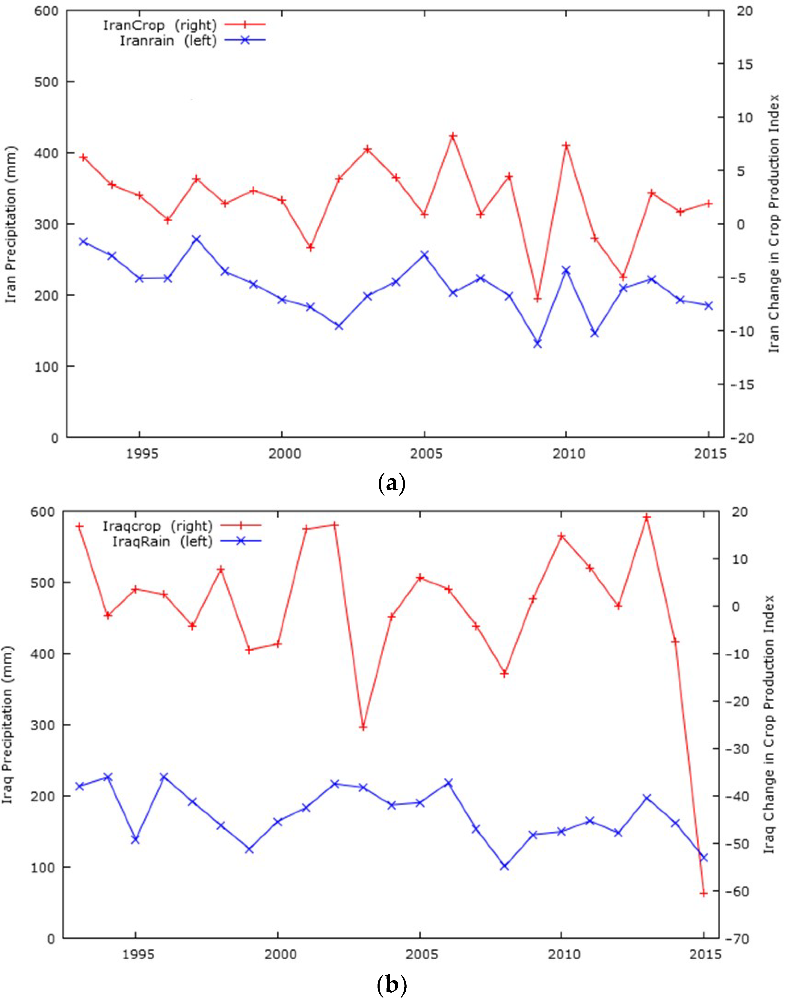
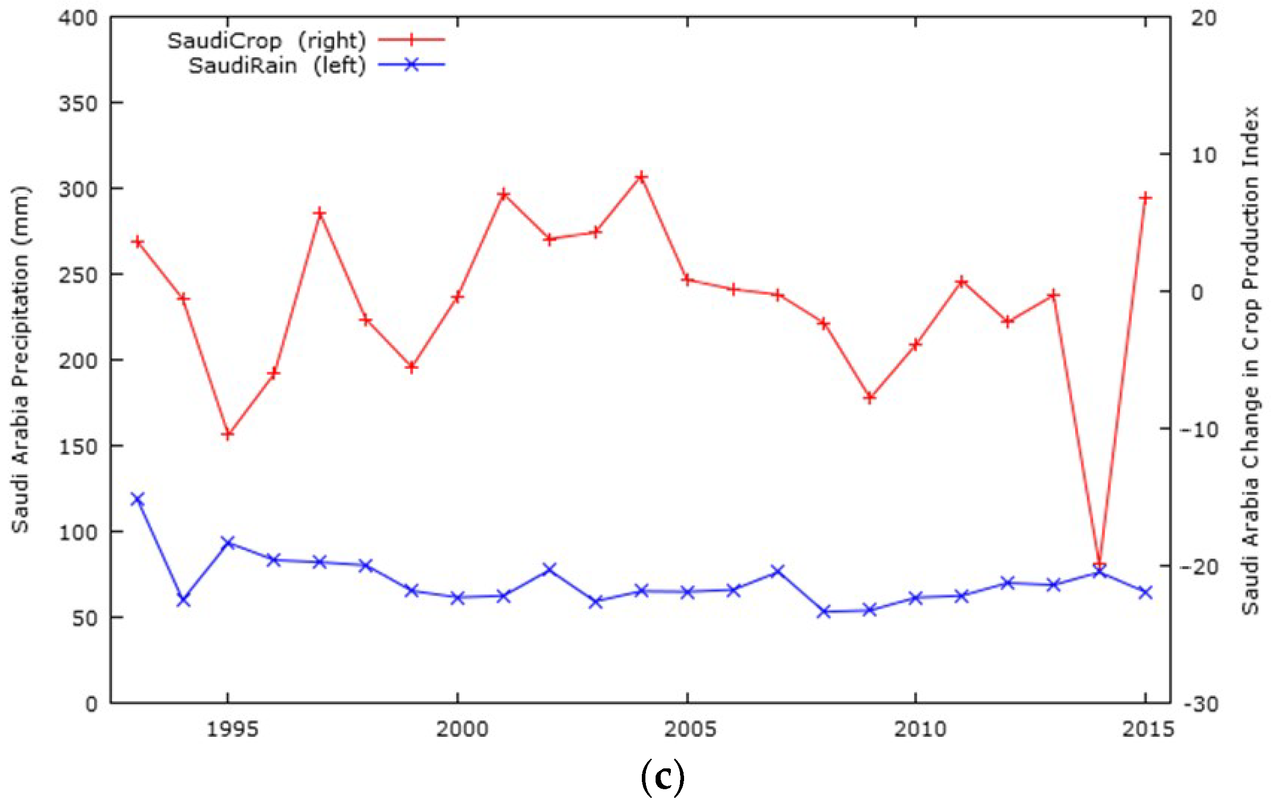
While agriculture is much more important for Iran and Iraq than it is for Saudi Arabia [12,13], it is also true for both countries that the total contribution of agriculture to the national GDP has declined. Nevertheless, it is important to analyze the impact of precipitation on agricultural output in all analyzed countries. Firstly, the precipitation data that was collected from [21] has been aggregated into annual precipitation for the years 1993 to 2015 for each country. This annual precipitation can be seen in Figure 3a–c on the left y axis. The diagrams show a slight downward trend with numerous fluctuations for all of the analyzed countries except Saudi Arabia which remains almost level. Researchers acknowledge that annual precipitation does not fully reflect peculiarities of agriculture in each of the analyzed countries, as growing seasons must be considered. In addition, it also does not consider the geographical factors of precipitation as it aggregates it into the entire region. However, it is obvious from Figure 3a that the two driest years in Iran were the years 2001 and 2008.

In Figure 3b, for Iraq, one can identify three driest years to be the years 1999 and 2008.

In Figure 3c, the driest year for Saudi Arabia is 2008.

When comparing precipitation in the Figures above, we can clearly see that while Iran has the highest level of precipitation, it also has the highest level of volatility. Additionally, data was accumulated for agricultural output in Iran, Iraq and Saudi Arabia. The authors decided to use the Crop Production Index as an indicator for agricultural output in Iran. Here, the Crop Production Index demonstrates agricultural production for each year relative to the base period of 2004 to 2006. This index encompasses all crops, in exception of fodder and fodder-related crops. Regional and income group aggregates for the FAO’s production indexes are calculated from the underlying values in international dollars, normalized to the base period of 2004 to 2006. It includes all commodities that are considered edible and contain nutrients. Coffee and tea are excluded; however, this does not constitute a large problem as they are not produced in large quantities in any of the analyzed countries. The index is based upon the sum of price-weighted quantities of various agricultural commodities produced after the deductions of quantities used as seed and feed are weighted in a similar manner. The resulting aggregate therefore represents, disposable production for any use excluding; seed and feed [18].

In this paper, the Crop Production Index for Iran, Iraq and Saudi Arabia has been transformed using first differences. The resulting change in the crop production index that is depicted in the Figure 3a–c on the right y axis demonstrates, for the most part, a positive development in the crop production in Iran, Iraq and Saudi Arabia. This, in our opinion, mainly reflects technological advancement in the industry. The graph on the left y axis demonstrates that there are three data points with the largest negative values which represent the years with the lowest aggregate precipitation.

While examining both time series in Figure 3a, it seems plausible to argue that there may be a relationship between precipitation and change in the crop production index for Iran. It seems less obvious for Iraq and Saudi Arabia in Figure 3b,c. Therefore, these relationships must be quantitatively examined using a proper methodology. As none of the time series indicate the existence of a strong trend, it was possible to examine the relationship between these time series using linear regression which produces the best unbiased linear estimator.

Results of the individual regressions are presented in

Table 3. Regression results (Iran, Iraq, Saudi Arabia) using observations 1993–2015 (n = 23).

Indicators	Coefficient	Std. Error	t-Ratio	p-Value
Iran
Constant	−7.32797	4.15078	−1.7654	0.09203
Precipitation	0.05	0.0193471	2.35	0.02885 **
Iraq
Constant	−35.4101	16.2854	−2.1743	0.04126 **
Precipitation	0.2	0.0919251	2.16	0.04233 **
Saudi Arabia
Constant	1.11	6.89064	0.16	0.87313
Precipitation	−0.0280786	0.0953258	−0.2946	0.77123
	Iran	Iraq	Saudi Arabia
R-squared	0.21	0.182026	0.004115
Durbin–Watson	2.53	1.465817	1.877329
Adjusted R-squared	0.17	0.143075	−0.043309

** significant on 90% level.

. These tables show the estimates of the relationships between the dependent and the independent variables.

The model for Iran can be written as:

$$y= -7.32797+0.04539+ ϵ$$

(13)

The results of Iranian regression show that precipitation ceteris paribus may be with a certain degree of uncertainty, one of the factors that influences crop production in Iran. It is statistically significant at a level of 90%. Furthermore, the coefficient shows that as precipitation increases by one unit (one mm), there is a positive change in the crop production index by approximately 0.05. The value of the intercept is −7.32. This indicates an influence of other factors that are omitted from the regression. In addition, the coefficient of determination is quite low. This is due to the existence of other variables that can explain changes in crop production such as, various inputs of production (land, labor, machinery, fertilizers, chemicals). Their analysis, however, is not the main goal of this paper. The Durbin–Watson statistics indicate that the residuals are serially independent.

The results of regression analysis for Iraq show that precipitation ceteris paribus could be one of the factors that influence crop production in Iraq. It is statistically significant at a level of 90%. When precipitation increases by one unit (one mm), there is a positive change in the Crop Production Index by approximately 0.19. This means that precipitation may have a much larger impact on crop production in Iraq than in Iran. The value of the intercept is −35.41. This indicates an influence of other factors that are omitted from the regression. In addition, the coefficient of determination is even lower than in Iran. This can again be explained by existence of other variables that can influence changes in crop production such as the amount of land, labor, machinery, fertilizers and chemicals. The extremely low value of R-squared makes the results of this regression doubtful. The Durbin–Watson statistics indicates that the residuals are serially independent.

According to the results of regression analysis for Saudi Arabia, we can argue that precipitation does not influence crop production in Saudi Arabia. It is statistically insignificant. This means that while crop production in Iran and Iraq may be influenced by precipitation, it is not true for Saudi Arabia. This may be due to nature of their agricultural production and slightly different agriculture related climatic conditions [11,12,13].

Finally, all of the data was put into a balanced panel with three cross-sectional units observed over 23 periods (1993–2015). Firstly, the data was estimated using OLS and then tested for the most appropriate estimation approach using panel diagnostics.

The first hypothesis for which the data was tested was the null hypothesis that the pooled OLS model is adequate, and in favor of the fixed effects alternative. The fixed effects estimator allows for differing intercepts by cross-sectional unit. F-test yields a p-value 0.0934423. It is obvious that the p-value is higher than the critical value and, therefore, the pooled OLS model seems to be more adequate against the fixed effects alternative. Next, the data was tested for the existence of random effects using the Breusch-Pagan test statistic. Breusch-Pagan test yields a p-value of 0.560138. Again, the test yields a p-value that is greater than the critical value. Hence, we can conclude that the pooled OLS model is adequate and no random effects should be considered in the model. Finally, the Hausman test statistic yields a p-value of 0.0367147. Here, we could conclude (on 90% level) that a low p-value counts against the null hypothesis that the random effects model is consistent, in favor of the fixed effects model. Since we have already concluded that the Pooled-OLS model is more appropriate, this is not of much interest. The results of the Pooled-OLS are presented in

Table 4. Pooled OLS, using 69 observations, Included 3 cross-sectional units.

Indicators	Coefficient	Std. Error	t-Ratio	p-Value
Const	−5.43701	3.11453	−1.7457	0.08545
Prec	0.0368143	0.0187655	1.9618	0.05394

Note: R-squared is 0.054323; Durbin–Watson is 1.430746; Adjusted R-squared is 0.040208.

below.

The Durbin–Watson test statistics results are relatively normal. R-squared and adjusted R-squared are very low. Due to heterogeneity, the coefficient of determination is usually not very high in panel data. Since the coefficient itself is insignificant, as the p-value of 0.05394 is greater than the critical value of 0.025, we can conclude that when we aggregate all of the data from the analyzed countries of Iran, Iraq and Saudi Arabia, there is little statistical evidence that the crop production is influenced by precipitation.

4. Discussion

Droughts in Middle East have been studied and analyzed by numerous researchers and authors [20,28,29]. For example, [29] studied rainfall and calculated drought severity at 10 stations in the eastern half of Iran for the period of 1966 to 2005. They concluded that all of the stations experienced at least one severe drought [29]. This is in accordance with our results which also show an on-set of droughts. Other authors evaluated the spatial distribution of the seasonal and annual precipitation in western Iran utilizing data from 140 stations from the period of 1965 to 2000. Their results show that the northern and southern regions of western Iran are characterized by vastly different climatic variability [30]. This is confirmed by our study using the WASP index. According to our results, the dry periods in Iran commenced around the year 1999.

The same methodological approach that is used in our study can be found in several studies from other authors [30,31,32]. For example, [32] studies droughts in Syria, particularly looking at the future climate-related risks for water systems while offering some water management strategies for reducing those risks [32]. The author claims that from 2006 to 2011, Syria experienced a long period of extreme drought that contributed to agricultural failures. This is in accordance with our study of Iran and Iraq which have a similar climate. However, in Iran and Iraq, droughts began seven years earlier than in Syria, thus contributing to possibly larger effects. The author does not attempt to quantify the negative effects of drought upon agricultural production in Syria.

Another publication that evaluates water stress was written by the authors of [33] and focused on the United States. In their study, researchers created water index stress maps to better understand water scarcity in the U.S. [32]. As opposed to our study, they also incorporate exogenous water transferred by rivers into the area.

A study of a relationship between the economy and droughts in Middle East has not been undertaken by many scholars. One example that estimates economy-wide impacts on the Iranian economy is [11]. In their study, they utilize a linear programming approach as opposed to our regression framework. The authors offer specific numbers, as according to their study, changes in the value added of all three sectors—the cropping sector, livestock, manufacturing and services sectors—amount to a $3.2 billion or 4.4% change in overall Iranian GDP [11]. They do not provide specific numbers for the cropping sector, so that their estimate cannot be compared with our results.

In the study of Salehi et al. [34], the authors argue that the water sector is a fundamental and basic part of any national economy. It is directly linked to the growth of other sectors, especially the agricultural sector and its sub-sectors. They look at the groundwater use in Iran and argue that there are unsustainable practices in use in Iran and warn about possible future water stress. This is confirmed by our study that also predicts water stress in many areas of Iran. Other authors use similar methodology to identify and forecast water risk for Iran. They only qualitatively describe that droughts in Iran will negatively influence agricultural yield, yet, with no quantification efforts. Specifically, they claim that the economic impact of water scarcity is characterized by a disproportionately high expense input to the agricultural product output or yield [35].

The agricultural sector in Iran, Iraq or Saudi Arabia has mainly been studied and written about by these authors [36,37]. According to their study, rainfall water alone is unable to support the ongoing agricultural irrigation practice. They deem agriculture as the main water withdrawal sector. They also identify the major droughts in accordance to our study [36,37]. The relationship between weather measured by hydrothermal indices and yield has been examined by several authors [38,39]. The authors use one factor for detecting the relationship between climate and crop production and discovered that inter-seasonal variability may play an important role [39]. This is in accordance with our results where we identify inter-seasonal risks for all analyzed areas to be high. However, it must be acknowledged that, generally the importance of the agriculture sector for national economies has decreased worldwide [40,41,42,43,44]. This is also true according to our review of selected Middle Eastern economies, particularly Saudi Arabia.

In terms of future climatic conditions in the region, researchers estimate that variability of weather will change with onsets of long dry periods [45,46,47]. This will lead to further economic losses. It is estimated [10] that one millimeter of rainfall creates a value of USD 14.5 million in Iran. Otherwise stated, a 1% decrease in precipitation below the long-run average results in a 0.68% decline in the value added of the agriculture and horticulture sector [10]. If we consider our results of one unit increase of rainfall increasing crop production index by 0.04, the value of $14.5 million seems to be exaggerated.

5. Conclusions

Climate change is most certainly a global issue, but it also has dire domestic consequences that are often overlooked. When coupled with the already arid geographic location of the Middle East, climate change is drastically affecting the social and economic landscape of Iran. This is obvious from our graphical maps constructed using WASP, which show drier conditions beginning in 1998 for all analyzed countries.

With this in mind, it is apparent that expert scientific management is crucial to resolving the current water crisis in the region. According to our research, analyzed Middle Eastern cities are experiencing and will continue to experience a high overall water risk, with extremely high baseline water stress. This is apparent from the results that show that 20 out of 22 analyzed cities may experience future water stress (2020–2030). This means that each of the analyzed countries will probably experience water stress in the future. Still, some differences among the analyzed countries were found. Based on our results, Iran may experience the worst degradation of this water-related situation.

In this study, the authors found weak evidence of a negative relationship between precipitation in Iran and crop production. Specifically, our results indicate that as precipitation increases by one unit (one mm), there is a positive change in the Crop Production Index by approximately 0.04. Even though the results for Iraq are statistically less significant, it can be suggested for both countries, to immediately proceed with sustainable water saving agricultural practices. For Saudi Arabia, it is apparent that agriculture already relies heavily on irrigation and is generally less dependent upon precipitation. When we combine each of the countries into a single panel, we did not find any strong statistical evidence for the existence of a relationship between precipitation and agricultural crop production change.

Our results suggest that water demand will rise in most of the analyzed regions of Iran, Iraq and Saudi Arabia. Specifically, in 16 of the analyzed 22 regions, water demand will most definitely rise. Therefore, it is crucial to properly employ sustainable water conservation and management practices.