Relationships Among Animal Communities, Lentic Habitats, and Channel Characteristics for Ecological Sediment Management

Abstract

This study used a multiscale analysis of relationships among the bitterling and mussel communities, lentic habitat structures with conditions and flooding frequency, and channel characteristics for application in ecological sediment management. From the Kizu River in Japan, 120 lentic habitats were sampled in 2007 and 2010. The floodplain vertical shape index (FVSI), which indicates the degree of convexity or concavity of the vertical shape of a floodplain, was used as channel characteristics using historical cross-section profiles obtained from 1960 to 2012. For examining the relationships between bitterlings/mussels and each habitat condition or structure, abundance values of bitterlings and mussels were transformed into habitat suitability index (HSI). Furthermore, the relationships between the number of habitat structures and FVSI were analyzed. The results indicated that bitterlings and mussels are more abundant in terrace ponds than in active ponds, especially so in terrace ponds located in the lower area of bars with a flooding frequency of 8–16 days/year (bitterlings), those located in the lower area of bars with a flooding frequency of 8 days/year, and those located in the upper area of bars with a flooding frequency of 16–22 days/year (mussels). These ponds tended to have less than 1 cm mud depth that was negatively related to abundance of mussels. These suitable habitat types tended to be located in channels with a floodplain vertical shape index between −0.35 and 0.05. We established countermeasures to prevent channel types with floodplain vertical shape index exceeding 0.05 instead of restoring the previous channel conditions.

1. Introduction

The interruption of the natural flow and sediment transfer by dams causes changes in the flow, river structure, and ecosystem in the reservoirs and regions downstream of the dam. When reservoirs are filled with sediments, their storage capacity is reduced, affecting the water supply and hydroelectric power [1]. Downstream of dams, the reduced sediment supply results in degradation of the stability of channel structure, and the quality of aquatic habitats [2]. In order to remove sediments accumulated in reservoirs and to transport sediment downstream, several sediment management strategies such as replenishment, sluicing, and bypassing have been tested worldwide [3,4,5]. Actually, artificial sediment supplies downstream have contributed to enhancing the available spawning habitat for chinook salmon [2] and the lotic habitat quality for invertebrates and fishes [6]. In order to predict the geomorphic and environmental impacts of sediment management and for successful ecological restoration, it is essential to understand river characteristics and conditions under natural and artificial disturbances. The reach-scale channel configuration, such as braided, wandering, and straight channel, can be helpful for linkage between hydraulic conditions and aquatic ecosystems. This can be examined using hydraulic and geomorphic parameters, including discharge and slope [7], sediment load and lateral stability [8], and slope and bed materials [9]. The variations in channel configuration are in response to the flow regime and sediment transport, which further influence the geomorphic units such as ponds, bars, wetlands, backwaters, and pool-riffle sequences. Further, the assemblages of geomorphic units at the reach-scale are related to the habitat diversity and animal communities [10]. The high complexity of landforms generally equates to the high diversity of hydraulics and thus the high biodiversity [11,12]. If research related to the relationship between the channel configuration and ecosystem are efficiently conducted, it is possible to predict the impact of natural or artificial disturbances on the ecosystem [13]. Therefore, integration of ecological and geomorphological perspectives with the acknowledges the multiscale abiotic and biotic structures of a stream system is required, but is an unresolved challenge [14]. Wyrick and Rasternack [12] systematically studied the relationship between geomorphic units, hydraulic parameters, and their relevance for various habitats. Other previous studies on multiscale relationships between abiotic and biotic structures have focused on lotic habitat conditions; the relationships between lotic habitat conditions and channel configurations [15,16], landscape diversity with channel characteristics [17], or habitat diversity in specific channel types [18,19].

This study focused on multiscale relationships among animal communities, lentic habitats, and channel characteristics in the Kizu River. The Kizu River provides suitable lentic habitats such as ponds or backwaters for bitterlings and mussels on its floodplain [20]. However, the diversities of bitterlings and mussels decreased, and the protected bitterling Acheilognathus longipinnis disappeared. Therefore, the target animal communities of this study are considered to be bitterlings and mussels. Further, because bitterlings and mussels live only in lentic habitats, lentic habitat structures and conditions was considered as habitat scale. In the case of lentic habitat on floodplains, the environmental conditions are characterized by hydrological connectivity with the main river channels [21]. Flooding provides hydrological connectivity with the exchange of nutrients, sediments and organisms. Therefore, we considered not only structures but also the flooding frequency. First, this study investigates the relationships between the abundance of bitterling/mussel and lentic habitat structures/conditions with the flooding frequency. Second, the relationships between habitat structures and the reach-scale channel characteristics were investigated. The floodplain vertical shape index (FVSI) was used as the reach-scale channel characteristic. As the channel types are not numerical values, FVSI was developed in Reference [22] and represented the concave and convex floodplain shapes. Additionally, the historical changes of FVSI were calculated using the historic cross-section data. Finally, we discussed previous environmental conditions and the application of these characteristics to ecological sediment management.

2. Materials and Methods

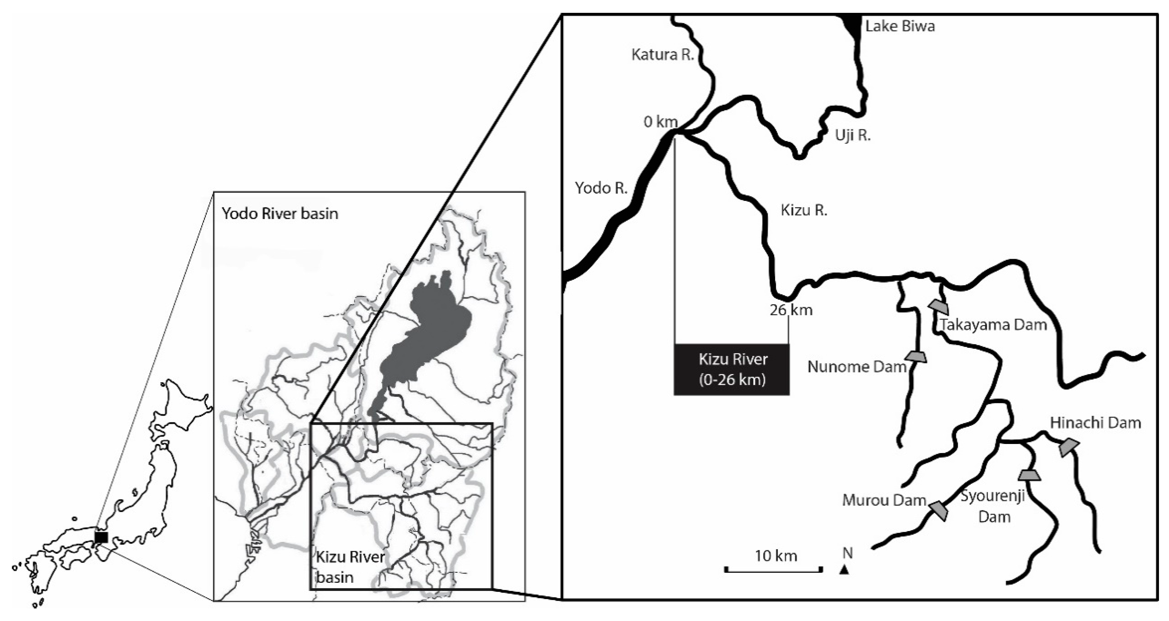
2.1. Study Site

The study area was comprised of the lower reaches (0–26 km) of the Kizu River in Japan (Figure 1). The riverbed of the Kizu River degraded, and the vegetation in the floodplain expanded after dam construction over a 65-year period. A total of five dams, namely, Takayama Dam, Syourenji Dam, Murou Dam, Nunome Dam, and Hinachi Dam, which were constructed in 1969, 1970, 1974, 1992, and 1999, respectively, are located in the Kizu River basin. The approximately 6000 m³/s peak floods occurred before the construction of dams; however, the peak of floods decreased to approximately 3000 m³/s after construction [23]. The estimated amount of bed-load transportation downstream of the dam was approximately 183,000 m³/y in the 1960s; further, it decreased to 23,000 m³/y in the 2000s (Figure 2) [13]. The reduction in the peak discharge and sediment supply upon dam construction influenced the alternation of channels from braided to single or alternating channels. These river channel changes caused the degradation of lentic habitat conditions on the floodplain owing to the reduction of inundation [20].

2.2. Data Acquisition of Bitterling and Mussel Communities

In the case of the Kizu River, because bitterlings and mussels live only in lentic habitats such as ponds and backwaters, the habitat types of pond and backwater were selected for sampling (Figure 3d,e). Prior to conducting the field survey, the size and location of the habitat were identified using aerial photos. In 2006, 190 ponds were detected in aerial photos, whereas 178 ponds were detected in 2010. Among the detected ponds, bitterlings and mussels were sampled in 47 ponds among the 190 ponds in 2007 and in 73 among the 178 ponds in 2010 by the Yodogawa River Bureau. The sampling was conducted in the summer season. Bitterlings were observed in 63 ponds and mussels were observed in 47 ponds among 120 ponds. There are five taxa of bitterlings (Acheilognathus rhombeus, Acheilognathus tabira tabira, Acheilognathus cyanostigma, Rhodeus ocellatus ocellatus, Tanakia lanceolate) and five taxa of mussels (Anodonta calipygos Kobelt, Anodonta woodiana, Lanceolaria grayana cuspidate, Lanceolaria oxyrhyncha (Martens), Unio douglasiae nipponensis) in sampling ponds. The total number (population) of bitterlings and mussels were divided by the surveyed time (h) and number of people who participated in the sampling (n), and this value was used as the abundance of bitterlings and mussels. The abundance value was used to calculate the best model of lentic habitat conditions for bitterlings and mussels. For examining the relationships between bitterlings/mussels and each habitat condition or structure, abundance values transformed into habitat suitability index (HSI) [19,20,21]. Habitat suitability index was derived by Equation (1).

$$w_i=\frac{u_i/{{\displaystyle \sum }}_{i=1}^n{u}_i}{a_i/{{\displaystyle \sum }}_{i=1}^n{a}_i}$$

(1)

$w_i$ is the ratio for the ith of n habitat categories, $u_i$ is the total abundance in category I, $\sum u_i$ is the total abundance for all habitat categories, $a_i$ is the number of samples from categories i, and $\sum a_i$ is the total number of samples [24]. The indices range from 0 to 1 for each variable, with 0 indicating the least suitable habitat conditions and 1 indicating the optimum habitat condition [25].

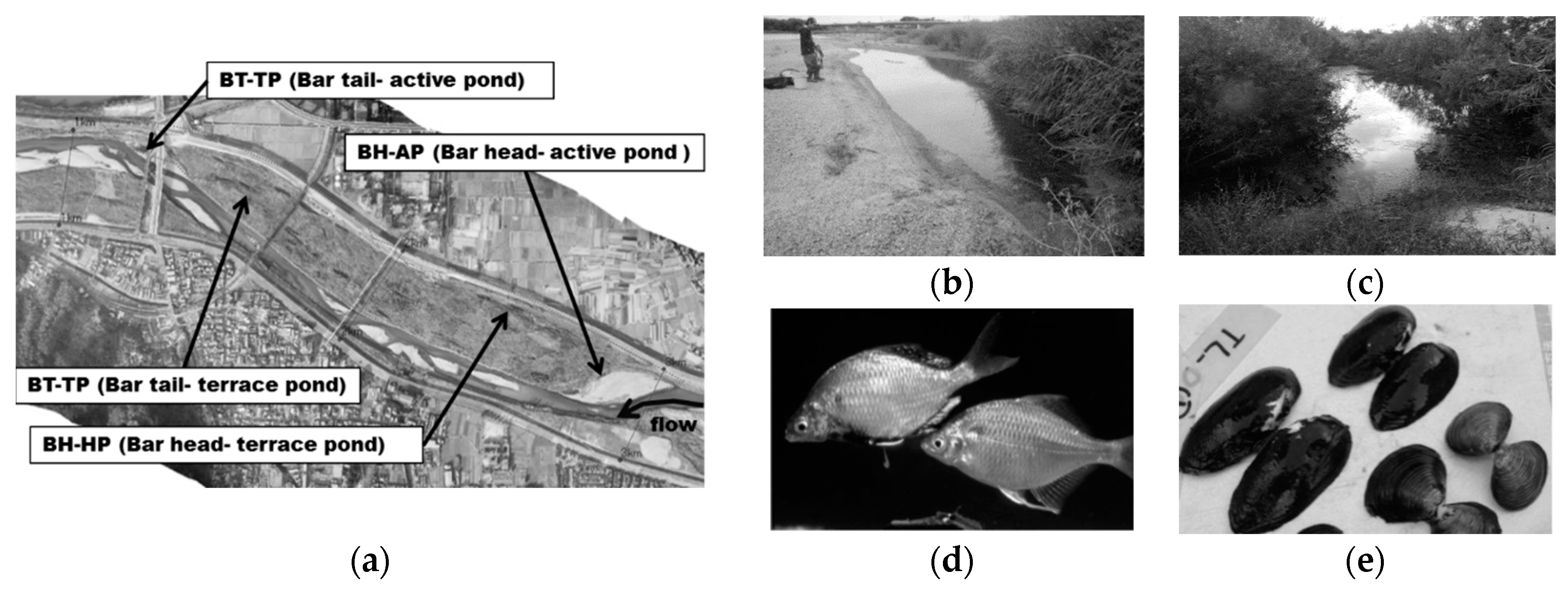
2.3. Data Acquisition of Lentic Habitat Structure and Conditions

Lentic habitat structures were classified into two types, active pond (AP) and terrace pond (TP), depending on their locations. The aerial photos obtained in 2006 and 2010 were used for this classification. AP is defined as a pond and backwater that is located on active channels such as sand-bars or sanded islands (Figure 3b), and TP is defined as a pond located on a terrace with vegetation (Figure 3c). These ponds were further classified based on the location of upper and lower sites on a particular bar. The bar was divided into two halves based on the direction of stream flow. The ponds located in the upper area were defined as bar head-ponds, whereas those located in the lower area were defined as bar tail-ponds. This classification was based on the assumption that even if the same habitat structure type was located on the same bar, the habitat conditions or the abundance of species differed depending on whether the habitats were located on the upper or lower part of the bar. Thus, four types of lentic habitats were considered: Bar head-active pond (BH-AP), bar head-terrace pond (BH-TP), bar tail-active pond (BT-AP), and bar tail-terrace pond (BT-TP) (Figure 3). A total of 190 ponds were detected in aerial photos in 2006, whereas 178 ponds were detected in 2010. Although only a total of 120 ponds were surveyed, all the detected ponds in aerial photos (n = 368) had values of the geomorphic parameters of flooding frequency. The term flooding frequency refers to the inundation frequency in a pond per year. The water level data obtained during the period from 1989 to 2008 were converted into discharge using the HQ formula. Using the converted discharge, 1 day discharge (909.1 m³, at Inooka observatory station), 8 day discharge (249.5 m³), 16 day discharge (149.0 m³), 22 day discharge (118.3 m³), 45 day discharges (72.9 m³), 71 day discharge (52.9 m³), 185 day discharge (26.2 m³) and 365 day discharge were calculated. The water level of the cross section (200 m intervals) according to each discharge was calculated using HEC-RAS software. Further, the values of water levels were overlapped with the digital elevation model (DEM) data using Geomedia 6.1 software. Thus, if the pond would be inundated based on the 1 day discharge, the pond would have a flooding frequency of 1 day/year. If the pond would be inundated based on the 8 day discharge, the pond would have a flooding frequency of 8 days/year. Therefore, the ponds have one of the following flooding frequencies: 1 day, 8 days, 16 days, 22 days, 45 days, 71 days, 185 days, and 365 days per year [26,27,28]. In this study, the flooding frequency parameter was used as the representative environmental parameter because flooding frequency is an important external condition that determines the internal habitat conditions [21]. This is especially true for lentic habitats such as wetlands or ponds. We classified the structure of the habitats by reflecting the visible geomorphic characteristics and location of the habitat to find visible targets. However, in order to compensate for the limitations of types of habitat structure identified only from aerial photos, the values of flood frequency obtained by numerical simulation were used.

In all, 7 habitat condition parameters were surveyed in 120 ponds. The parameters were as follows: Area, water depth, mud depth, mean grain size (D50), dissolved oxygen (DO), chlorophyll, and wood coverage. The previous studies examined the relationships between mussel and habitat conditions; velocity, substrate size and compaction, water depth [29]; sediment softness, velocity and sediment types [30]; water temperature and quality with the flood pulse frequency [21]. As these studies considered hydraulic habitat conditions and water quality, we determined the habitat shape (area, water depth), the substrate of habitat (mud depth and D50), and the water quality (DO and chlorophyll) to a considerable extent. The method of the survey parameters can be referenced to in the reports of References [26,27,28]. The wood coverage indicates the shaded shoreline ratio by wood, i.e., 100% wood coverage indicates that the shoreline of the pond was entirely occupied by vegetation such as that depicted in Figure 3c.

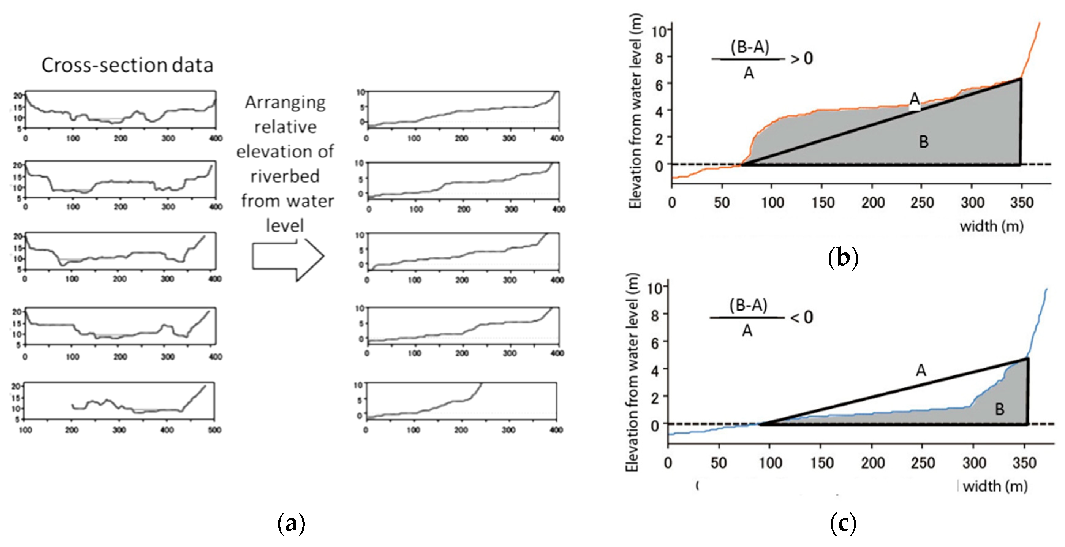
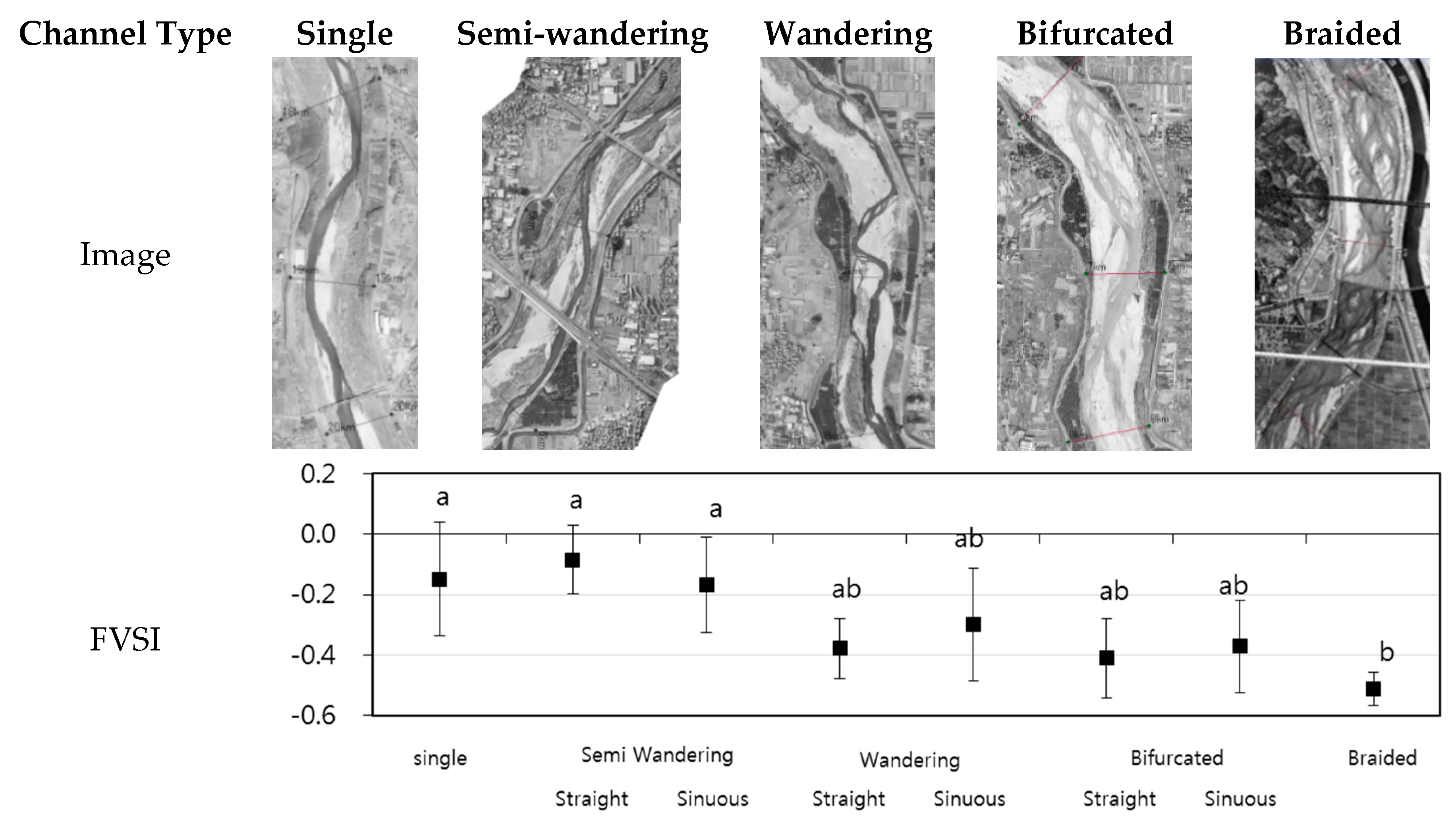
2.4. Reach-Scale Channel Characteristics

The reach-scale channel configuration in the Kizu River is categorized into single, semi-wandering-straight and sinuous, wandering-straight and sinuous, bifurcated-straight and sinuous, and braided sinuous using parameters of number of channels and sinuosity per 2 km [13]. Aerial photos obtained between 1948 and 2010 were used for performing this classification. The channel configuration of the Kizu River changed from braided channel (characterized by multi-channels and braided sand bars) to single or slightly wandering channel (characterized by less channels and wide vegetation area on the floodplain) between 1948 and 2010. However, because the channel types are not numerical values, we used floodplain vertical shape index (FVSI). This index indicates the degree of convexity or concavity of the vertical shape of a floodplain [22]. The FVSI value was calculated using cross-section data of 200 m intervals. The relative elevation of the riverbed from the water level was arranged in an ascending order. Further, we determined the area between the arranged shape (B) and the triangle connecting the following three points (A): The riverbed tangent to the water surface, bottom of the bank, and top elevation of the bank (Figure 4). The value is positive if B−A is greater than A, and negative if it is less than A. As one channel type of 2 km has 10 cross sections, 10 values are averaged in 2 km. A positive value means a convex floodplain vertical shape (Figure 4a), and a negative value indicates a concave vertical shape (Figure 4b).

The FVSI was calculated using cross-sectional data obtained between 1960 and 2010, as done in the classification of the reach-scale channel configuration in [13]. The classified reach-scale channel configurations were single, semi-wandering, wandering, bifurcated, braided channels in the Kizu River. Figure 5 depicts the average the FVSI values of the classified channel types by Tukey’s tests. The majority of the channel configurations in the Kizu River exhibited a concave floodplain vertical shape with negative values of FVSI. Although a significant difference of FVSI was not observed between single/semi-wandering and wandering/bifurcated, and the difference of wandering/bifurcated and braided, we could identify the difference between single/semi-wandering and braided channels. The single and slightly wandering channels in the Kizu River tended to have slightly convex floodplain vertical shape (−0.3 < values < 0.1), and wandering and bifurcated channels tended to have FVSI values between −0.5 and −0.1. Braided channels have a significantly concave floodplain vertical shape (values < −0.6) (Figure 5).

2.5. Statistical Analyses

In order to understand the relationships among species, habitat structures and conditions, and channel characteristics, we considered the following items in the analysis:

• A multiple regression model using the parameters of habitat conditions for the abundance of bitterlings and mussels
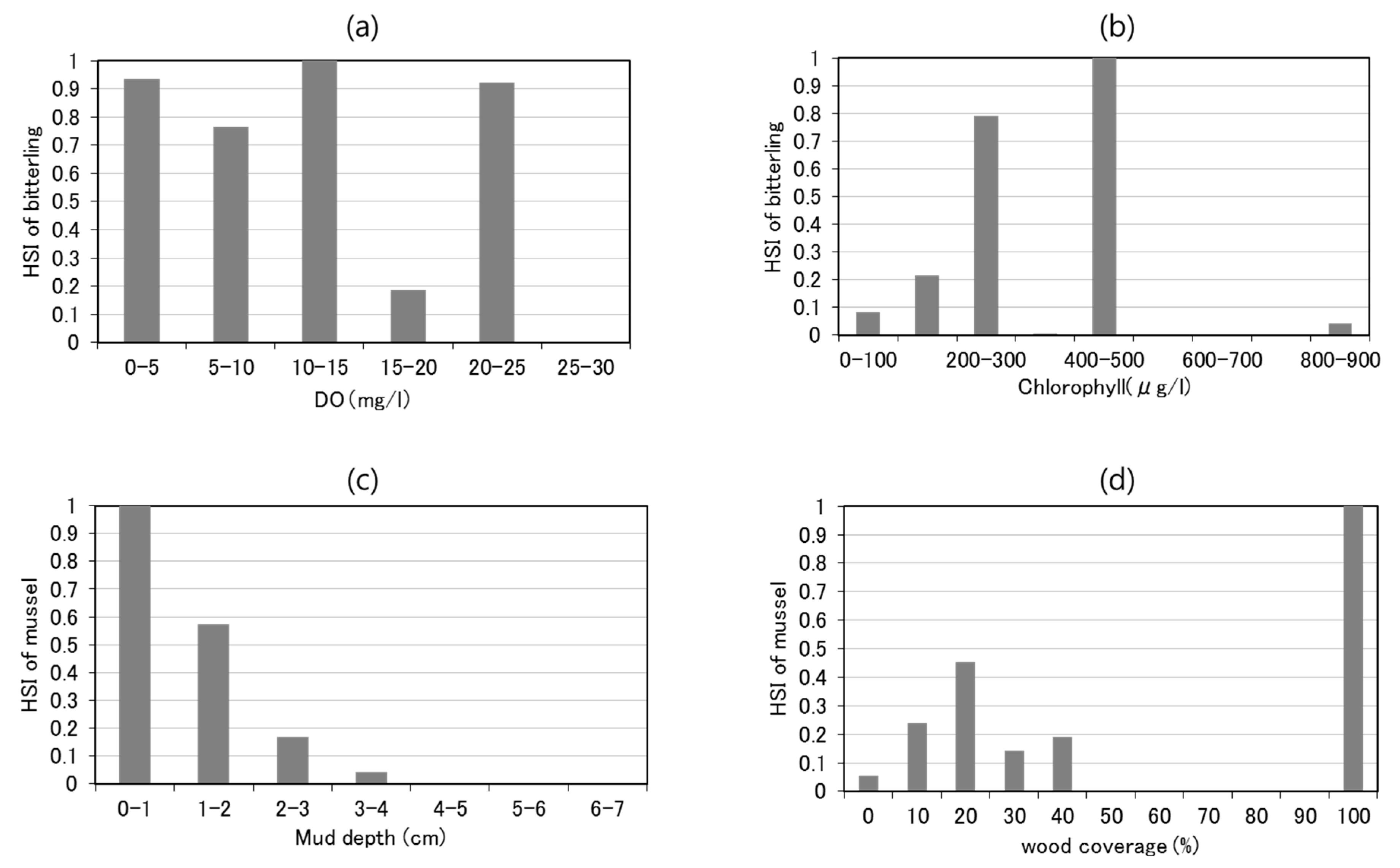
• Comparison of the habitat suitability index (HSI) of bitterlings/mussels and habitat conditions
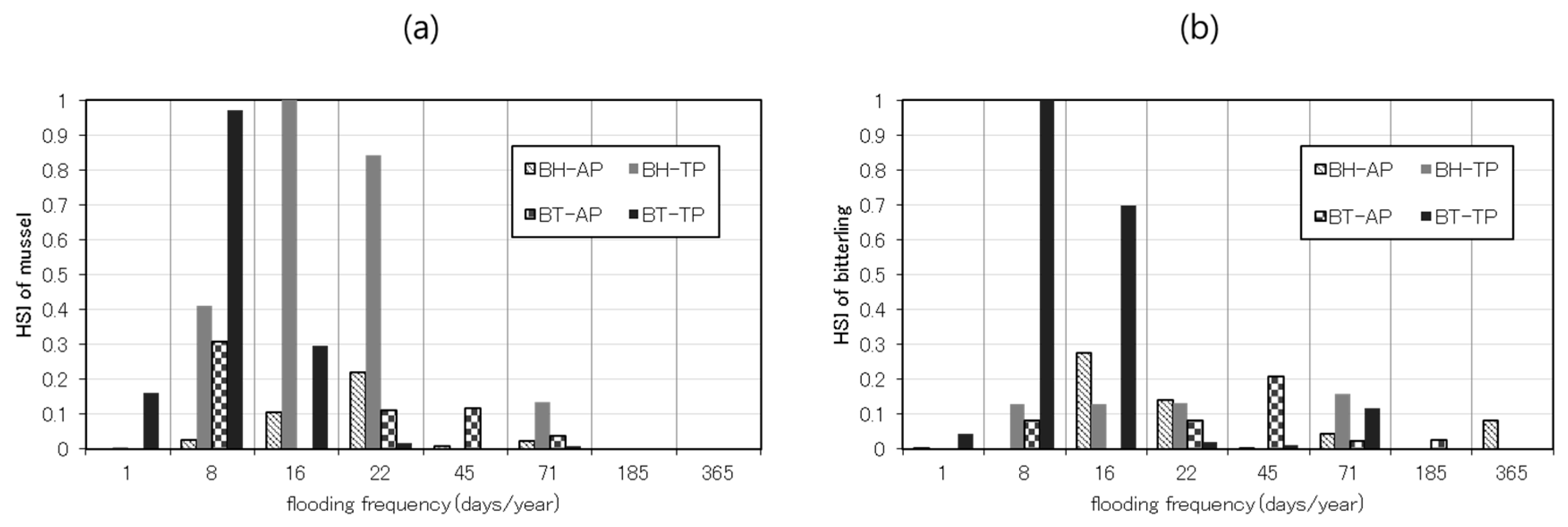
• Comparison of the HSI of bitterlings/mussels and habitat structures
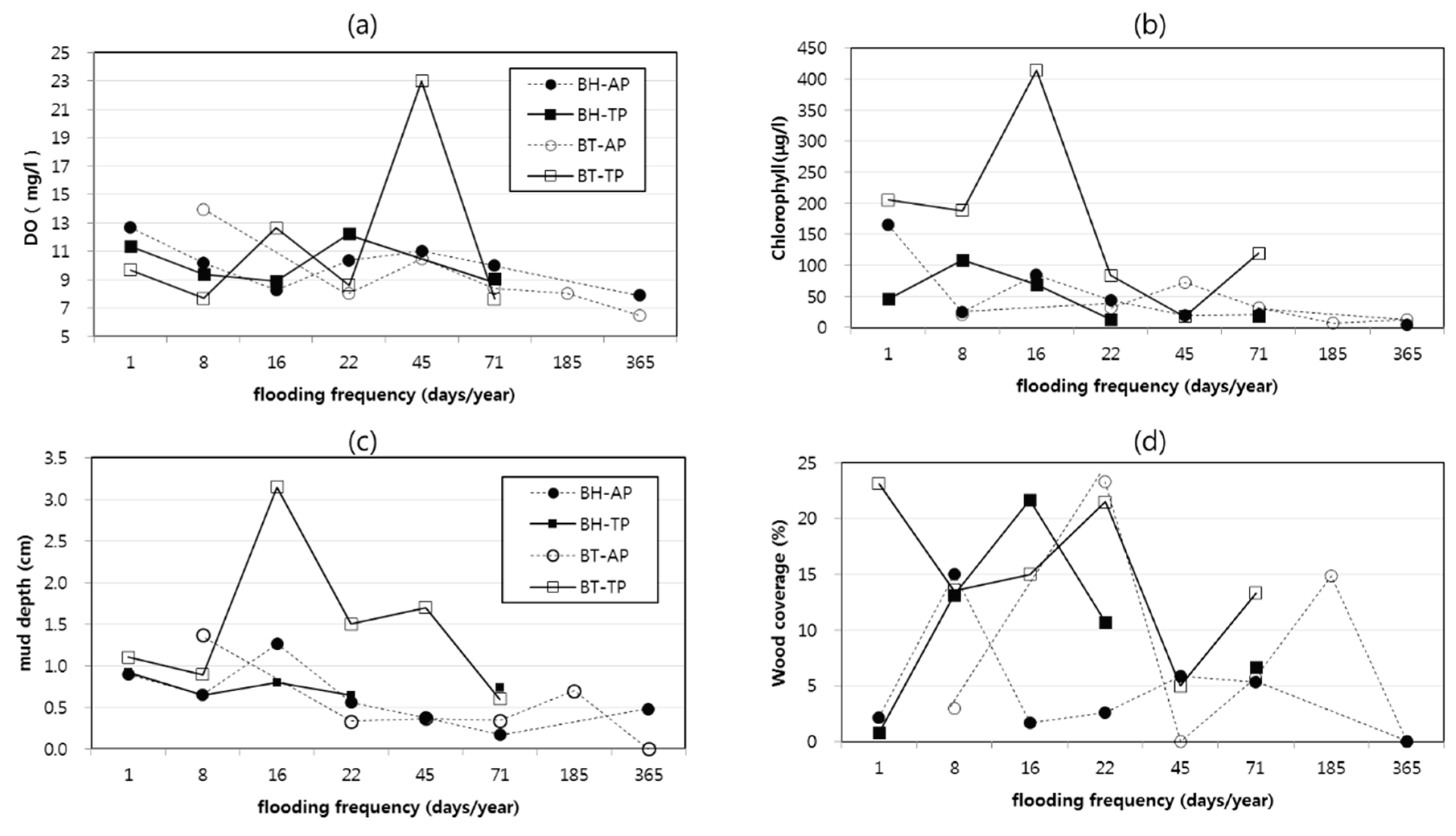
• Comparison of habitat structures and habitat conditions
• Comparison of habitat structures and FVSI

We generated multiple linear regression models with a stepwise selection method to examine the effect of habitat conditions on the abundance of bitterlings/mussels. The best model was selected based on the correlation coefficient and significance. An α value of 0.05 indicates statistical significance in the test. Further, only the parameters of habitat conditions that are related to the best models are compared with the HSI of bitterlings/mussels. Additionally, the relationship between the HSI of bitterlings/mussels and habitat conditions were analyzed. Furthermore, the relationships between habitat structures and habitat conditions were analyzed. An HSI exceeding 0.7 indicates excellent suitability. After analyzing the relationships between bitterlings/mussels and habitat structures/conditions, the relationships between the number of habitats and FVSI values were examined.

3. Results

3.1. Relationships among the Bitterlings/Mussels, Habitat Structures, and Habitat Conditions

In order to understand the relationships between the abundance of bitterlings/mussels and habitat conditions, the best models were selected based on surveyed ponds (n = 120) by using a multiple regression model. The multiple regression models were generated to test the influences of habitat conditions (area, water depth, D50, DO, Chlorophyll and wood coverage) on abundance of bitterlings and mussels. Only the parameters of habitat conditions related to the best models are listed in

Table 1. Multiple regression analysis to examine the best models of habitat conditions for the abundance of bitterlings and mussels.

Abundance	Area (cm2)	Water Depth (cm)	Mud Depth (cm)	D50 (mm)	DO (mg/L)	Chlorophyll (μg/L)	Wood Coverage (%)	Best Model
								R	p
Bitterling					−1.08 *	2.52 *		0.238	<0.05
Mussel			−1.29				2.67 **	0.272	<0.05

The best models were selected on the basis of the correlation coefficient (R) and significance (p). Values of independent variables indicate the regression coefficient (t). Significance: * p < 0.05, ** p < 0.01, *** p < 0.001.

. The abundance of bitterlings was best described by a model consisting of DO and chlorophyll (correlation coefficient: 0.238, p < 0.05), and that of mussels was best described by a model consisting of mud depth and wood coverage (correlation coefficient: 0.272, p < 0.05). Abundance of bitterlings tended to have a negative relationship with DO (regression coefficient of −1.08), whereas it tended to have positive relationships with chlorophyll (regression coefficient of 2.52). Abundance of mussels tended to have a negative relationship with mud depth (regression coefficient of −1.29) and a positive relationship with wood coverage (regression coefficient of 2.67).

The HSI values of bitterlings and mussels with the habitat conditions that are selected in the best model are shown in Figure 6. If there are no sampling points in the class or no detection of bitterlings or mussels, the result will exhibit a zero value. Although the HSI values of bitterlings decreased in 15–20 mg/L DO, this exhibited a high habitat suitability in DO case of more than 25 mg/L DO (Figure 6a). The HSI values of bitterlings tended to increase in chlorophyll between 0 and 500 μg/L and then significantly decreased after 500 μg/L (Figure 6b). The HSI of mussels exhibited the maximum score in mud depth of 0–1 cm (Figure 6c). The HSI values of mussels showed excellent suitability in 100% wood coverage (Figure 6d). There was no sampling pond with wood coverage of 60% and 80%, and number of mussels in ponds with wood coverage of 50, 70 and 90% was very low. Therefore, HSI of mussels showed about zero values in these groups.

The HSI values of bitterlings and mussels are explained by considering the habitat structures with the flooding frequency observed for 120 ponds (Figure 7). Among terrace ponds, BT-TP with a flooding frequency between 8 and 16 days/year showed excellent suitability for bitterlings (Figure 7a). BT-TP and BH-TP with flooding frequencies of 8 days/year and 16–22 days/year exhibited excellent suitability for mussels, respectively (Figure 7b). That is, the terrace ponds (BH-TP and BT-TP) with a flooding frequency between 8 and 22 days/year tended to have high HSI values for bitterlings and mussels.

Figure 8 illustrates the relationships between habitat environmental conditions and habitat structures with flooding frequency. Almost all the habitat structures, except those with a flooding frequency of 45 days of BT-TP, exhibited an average of between 7 and 13 mg/L of DO (Figure 8a). Values of chlorophyll in BT-TP with flooding frequency of 1, 8, 16, and 22 days were higher than other habitat types in the same flooding frequency (Figure 8b), and the values of mud depth in BT-TP with flooding frequencies of 16, 22, and 45 days were highest as compared to other habitat structures (Figure 8c). Further, the relationship between wood coverage and habitat structures with flooding frequency could not detect obvious difference (Figure 8d).

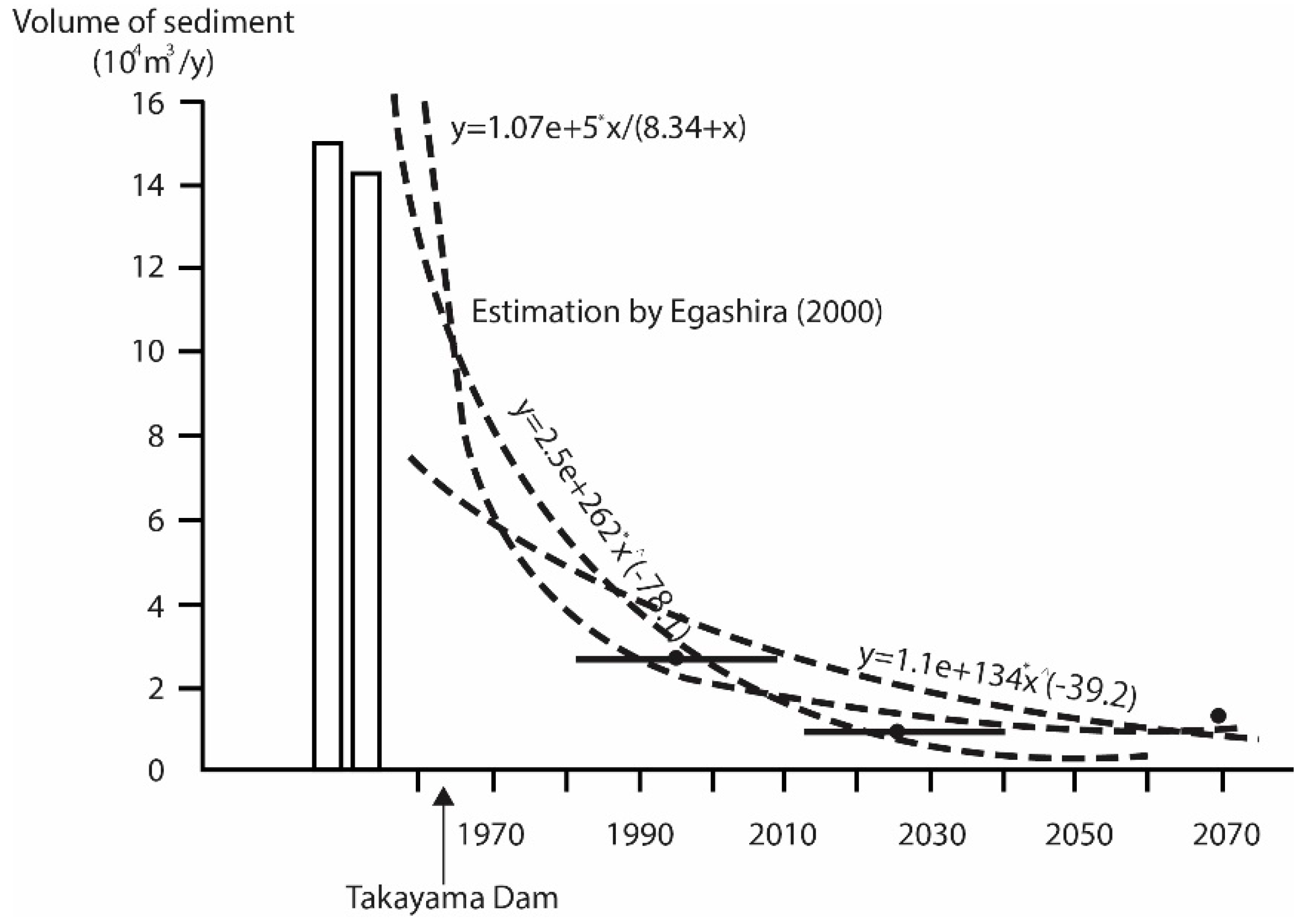
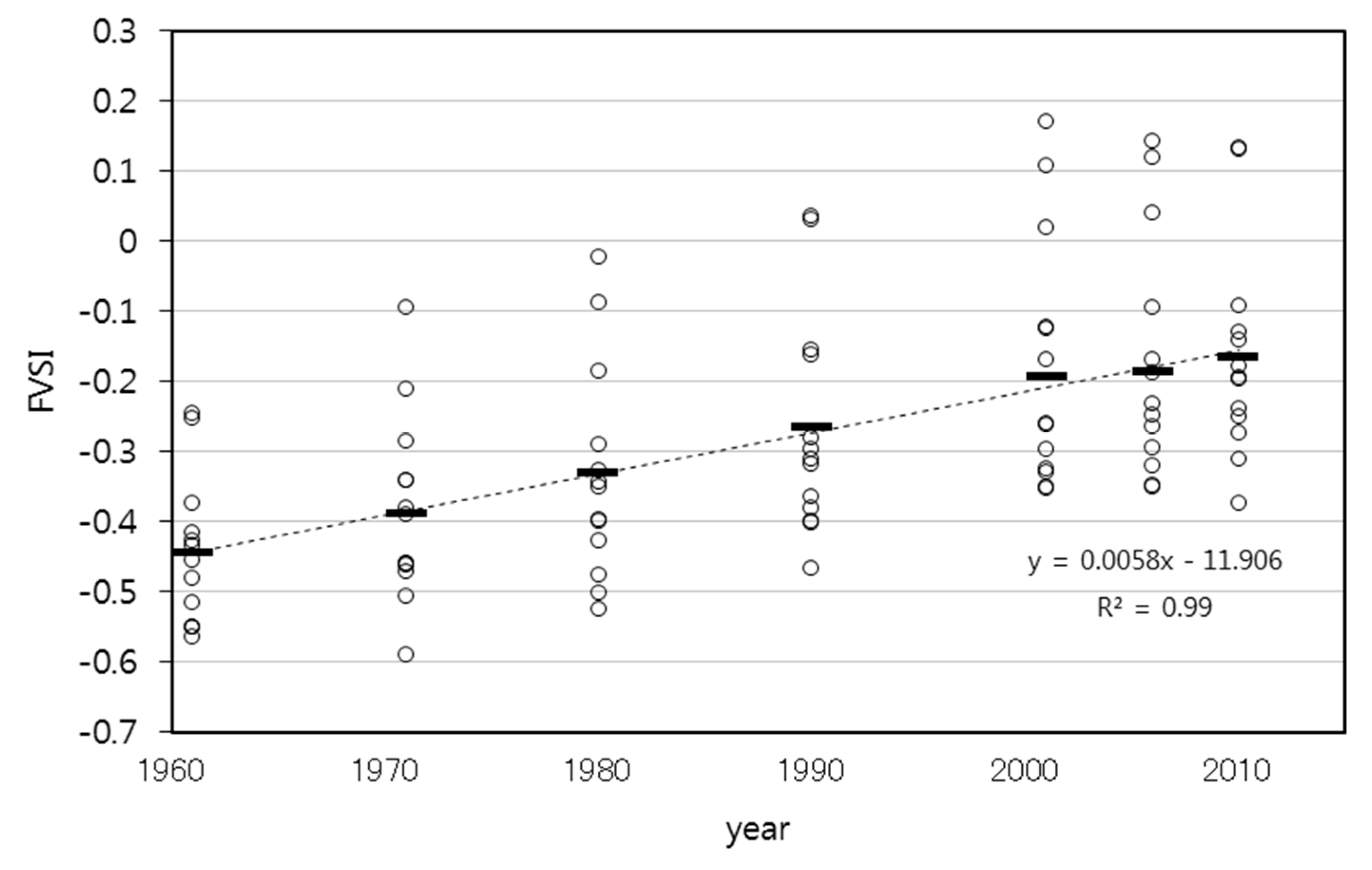
3.2. Historical Changes in FVSI

The values of FVSI per year were shown in Figure 9. As the study area extends to a length of 26 km, 12 FVSI values were obtained per year. Average FVSI increased from −0.44 in 1960 to −0.17 in 2010. The cross-sectional floodplain shape of the Kizu River tended to show convex shapes during the 60 years. Since 1990, only values of one or two sections had an FVSI > 0.

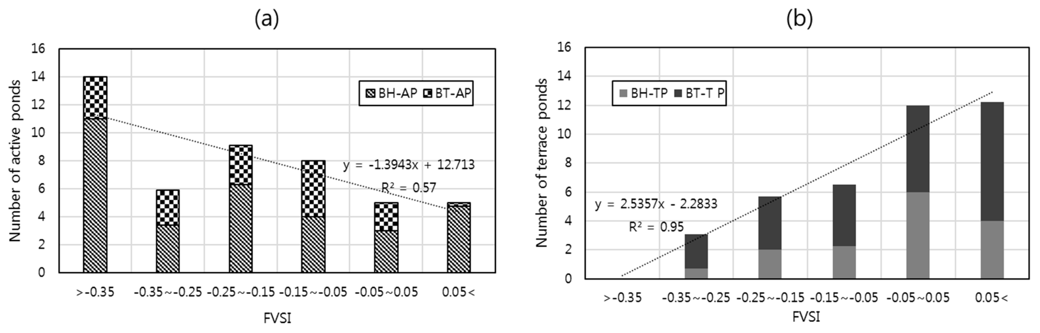
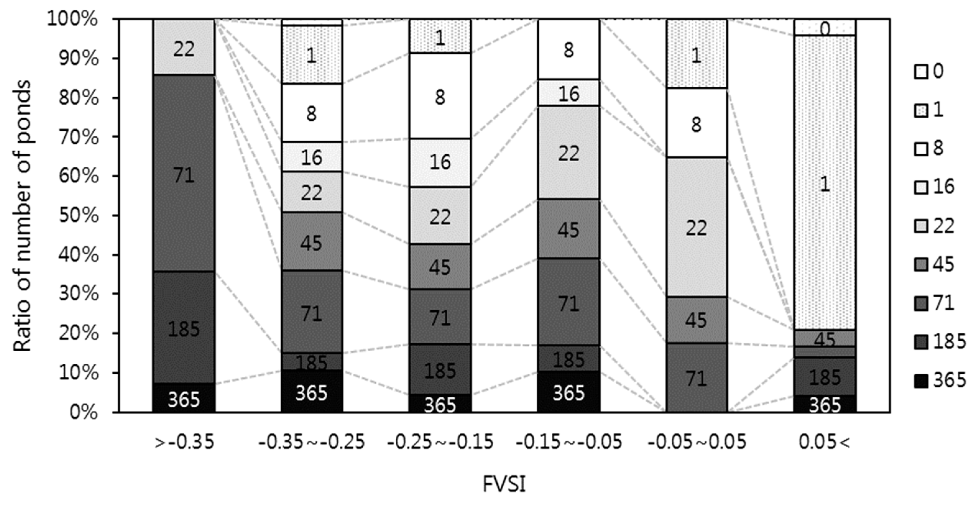
3.3. Relationship between the Habitat Structures and FVSI

FVSI was classified into six groups (Figure 10). The number of ponds was counted by considering the categorized values of FVSI (Figure 9a), and ratio of ponds with different flooding frequencies was measured by FVSI (Figure 9b). All the ponds detected in aerial photos (n = 386), including 120 surveyed ponds, were used in this relationship. Reaches with FVSI values of less than −0.35 had a high number of APs (Figure 10a), adversely those of more than 0.05 had high TPs (Figure 10b). Based on the increase in FVSI values, the number of APs decreased, whereas the number of TPs increased. The ratio of ponds with flooding frequencies is depicted in Figure 11. The ratio of ponds with a flooding frequency of 1 day/year significantly increased in reaches with FVSI exceeding 0.05. However, ponds with flooding frequencies of less than 16 days/year were not observed in the case of an FVSI of less −0.35. BH-TP and BH-TP with a flooding frequency of 8 days/year and 16–22 days/year exhibited that excellent suitability tended to exist for bitterlings and mussels on a reach with an FVSI that was between −0.35 and 0.05.

4. Discussion

4.1. Relationships among Species Abundance and Habitat

We attempted to understand the relationships between bitterlings/mussels and habitat structures with flooding frequency. Further, to explain the effect of habitat structures and flooding frequency on the habitat conditions, and relationships between habitat structures and habitat conditions were analyzed. Relationships between bitterling and chlorophyll tended be positive, even though the suitability of the bitterling in chlorophyll over 500 was very low (Table 1; Figure 6b). According to relationship between chlorophyll and habitat structures with flooding frequency, terrace pond with flooding frequency of 1–16 days/year showed relatively high chlorophyll (Figure 8b). Among these ponds, terrace ponds with flooding frequency of 8–16 days/year had high a HSI of bitterlings (Figure 7a). That is, suitability of bitterling had the high values in terrace ponds with a flooding frequency of 8–16 days/year, because they had a high value of chlorophyll that were positively related with bitterling. As the flooding frequency increases, the values of chlorophyll decreases. Maybe this is because frequent flooding reduces the residence time of water [21]. The infrequent flooding of ponds tended to maintain concentration of chlorophyll, and thus tended to influence bitterling habitat. A previous study [31] on CCA analysis between bitterlings/mussels and habitat conditions also showed that these species and chlorophyll have positive relationships.

The bitterling Acheilognathus longipinnis is listed on the IUCN red species and is a domestic species with national monument in Japan. However, this bitterling has not been found in the Yodo River system since 2006 [32]. The Kizu River joins the Yodo River. Therefore, the Yodogawa River Bureau and Osaka-fu prefecture implemented the re-introduction of the bitterling Acheilognathus longipinnis in the autumn of 2009 as an experimental trial. Mature adults (five hundred individuals) were released into embayments of the Yodo River in autumn 2009 during the spawning season. A total of 133 juveniles were observed in the embayments, but no juveniles were found in the spring of 2011. The bitterling restoration project continues, and this paper could be support of this restoration project.

Mussels were negatively related to the mud depth (Table 1; Figure 6b). Mussels also were more clearly observed in TPs than APs, especially the TPs located in the lower area of bars with a flooding frequency of 8 days/year and those located in the upper area of bars with flooding frequencies of 16–22 days/year than in APs (Figure 7b). Further, these TPs had an average mud depth of 1 cm (Figure 8c). Mussels require an appropriate depth of sediments under stable conditions because they live buried in the riverbed [21], and they filter the surrounding water to obtain food and oxygen [33]. However, deep mud may influence negative relationships with mussels, as shown in Figure 6c. Here, the pond is generated by erosion during large flood events, and is sustained by frequent intermediate flood events. In the case of TPs, the depth of the mud is likely to deepen by the deposition of suspended load by frequent intermediate flood events. Therefore, in the case of BT-TP, a flooding frequency of 16–22 days exhibits considerable mud depth as compared to that obtained at a flooding frequency of 1–8 days. If the mud depth increases, mussels buried in the mud will find it difficult to breathe owing to the reduction in DO. The authors of Reference [21] explained that the survival rates of mussels were low and that the growth was approximately zero in infrequently inundated water bodies (backwater, wetlands) by conducting field-earing experiments in the case of the Kiso River, because infrequently inundated water bodies exhibited hypoxic conditions in substratum-water. Further, other studies [29,30] indicated that the sand size of substrate is more suitable than that of silt (fine size) or gravel (larger size). However, fine substrate sediments have been reported to increase the mortality rate in some freshwater mussel species [34]. We assumed that the mud depth until 1 cm could maintain suitable DO for mussel breathing; if the depth is increased, it could become difficult for mussels to live in the Kizu River.

Further, we detected that, although the same TP with the same flooding frequency, they showed different habitat conditions and abundance of mussels. The mud depth of BH-TP was lower than that observed in BT-TP by considering the same flooding frequency. Thus, the HSI of mussels belonging to BH-TP exhibited higher values as compared to that exhibited by BT-TP with a flooding frequency of 16–22 days. However, we were unable to explain the reason for this difference. We inferred that ponds located on the upper area in the bar have much more powerful river strength than ponds located in the lower area in the flood event. Further, the accumulation of chlorophyll and mud in ponds is prevented by tractive force. In future studies, we should perform various other comparative analyses and include hydraulic aspects.

4.2. Relationships between Habitats Structures and FVSI

FVSI reflects the channel configuration in the Kizu River. The concave reaches with an FVSI < −0.35 had a lot of ponds with frequent flooding frequency more than 22 days/year (Figure 11) and only active ponds (Figure 10b). This indicates the significantly concave reaches with FVSI < −0.35 had low habitat suitability for bitterlings and mussels, because they have few suitable habitat structures (terrace ponds) with flooding frequency (8–22 days/year). These reaches were related with wandering, bifurcated, and braided channels in the Kizu River (Figure 5). Their floodplain is frequently inundated, and thus active channel was wide and area of vegetation was small. Hence, active ponds or backwaters on active channels are mainly located on these reaches. Although these channel types may have low potential of bitterlings and mussels, they may have high potential for other fish or aspects of lotic habitats. For example, Sukhodolov et al. and, Payne and Lapointe [15,16] noted that braided channels supply suitable conditions for fish shelters in terms of depth and velocity. Choi et al. [13] also examined that the bifurcated channel exhibits higher habitat diversity for both lentic and lotic habitats as compared to that exhibited by the single or slightly wandering channels. Since this study focused on lentic habitat with bitterlings and mussels, channel types with FVSI < −0.35 tended to have lower potential than others.

On the other hand, the convex channel reaches with an FVSI > 0.05 had a lot of terrace ponds with infrequent flooding frequency (1 day/year). Although habitat with infrequent flooding was suitable for bitterlings and mussels in the Kizu River, less flooding about 1 day/year showed the low suitability for bitterlings and mussels (Figure 7). However, unfortunately, there was no clear difference of environmental conditions between flooding frequency of 1 day and others (8, 16, 22, 45, 71, 185, and 365 days), and between active ponds and terrace ponds in the same flooding frequency 1 day.

Therefore, the intermediate channel types tended to be suitable excluding reaches of significant concave floodplain vertical shape (FVSI < −0.35) and convex shape (FVSI > 0.05). These suitable reaches were related to single or slightly wandering channels in the Kizu River (Figure 5), and these reaches were detected more after the 1990s (Figure 9). Similarly, studies related to the potential of recent channel conditions of the Kizu River were also noted by Reference [35]. They classified riffle structures into four types (traverse, converge, diverge I and II types), and surveyed the biomass and taxonomic richness of invertebrates per these riffle types. Further, the areas of each riffle type were measured using aerial photos that were obtained over 65 years. Their results exhibited that traverse and converge types of riffle had more biomass and taxonomic richness of invertebrates as compared to the diverge types; further, the areas of these riffle types increased after the 1970s. They discussed that river conditions from the 1980s to the 2010s may have had more biomass and richness than before. Thus, we recommend establishing countermeasures to prevent an increase in single or slightly wandering channel types to an FVSI of more than 0.05 to include many ponds with a flooding frequency of 1 day/year rather than restoring the previous channel conditions.

4.3. Application of FVSI to Sediment Management

Dam constructions cause the regular flow and the reduction of sediment transport. Stabilized flow and low sediment volume results in channel changes from braided (mobile) channel to single or single-thread (stabilized) channels [36]. In the Kizu River, these channel changes occurred over 60 years [13] with a reduction of sediment transport (Figure 2). A stabilized channel shows channel narrowing and incision with vegetation encroachment [2]. The encroachment of riparian vegetation into high level of floodplain by reduction in flood scour and sediment deposition is related to the high value of floodplain vertical shape index. As sediment deposition and vegetation expansion lead to an increase in the relative elevation of floodplains, FVSI was calculated by difference between elevation of floodplain and water level in main channel increases. Thus, positive values (convex shape) of FVSI meant stabilized channel such as single or semi wandering channels, and negative values (concave shape) meant more mobile channels such as wandering, bifurcated and braided channels in the Kizu River (Figure 5). This means that a greater reduction of sediment transport could further increase the FVSI. Therefore, sediment supplies need to maintain the current channel condition, not the more stabilized channel, for bitterlings and mussels. If we want to maintain single or slightly wandering channels with FVSI less than 0.05, we could consider a suitable period as between 1990s and 2000s (Figure 9), and suggest the volume of sediment transport at the time (20,000–50,000 m³/y) of sediment management. However, this is an indirect and long-term measurement. The consideration of various external and internal conditions should precede before the management.

On the other hand, the sediment management such as replenishment directly leads to improved habitat quality. The sediment excavated at the upstream of dam was moved to downstream by dump truck or other transportation [5]. Then, the riverbed was reformed by magnitude or duration of flushing flow or natural flood. Kondolf [2] stated that sediment supply contributed to enhancing the available spawning habitat for chinook salmon. Wood and Armitage [6] said that replenishment of coarse sediment increased the lotic habitat quality for invertebrates and fishes. Additionally, it is possible to convey sediment from convex floodplain vertical shape (FVSI greater than 0.05 having low potential of bitterlings and mussels) to significant concave floodplain vertical shape (FVSI less than −0.35 having low potential of bitterlings and mussels). The area of convex floodplain vertical shape requires a reduction of sediment deposition on the floodplain for changing the movable channels, and significant concave floodplain vertical shape requires sediment deposition for changing the stabilized channel. These processes could be predicted through simulations or experiments. The experiments and simulations of the sediment replenishment had been undertaken in tributary of the Kizu River [5]. However, ecological evaluation of the sediment management has not yet been properly performed. This study tried to support ecological connectivity between species abundance and sediment management based on relationships among animal communities, habitat structures with flooding frequency, and channel characteristics.

5. Conclusions

The reach-scale channel characteristics helped to determine a suitable target image for ecological sediment management on a catchment scale based on the multiscale relationships. The bitterlings and mussels were more abundant in terrace ponds than in active ponds, especially terrace ponds with a flooding frequency of 8–22 days/year. These suitable pond types tended to be located on the reaches with floodplain vertical shape index between −0.35 and 0.05 under the current channel conditions in the Kizu River. Thus, we recommend establishing long-term countermeasures of required sediment volume to maintain current conditions at sediment supply downstream. In terms of short-term countermeasures, we could suggest the target conditions at experiments and simulation of sediment replenishment. Although this study is based on a simple relationship analysis and requires considerably detailed correlation analysis, it could indicate an eco-geomorphic framework for river management based on the hierarchical interrelationships. In future, we will supplement the biological characteristics of bitterlings and mussels and various habitat conditions based on the hydraulic interpretation.

References

1. Kondolf, G.M.; Gao, Y.; Annandale, G.W.; Morris, G.L.; Jiang, E.; Zhang, J.; Cao, Y.; Carling, P.; Fu, K.; Guo, Q.; et al. Sustainable sediment management in reservoirs and regulated rivers: Experiences from five continents. Earth’s Future 2014, 2, 256–280. [Google Scholar] [CrossRef]
2. Kondolf, G.M. Hungry Water: Effects of Dams and Gravel Mining on River Channels. Environ. Manag. 1997, 21, 533–551. [Google Scholar] [CrossRef]
3. Auel, C.; Kobayashi, T.; Takemon, Y. Effects of sediment bypass tunnels on sediment grain size distribution and benthic habitats. Int. J. River Basin Manag. 2017, 15, 433–444. [Google Scholar] [CrossRef]
4. Kantoush, S.A.; Sumi, T.; Kubota, A. Geomorphic response of rivers below dams by sediment replenishment technique. In River Flow 2010; Dittrich, A., Koll, K., Aberle, J., Geisenhainer, P., Eds.; Bundesanstalt für Wasserbau: Karlsruhe, Germany, 2010; pp. 1155–1163. [Google Scholar]
5. Ock, G.; Sumi, T.; Takemon, Y. Sediment replenishment to downstream reaches below dams: Implementation perspectives. Hydrol. Res. Lett. 2013, 7, 54–59. [Google Scholar] [CrossRef]
6. Wood, P.J.; Armitage, P.D. Biological effects of fine sediment in the lotic environment. Environ. Manag. 1997, 21, 203–217. [Google Scholar] [CrossRef]
7. Leopold, L.B.; Wolman, M.G. River Channel Patterns: Braided, Meandering and Straight; US Geological Survey Professional Paper; U.S. Government Printing Office: Washington, DC, USA, 1957; Volume 282B, pp. 39–85.
8. Schumm, S.A. Patterns of alluvial rivers. Annu. Rev. Earth Planet. Sci. 1985, 13, 5–27. [Google Scholar] [CrossRef]
9. Rosgen, D.L. A classification of natural rivers. Catena 1994, 22, 169–199. [Google Scholar] [CrossRef] [Green Version]
10. Brierley, G.; Fryirs, K. Geomorphology and River Management: Applications of the River Styles Framework; Blackwell: Oxford, UK, 2005. [Google Scholar]
11. Wheaton, J.M.; Brasington, J.; Darby, S.E.; Merz, J.; Pasternack, G.B.; Sear, D.; Vericat, D. Linking geomorphic changes to salmonid habitat at a scale relevant to fish. River Res. Appl. 2010, 26, 469–486. [Google Scholar] [CrossRef]
12. Wyrick, J.R.; Pasternack, G.B. Geospatial organization of fluvial landforms in a gravel-cobble river: Beyond the riffle-pool couplet. Geomorphology 2014, 213, 48–65. [Google Scholar] [CrossRef]
13. Choi, M.; Takemon, Y.; Yu, W.; Jung, K. Ecological evaluation of reach scale channel configuration based on habitat structures for river management. J. Hydroinform. 2018, 20, 622–632. [Google Scholar] [CrossRef]
14. Frothingham, K.M.; Rhoads, B.L.; Herricks, E.E. A multiscale conceptual framework for integrated eco-geomorphological research to support stream naturalization in the agricultural Midwest. Environ. Manag. 2002, 29, 16–23. [Google Scholar] [CrossRef]
15. Sukhodolov, A.; Bertoldi, W.; Wolter, C.; Surian, N.; Tubino, M. Implication of channel processes for juvenile fish habitats in Alpine rivers. Aquat. Sci. 2009, 71, 338–349. [Google Scholar] [CrossRef]
16. Payne, B.A.; Lapointe, M.F. Channel morphology and lateral stability: Effects on distribution of spawning and rearing habitat for Atlantic salmon in a wandering cobble-bed river. Can. J. Fish. Aquat. Sci. 1997, 54, 2627–2636. [Google Scholar] [CrossRef]
17. Beechie, T.J.; Liermann, M.; Pollock, M.M.; Baker, S.; Davies, J. Channel pattern and river-floodplain dynamics in forested mountain river systems. Geomorphology 2006, 78, 124–141. [Google Scholar] [CrossRef]
18. Tockner, K.; Ward, J.V.; Arscott, D.B.; Edwards, P.J.; Kollmann, J.; Gurnell, A.M.; Petts, G.E.; Maiolini, B. The Tagliamento River: A model ecosystem of European importance. Aquat. Sci. 2003, 65, 239–253. [Google Scholar] [CrossRef]
19. Arscott, D.B.; Tockner, K.; van der Nat, D.; Ward, J.V. Aquatic Habitat Dynamics along a Braided Alpine River Ecosystem (Tagliamento River, Northeast Italy). Ecosystems 2002, 5, 802–814. [Google Scholar] [CrossRef]
20. Kizu River Research Group. Integrated Research of the Kizu River II; Kizu River Research Group: Kyoto, Japan, 2003. (In Japanese) [Google Scholar]
21. Negishi, J.N.; Sagawa, S.; Kayaba, Y.; Sanada, S.; Kume, M.; Miyashita, T. Mussel responses to flood pulse frequency: The important of local habitat. Freshw. Biol. 2012, 57, 1500–1511. [Google Scholar] [CrossRef]
22. Takemon, Y.; Kobayashi, S.; Choi, M.; Terada, M.; Takebayashi, H.; Sumi, T. River Habitat Evaluation based on Cross-sectional Bed Profile and Frequency Distribution of Relative Elevation. Adv. River Eng. 2013, 19, 519–524. (In Japanese) [Google Scholar]
23. Egashira, S.; Jin, H.; Takebayashi, H.; Nida, B.; Nagata, T. Bed variation and sediment budget in the downstream reach of Kizu River. Annu. J. Hydraul. Eng. 2002, 44, 777–782. (In Japanese) [Google Scholar] [CrossRef]
24. Jowett, I.G.; Davey, A.J.H. A Comparison of Composite Habitat Suitability Indices and Generalized Additive Models of Invertebrate Abundance and Fish Presence-Habitat Availability. Trans. Am. Fish. Soc. 2007, 136, 428–444. [Google Scholar] [CrossRef]
25. Bovee, K.D. Development and Evaluation of Habitat Suitability Criteria for Use in the Instream Flow Incremental Methodology; National Ecology Center, U.S. Fish and Wildlife Service: Washington, DC, USA, 1986. [Google Scholar]
26. Survey Report on the Kizu River; Yodogawa River Bureau, ASIA AIR SURVEY CO., LTD.: Osaka, Japan, 2007. (In Japanese)
27. Survey Report on the Kizu River; Yodogawa River Bureau, ASIA AIR SURVEY CO., LTD.: Osaka, Japan, 2009. (In Japanese)
28. Survey Report on the Kizu River; Yodogawa River Bureau, ASIA AIR SURVEY CO., LTD.: Osaka, Japan, 2010. (In Japanese)
29. Johnson, P.D.; Brown, K.M. The importance of microhabitat factors and habitat stability to the threatened Louisiana pearl shell, Mrgaritifera hembeli (Conrad). Can. J. Zool. 2000, 78, 271–277. [Google Scholar] [CrossRef]
30. Yoshihiro, B.A.; Takashi, M. Habitat Characteristics Influencing Distribution of the Freshwater Mussel Pronodularia japanensis and Potential Impact on the Tokyo Bitterling, Tanakia tanago. Zool. Sci. 2010, 27, 912–916. [Google Scholar]
31. Terada, M.; Takemon, Y.; Sumi, T. A study on habitat evaluation of tamari for bitterling and mussel. In Proceedings of the JSCE-Kansai, Uji, Japan, 26 August 2011; Volume II-12. (In Japanese). [Google Scholar]
32. Global Re-introduction Perspectives: 2011; IUCN/SSC Re-Introduction Specialist Group: Calgary, AB, Canada, 2011.
33. Reichard, M.; Liu, H.; Smith, C. The co-evolutionary relationship between bitterling fishes and freshwater mussels: Insights from interspecific comparison. Evolut. Ecol. Res. 2007, 9, 239–259. [Google Scholar]
34. Ellis, M.M. Erosion silt as a factor in aquatic environments. Ecology 1936, 17, 29–42. [Google Scholar] [CrossRef]
35. Kobayashi, S.; Takemon, Y. Historical Changes of Riffle Morphology for Benthic Invertebrate Habitats in the Kizu River. Annu. Disaster Prev. Res. Inst. Kyoto Univ. 2013, 56B, 681–689. (In Japanese) [Google Scholar]
36. Surian, N.; Rinaldi, M. Morphological response to river engineering and management in alluvial channels in Italy. Geomorphology 2003, 50, 307–326. [Google Scholar] [CrossRef] [Green Version]
Figure 1. Study site in the Kizu River.
Water 10 01479 g001
Figure 2. Historic changes in annual transport sediment volume in the Kizu River were estimated in Reference [23].
Water 10 01479 g002
Figure 3. Lentic habitats and target species. (a) Image showing classification of lentic habitats; (b) an active pond (AP); (c) a terrace pond (TP); (d) bitterling; and (e) mussel.
Water 10 01479 g003
Figure 4. (a) Calculation of the floodplain vertical shape index (FVSI); (b) a positive value indicates a convex floodplain vertical shape; and (c) a negative value indicates a concave vertical shape.
Water 10 01479 g004
Figure 5. Classification of the channel configurations in the Kizu River [13] and their relationship with FVSI. The squares of FVSI indicate the average FVSI value per channel type (mean ± SE). Similar letters above histograms indicate significant differences based on Tukey’s tests.
Water 10 01479 g005
Figure 6. Habitat Suitability Index (HSI) values with habitat conditions were selected for the best models. The HSI of bitterlings and habitat conditions of (a) dissolved oxygen (DO) (mg/L) and (b) Chlorophyll (μg/L). The HSI of mussels and habitat condition of (c) mud depth (cm) and (d) wood coverage (%).
Water 10 01479 g006
Figure 7. HSI of (a) bitterlings and (b) mussels, and habitat structures with the flooding frequency. Habitat structures are: BH-AP (bar head-active pond), BH-TP (bar head-terrace pond), BT-AP (bar tail-active pond), and BT-TP (bar tail-terrace pond).
Water 10 01479 g007
Figure 8. Relationships between the average habitat conditions: (a) DO; (b) chlorophyll; (c) mud depth; and (d) wood coverage and habitat types with flooding frequency. Habitat structures are: BH-AP (bar head-active pond), BH-TP (bar head-terrace pond), BT-AP (bar tail-active pond), and BT-TP (bar tail-terrace pond).
Water 10 01479 g008
Figure 9. Historical changes in FVSI. Since the study area extends to a length of 26 km, 12 FVSI values per year obtained. The squares indicate the annual average.
Water 10 01479 g009
Figure 10. Relationships between the number of habitat types with (a) active ponds and (b) terrace ponds and FVSI. Habitat structures are: BH-AP (bar head-active pond), BH-TP (bar head-terrace pond), BT-AP (bar tail-active pond), and BT-TP (bar tail-terrace pond).
Water 10 01479 g010
Figure 11. Relationships between the ratio of flooding frequency of habitat and FVSI.
Water 10 01479 g011