Analysis of Flood Risk of Urban Agglomeration Polders Using Multivariate Copula

Abstract

Urban agglomeration polders (UAPs) are often used to control flooding in eastern China. The impacts of UAPs on individual flood events have been extensively examined, but how flood risks are influenced by UAPs is much less examined. This study aimed to explore a three-dimensional joint distribution of annual flood volume, peak flow and water level to examine UAPs’ impact on flood risks based on hydrological simulations. The dependence between pairwise hydrological characteristics are measured by rank correlation coefficients and graphs. An Archimedean Copula is applied to model the dependence structure. This approach is applied to the Qinhuai River Basin where UAPs are used proactively for flood control. The result shows that the Frank Copula can better represent the dependence structure in the Qinhuai River Basin. UAPs increase risks of individual flood characteristics and integrated risks. UAPs have a relatively greater impact on water level than the other two flood characteristics. It is noted that the impact on flood risk levels off for greater floods.

1. Introduction

In the plain region of eastern China, urbanization has been developing rapidly for decades [1,2]. In order to protect life and property [3], polders have been built in cities in the regions which include Suzhou, Wuxi, Changzhou and Jiaxing in the Yangtze River Delta plain, and Nanjing, Jurong and Lishui in the Qinhuai River Basin, a tributary of the lower Yangtze River. With embankment, sluice controls and drainage stations, polders can control external floods and drain excessive water that is within its range [4]. After the catastrophic floods in 1954, 1991 and 1998, dikes continue to be strengthened and raised, and flood control standards have been gradually increased. In some cities, such as Nanjing, dikes even can control the 100-year flood. These dikes and embankments are "heroes" for controlling external floods, but they are also “time bombs” placed next to cities. For example, during the catastrophic flood in the Yangtze River in 1998 [5], the Yangtze River embankment in Jiujiang City breached due to high water levels, outflows of the Poyang Lake, and most primarily infiltration damages to the embankment basement. As a result, the entire city was faced with the risk of being engulfed by floods.

With the increasing flood control capacity within polders, excess water can be drained to the rivers out of polders in a relatively short period of time [6], resulting in soaring river water levels and in return increasing the flood risks of the polder area and even the entire basin [7,8]. Considering flood changes with urban polders, Xing et al. [9] calculated the risk factor of hydrological failure for levees of the external Qinhuai River. Xu et al. [10] proposed a method to determine waterlogging risks for river basins with polders based on analysis of flood characteristics. Zhao et al. [11] studied the accident risk analysis method for dikes. Zhang [12] analyzed the influence of polders, which were completed as joint river embankments for the period of the 1950s to the 1970s, on storage capacity and ecological environment in the Taihu Lake Basin. Xu et al. [13] analyzed the change of river network structure caused by polders using GIS and RS. Yuan et al. [14] simulated flood events in the Qinhuai River Basin with an HEC-HMS hydrological model and analyzed the influence of polder features on flood control. Chen et al. [15] established a comprehensive evaluation model to analyze the waterlogging risks of farm lands under the current situation and various scenarios with polder construction in Yundong District, Gaoyou, China. However, there is little research on flood risks caused by polders, and most of the research on flood risks is limited to a single factor. Therefore, based on the previous work of the HEC-HMS hydrological model and an HEC-RAS hydraulic model developed by Yuan et al. [14], the impact on flood risks by developing polders are examined using the hydrological and hydraulic simulation results.

2. Materials and Methods

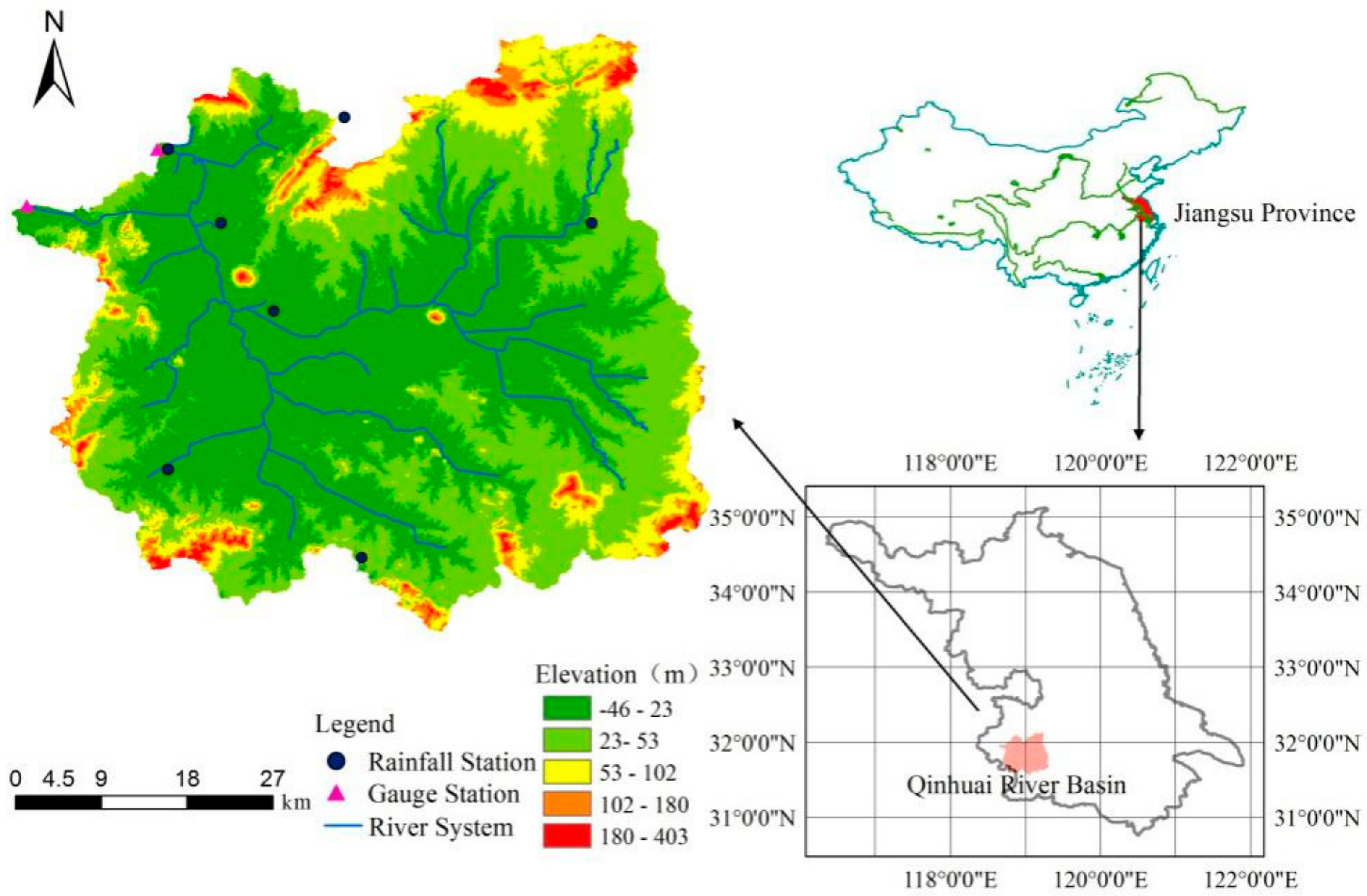
2.1. Study Area and Data

The Qinhuai River Basin (Figure 1) is located in the lower Yangtze River with a total drainage area of 2631 square kilometers, between the latitude of 28–31° N and the longitude of 118–121° E. It lies in the subtropical humid and semihumid monsoon climate region, with an average annual precipitation of 1047 mm and an average annual temperature of 15.4 °C. The precipitation gradually increases from north to south and the intra-annual temperatures vary greatly. The land-use types are primarily paddy field, and secondly, dry land and urban land, accounting for 62.4%, 23.3% and 5.6% of the total drainage area, respectively.

Cities in the Qinhuai River Basin construct their own polders on the basis of expanding and adjusting protection areas in the basin. A total of six flood control polders had been built in the basin by 2016. Based on the geographic proximity, four UAPs are identified as the Jurong and Lishui polders in the upper reach, the Qianhancun polder in the middle reach and the Dongshan polder in the lower reach. The geographic distribution of the four UAPs is shown in Figure 2. The total protection area is 872.4 km², accounting for more than 60% of the entire drainage area. Due to increasing polders, river network density and network complexity have showed downward trends, and water levels are continuously rising. According to historical data, floods in the main stem of the Qinhuai River kept reaching new records, and flood stages in the Dongshan Station frequently exceeded the flood warning level. Water resources managers are faced with the challenge of increasing floods.

This paper studies the influence of UAPs on flood risks based on our previous hydrological and hydraulic simulations of the basin. Yuan et al. developed the HEC-HMS hydrological model and the HEC-RAS hydraulic model for the Qinhuai River Basin. Both models are well calibrated and validated. The three flood characteristics, that is, flood volumes, peak flows and flood levels, are selected to describe flood risk. Flood volumes and peak flows are calculated using the daily streamflow data for Wudingmen Station and Qinhuaixinhe Station, and the flood levels are measured for the Dongshan Station. A joint flood risk model considering flood volume, peak flow and flood level is developed to analyze flood risks and polders’ impacts on flood risks.

2.2. Methodology

2.2.1. Archimedean Copula

The Copula function can be used to describe dependencies of two or more variables, and there is no assumption on underlying marginal distribution of variables [16,17]. Assuming that variables $X_1,X_2,\dots ,X_m$ have marginal distributions as $F_{X_1},F_{X_2},\dots ,F_{X_m}$ and their joint distribution is $F\left(X_1,X_2,\dots ,X_m\right)$, then the Copula function can be defined as

$$C\left(u_1,u_2,\dots ,u_m\right)=F\left(X_1,X_2,\dots ,X_m\right); u_k=F_{X_k}(X_k),u_k\in [0,1],k=1,2,\dots ,m$$

(1)

The Archimedean Copula is one of the most widely used Copula functions, mainly because of its small number of parameters, simple structure and clear expression. Generally, a one-parameter Archimedean Copula is symmetric, and a d-dimensional Copula C_d: (0,1)^d→(0,1) can be defined as:

$$C(u_1,u_2,\cdots ,u_d)={\phi }^{-1}\left[{\displaystyle \sum }_{k=1}^d\phi \left(u_k\right)\right]={\phi }^{-1}\left[\phi \left(u_1\right)+\phi \left(u_2\right)+\cdots \phi \left(u_d\right)\right],$$

(2)

$$u_k\in \left[0,1\right],k=1,\cdots ,d,$$

where $\phi (·)$ is the generating function of the Archimedean Copula, and ${\phi }^{-1}$ is the inverse function of $\phi$.

Common Archimedean Copulas include Gumbel-Hougaard, Clayton, and Frank Copula, and their functions are shown in

Table 1. Common Archimedean Copula functions [18,19,20].

Copula	Trivariate Coupla Function
GH	$C\left(u_1,u_2,u_3\right)=\exp \left(-{\left[{\left(-\ln \left(u_1\right)\right)}^{\mathsf{\theta }}+{\left(-\ln \left(u_2\right)\right)}^{\mathsf{\theta }}+{\left(-\ln \left(u_3\right)\right)}^{\mathsf{\theta }}\right]}^{\frac{1}{\mathsf{\theta }}}\right) \mathsf{\theta }\in \left(0,\infty \right)$
Clayton	$C\left(u_1,u_2,u_3\right)={\left(u_1{}^{-\mathsf{\theta }}+u_2{}^{-\mathsf{\theta }}+u_3{}^{-\mathsf{\theta }}-2\right)}^{-1/\mathsf{\theta }} \mathsf{\theta }\in \left(1,\infty \right)$
Frank	$C\left(u_1,u_2,u_3\right)=-\frac{1}{\mathsf{\theta }}\ln \left(1+\frac{(\exp \left(-\mathsf{\theta }{u}_1\right)-1)(\exp \left(-\mathsf{\theta }{u}_2\right)-1)(\exp \left(-\mathsf{\theta }{u}_3\right)-1)}{(\exp \left(-\mathsf{\theta }\right)-1)}\right)$

.

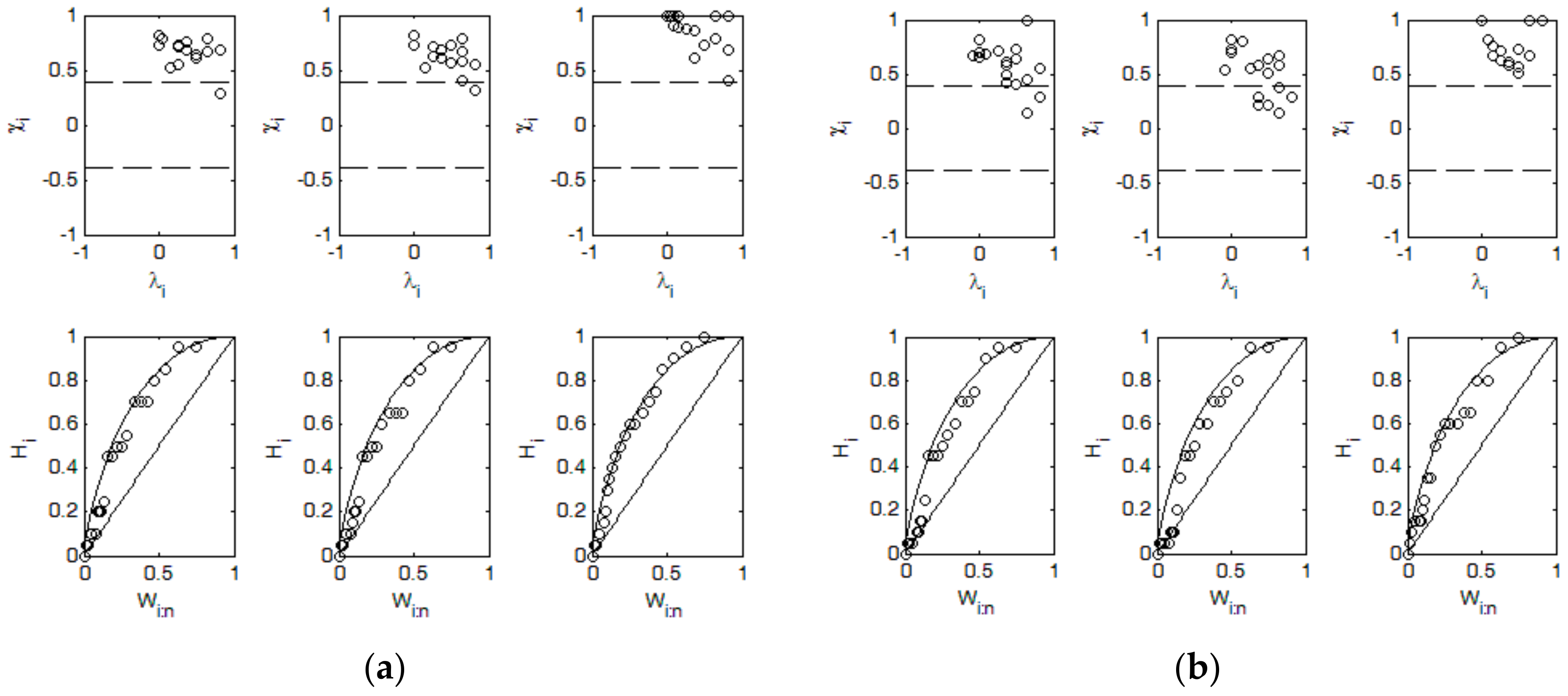
2.2.2. Dependence and Ranks

To measure the statistical dependence between random variables, two well-known nonparametric dependence measures, that is, the Spearman rank correlation coefficient (ρ) and Kendall rank correlation coefficient (τ), are used. The Spearman’s ρ and Kendall’s τ are calculated using ranking of variable values rather than actual values, so they are invariant under monotonic nonlinear transformations [21]. They are calculated as follows:

$$\rho =\frac{12}{n\left(n+1\right)\left(n-1\right)}{\displaystyle \sum }_{i=1}^n{R}_i{S}_i-3\frac{n+1}{n-1},$$

(3)

$$\tau =\frac{2}{n\left(n-1\right)}{\displaystyle {\sum }_{1\le i\le j\le n}}sign\left(\left(x_i-x_i\right)\left(y_i-y_j\right)\right),$$

(4)

where $R_i$ and $S_i$ denote the ranking of variable X and Y, respectively. Sign(x) is the indicator function, $sign\left(x\right)=1$ when x is positive, $sign\left(x\right)=-1$ when x is negative, $sign\left(x\right)=0$. when x equals zero.

Visual tools offer a qualitative and direct way to examine dependence. In addition, two rank-based graphical tools for detecting dependence are also employed in this paper, namely, chi-plots and K-plots [21,22,23].

• Chi-plot

The chi-plot, originally proposed by Fisher and Switzer (1985) [24], is a scatter plot of the data pair $\left({\lambda }_i,{\chi }_i\right)$. ${\lambda }_i$ and ${\chi }_i$ are calculated as

$${\lambda }_i=4sign\left(\left(F_i-0.5\right)\left(G_i-0.5\right)\right)max\left\{{\left(F_i-0.5\right)}^2,{\left(G_i-0.5\right)}^2\right\},$$

(5)

where

$$H_i=\frac{{{\displaystyle \sum }}_{j\ne i}I\left(x_j\le x_i,y_j\le y_i\right)}{n-1},$$

(6)

$$F_i=\frac{{{\displaystyle \sum }}_{j\ne i}I\left(x_j\le x_i\right)}{n-1},$$

(7)

$$G_i=\frac{{{\displaystyle \sum }}_{j\ne i}I\left(y_j\le y_i\right)}{n-1}, \mathrm{and}$$

(8)

where I is an indicator function and $n$ denotes the sample size. $i=1,2,\dots ,n$. The value of ${\lambda }_i$ measures the distance of the observed pair value $\left(x_i,y_i\right)$ from the center of the scatter plot, and ${\lambda }_i\in \left[-1,1\right]$. If X is positively associated with Y, ${\lambda }_i$ will tend to be positive. If X and Y are independent, it is expected that $H_i=F_i{G}_i$, then ${\chi }_i=0$. Therefore, values of ${\chi }_i$ that fall far from zero indicate a certain degree of association between two variables. To help identify such departures, the chi-plot also includes control limits drawn at ${\chi }_i=\pm c_p/\sqrt{n}$ where $c_p$ values are suggested by Fisher and Switzer [24]. The $c_p$ values of 1.54, 1.78 and 2.18 correspond to p-values of 0.9, 0.95 and 0.99, respectively. When the scatter points fall largely on the upper side of the control limits, it indicates positive dependence; whereas in the case of negative dependence, the scatter points are largely in the lower side of the control limits.

• K-plot

The K-plot, firstly proposed by Genest and Boies (2003) [25], is analogous to a QQ plot. The K-plot consists in plotting the data pairs $(H_{\left(i\right)},W_{i:n})$ for $i\in \left\{1,2,\dots ,n\right\}$. $H_{\left(i\right)}$ in abscissa is the order statistics of the random variable $H_i$ introduced in Section 2.2.2. As for $W_{i:n}$ in ordinate, it is the expected value of the $i$-th statistic from a random sample of size $n$ from a random variable $W=F\left(X,Y\right)=C\left(U,V\right)$. It is given by

$$W_{i:n}=n\left(\begin{array}{c}n-1\\ i-1\end{array}\right){{\displaystyle \int }}_0^{1}wk\left(w\right){\left\{K\left(w\right)\right\}}^{i-1}{\left\{1-K\left(w\right)\right\}}^{n-i}dw ,$$

(9)

where $K\left(w\right)=P\left(UV\le w\right)=w-wlog\left(w\right)$, $k\left(w\right)=\frac{dK\left(w\right)}{dw}$, $\left(\begin{array}{c}n-1\\ i-1\end{array}\right)$ is a binominal coefficient. A straight line across the main diagonal is superimposed on the graph to the case of independence, and a smooth curve $K\left(w\right)$ located above the straight is associated with perfect positive dependence. In case of perfect negative dependence, it is shown as a string of data points aligned on the x-axis.

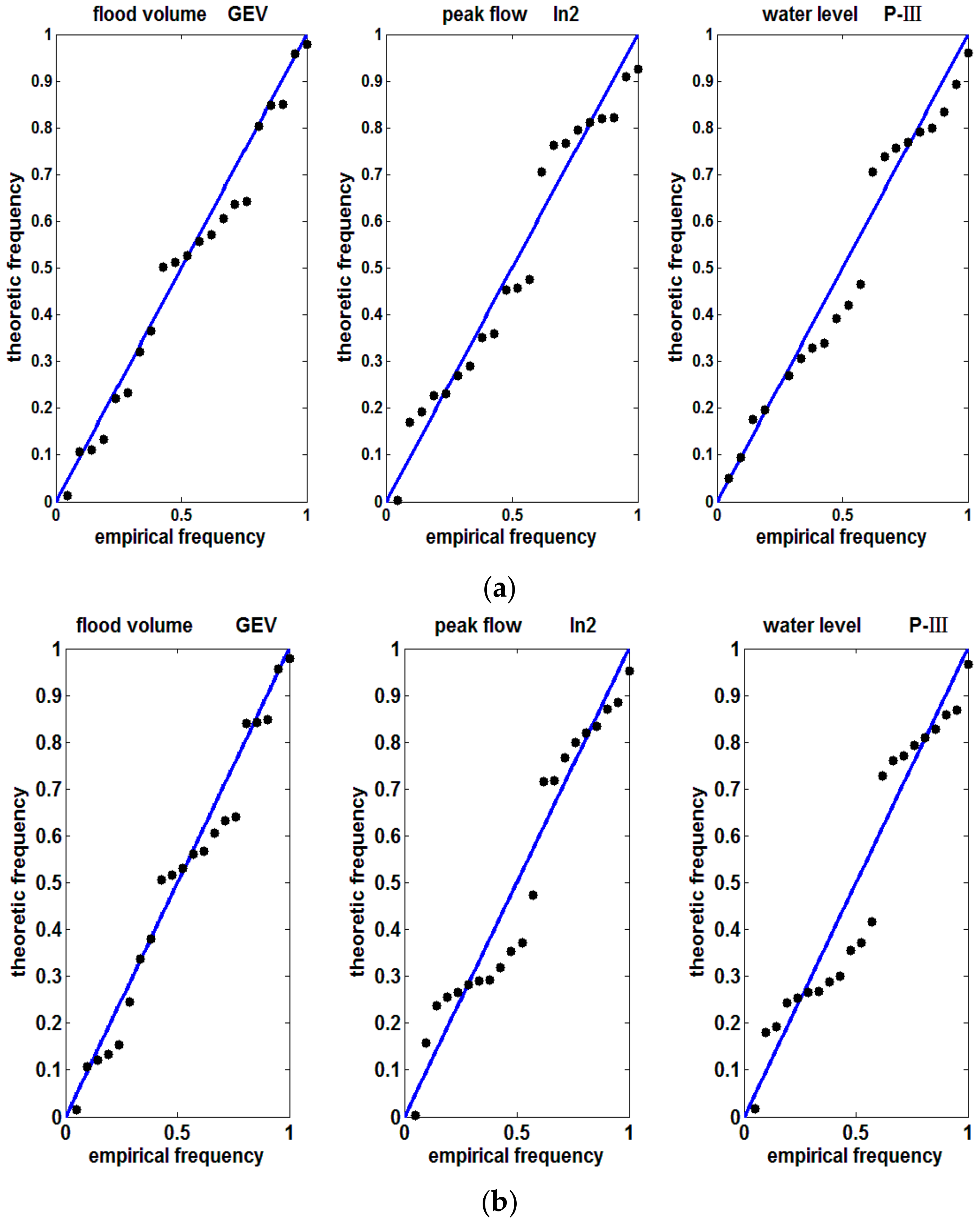
2.2.3. Goodness of Fit

The goodness of fit is examined with root-mean-square error (RMSE) and Akaike information criteria (AIC), two commonly used performance metrics [26].

RMSE is very sensitive to extremely large or small deviations between the theoretical value and the actual value, and it can represent the goodness of fit of a model. RMSE is calculated as follows:

$$RMSE=\sqrt{\frac{1}{n}{\displaystyle \sum }_{i=1}^n{(F\left(x_i\right)-F_0\left(x_i\right))}^2},$$

(10)

where F(x) is the theoretical distribution function; $F_0\left(x\right)$ is empirical distribution function; n is sample size; $MSE=E(F-F_0{)}^2=\frac{1}{n}{\displaystyle \sum _{i=1}^n}{[f\left(i\right)-f_0\left(i\right)]}^2$; and f and f₀ are the probability density functions of F and $F_0$, respectively.

AIC was proposed by a Japanese statistician Akira Hiroshi. It combines the maximum likelihood method with the maximum entropy principle to derive the selection criterion of the best model [17]. It is defined as:

$$AIC=n\ln \left(MSE\right)+2m,$$

(11)

where $MSE=E{(F-F_0)}^2=\frac{1}{n}{\displaystyle \sum _{i=1}^n}{[f\left(i\right)-f_0\left(i\right)]}^2$; m is the number of the Copula parameters; and f and f₀ are the probability density functions of F and $F_0$, respectively. The distribution function with better goodness of fit is selected by the minimum values of RMSE and AIC.

3. Results

3.1. Dependence of Flood Characteristics

Pair-wise dependence among the three flood characteristics, that is, flood volume (V), peak flow (P) and water level (Z), is shown in Appendix A

Table A1. Pair-wise dependence between flood characteristics.

Variable	With UAP		Without UAP
	Spearman	Kendall	Spearman	Kendall
V&P	0.921(4.5 × 10−6)	0.762(5.8 × 10−8)	0.877(9.5 × 10−7)	0.686(2.4 × 10−6)
V&Z	0.893(5.1 × 10−8)	0.73(4.4 × 10−6)	0.821(3.4 × 10−6)	0.619(3.2 × 10−5)
P&Z	0.974(1.2 × 10−13)	0.921(6.6 × 10−9)	0.926(4.7 × 10−6)	0.8(6.0 × 10−9)

, along with their corresponding p-values. Figure 3 presents chi-plots and K-plots of pair-wise flood characteristics for scenarios with and without polders. The dependence between pair-wise flood characteristics in the Qinhuai River Basin is strong, and the dependence between peak flow and water level (P&Z) is the strongest, which makes it reasonable to illustrate their joint probabilistic characterizations using a multivariate Copula function. For Figure 3a, data points are largely in the upper side of the control limits in the chi-plot or deviated from the main diagonal in the K-plot, confirming strong dependence among variables. The increased density of points close to the horizontal line of 1 in the upper-right corner in the chi-plot indicates strongest dependence between peak flow and water level (P&Z).

Comparing Figure 3a with Figure 3b, it can be easily seen that dependence among flood characteristics with UAPs is weaker than that without UAPs. It appears that the original river network is dissected by UAPs, and the hydraulic connectivity of the whole basin is decreased, which results in weaker dependence between flood characteristics.

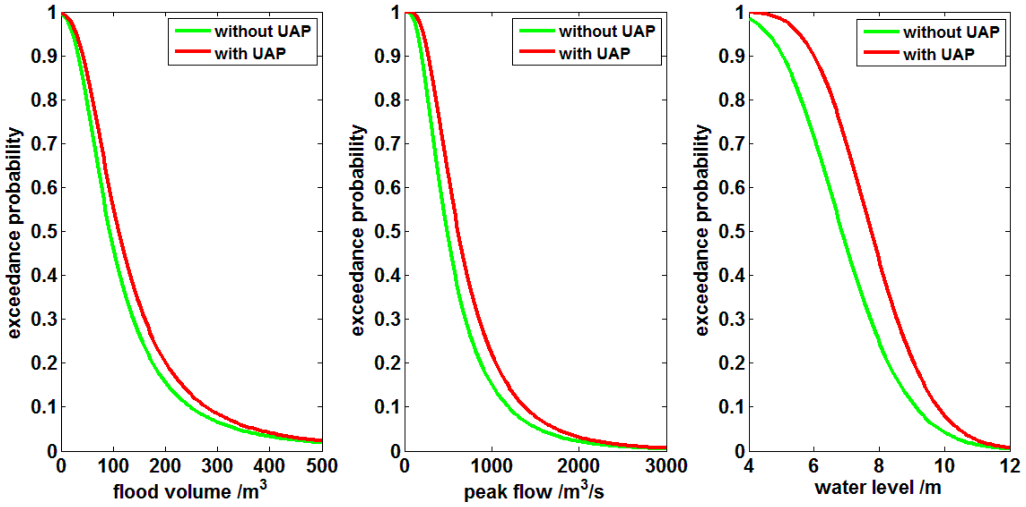
3.2. Marginal Distribution

The descriptive statistics for the flood characteristics of both scenarios with and without UAPs are shown in Appendix A

Table A2. Statistics of flood variables.

Statistics	Without UAP			With UAP
	V	P	Z	V	P	Z
Mean	126.03	591.21	6.99	143.99	729.01	7.84
Std.	112.81	350.50	1.45	118.17	419.10	1.41
Skewness	1.90	0.59	0.30	1.73	0.74	0.18
Kurtosis	6.20	2.32	2.20	5.64	2.72	2.32

. The skewness and kurtosis of flood volume is relatively obvious. To fit marginal functions to flood characteristics, three parametric distribution functions, namely the Pearson type three distribution (P-Ш), the generalized extreme value distribution (GEV) and the log-normal distribution (LN), are tested. The IFM method [27] is applied to estimate the parameters, and the KS test is conducted at a 5% significance level to determine the best-fitted function. The smaller the KS value, the better the fitting. The larger the p-value, the higher the chance that the distribution would be accepted. The results are shown in

Table 2. Parameter estimation and fitting performance of marginal distributions.

	PDF	Without UAPs (Urban Agglomeration Polders)					With UAPs (Urban Agglomeration Polders)
		Location	Scale	Shape	KS	P	Location	Scale	Shape	KS	P
V	P-Ш	28.38	0.004	0.44	0.23	0.20	14.40	0.006	0.83	0.20	0.34
	GEV	72.60	53.86	0.31	0.12	0.88	87.17	61.07	0.28	0.12	0.86
	LN	4.51	0.87	-	0.14	0.79	4.68	0.80	-	0.14	0.79
P	P-Ш	−247.93	0.006	4.63	0.15	0.71	32.16	0.003	2.16	0.16	0.56
	GEV	424.66	263.84	0.05	0.16	0.61	526.58	301.26	0.09	0.19	0.39
	LN	6.18	0.70	-	0.14	0.73	6.42	0.63	-	0.15	0.66
Z	P-Ш	0.56	2.49	16.00	0.14	0.79	−0.21	3.63	29.22	0.16	0.63
	GEV	6.42	1.29	−0.17	0.16	0.63	7.33	1.33	−0.24	0.17	0.49
	LN	1.92	0.21	-	0.16	0.63	2.04	0.18	-	0.17	0.54

. Based on the results, the best-fitted marginal distributions for flood volume, peak flow and water level, marked as bold, are chosen as GEV, LN and P-Ш, respectively. The marginal fitting results are the same for the scenarios with UAPs.

The correlation of empirical and theoretical frequency of marginal distribution is plotted in Figure 4. The points are positioned along the main diagonal 45° line, showing good fitting.

3.3. Joint Distribution

The marginal distributions for all three flood characteristics have been determined, and IFM is applied to estimate parameters of the Copula function. RMSE and AIC are used to test the goodness of fit. The results are shown in

Table 3. The goodness-of-fit test of joint distribution.

Copula	Without UAPs			With UAPs
	Theta	RMSE	AIC	Theta	RMSE	AIC
GH	3.680	0.015	−111.45	3.149	0.015	−111.42
Clayton	2.773	0.022	−94.58	2.463	0.018	−102.31
Frank	15.905	0.013	−117.43	14.040	0.014	−113.36

. Based on the results, the Frank Copula is chosen as the joint probability distribution to analyze integrated flood risk for scenarios with and without UAPs.

4. Discussion

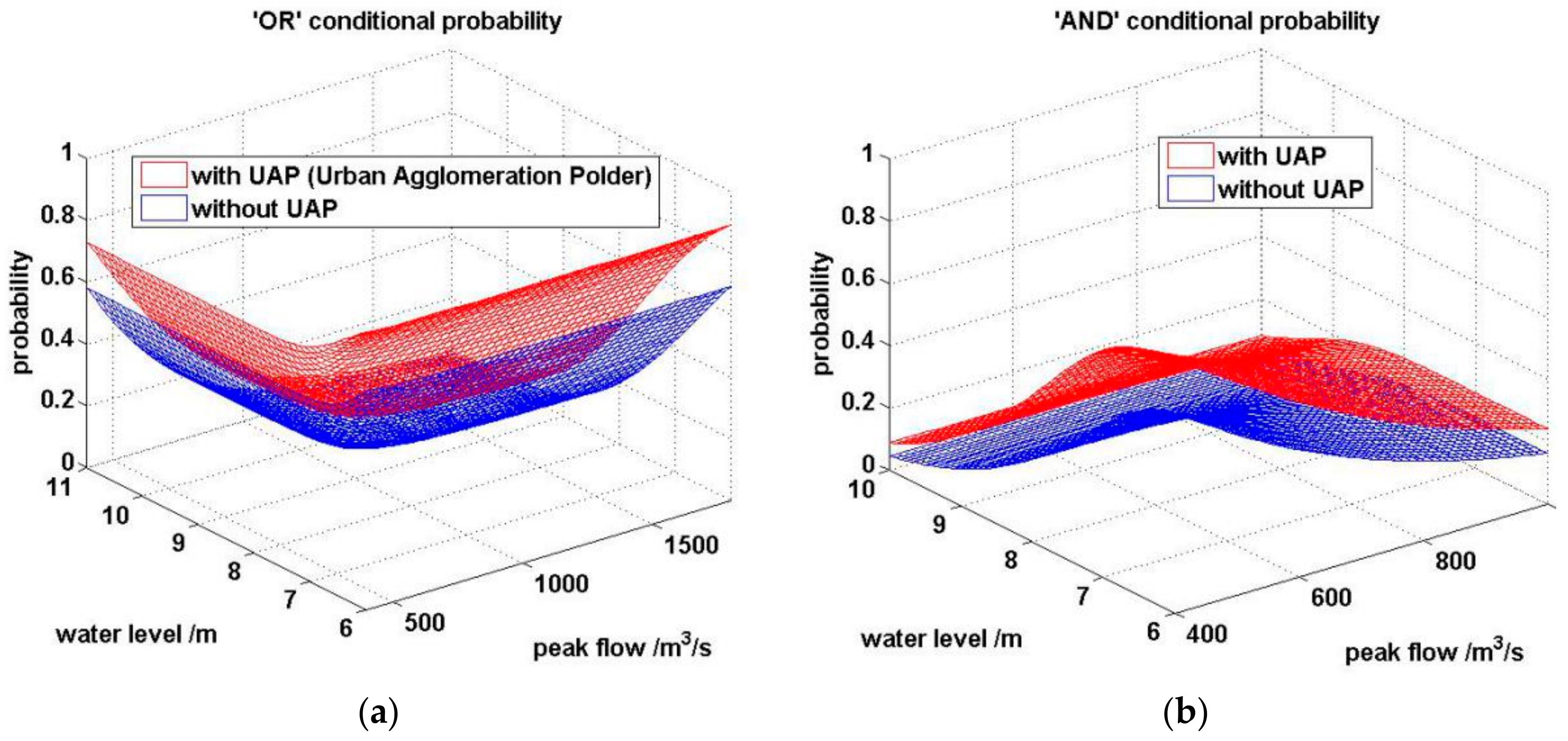
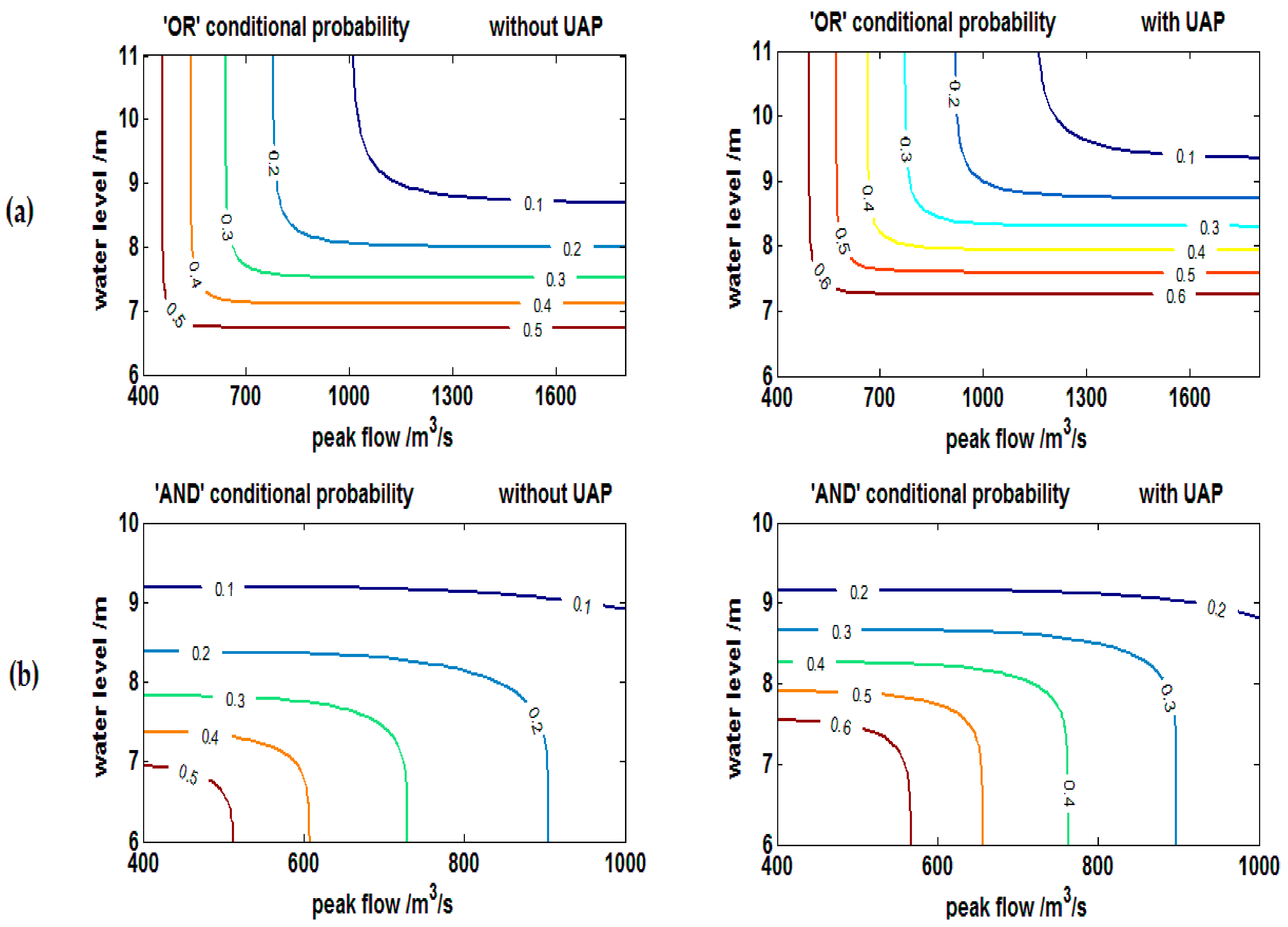
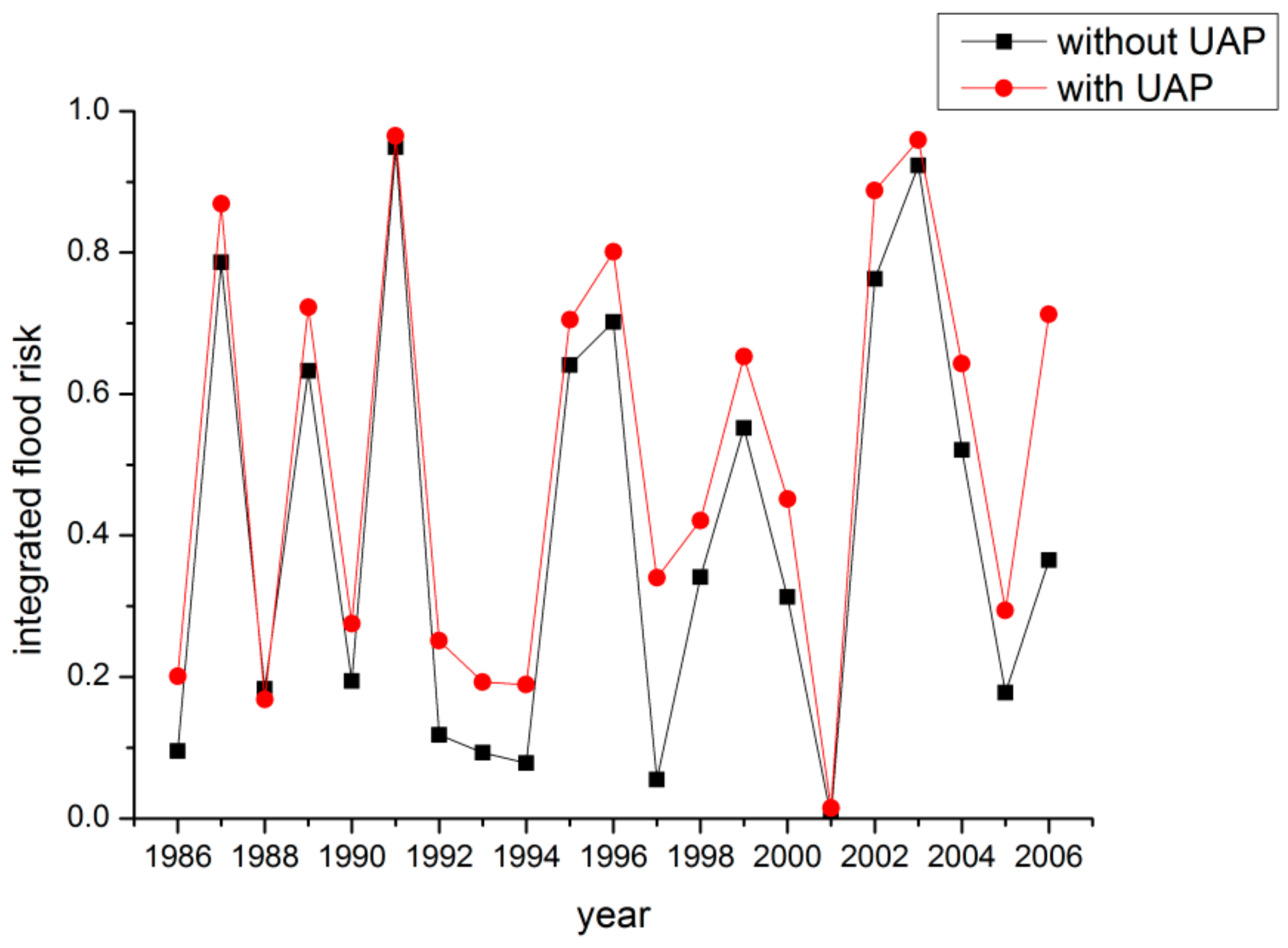
4.1. Impacts on Flood Risks of Polders

According to the identified marginal distributions and joint distribution, the design values for flood characteristics at different joint return periods (JRPs) are compared. The results are shown in

Table 4. Design value for flood characteristics.

JRP (/a)	Without UAPs			With UAPs
	V (m3)	P (m3/s)	Z (m)	V (m3)	P (m3/s)	Z (m)
10	331.03	1514.57	9.80	370.81	1738.81	10.40
20	473.94	2010.97	10.63	514.92	2232.61	11.13
50	702.69	2683.57	11.51	738.23	2884.44	11.89
100	914.87	3216.57	12.05	940.25	3392.11	12.35
200	1172.74	3783.76	12.55	1180.64	3925.00	12.74

. By the definition of the Copula function, the design value based on the joint distribution is larger than the design values based on marginal distributions for the same return period, resulting in more conservative design values. At the same JRP, the design value of flood characteristics with UAPs is larger than those without UAPs. The flood control standards need to be improved when UAPs are used.

When runoff in a polder increases quickly, excessive water will be drained to external rivers in a short time, resulting in increasing flood out of the polder. Draining excessive water over multiple polders and peaking in external rivers will increase peak flow and water level.

Two types of exceedance probability, P (P > p OR Z > z│V < v) and P (P > p AND Z > z│V < v), under the condition of flood volume less than 300 m³, are calculated and the conditional probability diagrams are shown in Figure 5. Figure 6 presents the corresponding contour based on the diagram of Figure 5. For both probabilities, the scenarios with UAPs showed higher risks. The contour of ‘OR’ conditional probability is denser than that of ‘AND’ conditional probability. The UAP will intensify the flood risk of the whole basin, with ‘OR’ exceedance scenario particularly easy to be influenced.

According to the Nanjing Urban Flood Control Planning Report (2011–2020) [28], the design flood control level of Dongshan Station is 10.8 m and the design peak flow at the outlet is 1463 m³/s for a return period of 20 years. Conditional probabilities of peak flow ‘AND/OR’ water level for these design values for different return periods are shown in

Table 5. The conditional probability of peak flow and water level at different return periods of flood volume.

Flood Volume Return Period	‘OR’ Exceedance Probability			‘AND’ Exceedance Probability
	No UAPs	UAPs	Δ (%)	No UAPs	UAPs	Δ (%)
10	0.0224	0.0425	89.91	0.0113	0.0234	28.67
20	0.0401	0.0667	66.27	0.0107	0.0222	17.31
50	0.0545	0.0842	54.36	0.0103	0.0215	13.29
100	0.0600	0.0904	50.83	0.0102	0.0213	12.25
200	0.0628	0.0936	49.14	0.0102	0.0212	11.77
Average	-	-	62.10	-	-	16.66

. With UAPs, the risk of either peak flow or water level exceeding the flood warning is higher than that of the scenarios without UAPs. As the return period increases, the relative difference between scenarios with UAPs and without UAPs reduces, showing that the impact of UAPs on integrated risk attenuates with increasing flood magnitudes. This may be due to the fact that draining water from the polder area to external rivers is prohibitive when water levels are extremely high in the entire watershed.

When marginal distributions for flood volume, peak flow and water level are determined, the corresponding exceedance probability for three flood characteristics (Figure 7) and the integrated flood risk of the Qinhuai River Basin (Figure 8) can be easily calculated. The exceedance probability of flood volume, peak flow and flood level for scenarios with UAPs is larger than that for scenarios without UAPs, but the difference dwindles as flood magnitude increases. Therefore, UAPs increase flood risks in the basin while controlling floods within UAPs, and the impact on water level is greater than flood volume and peak flow. The impact of UAP on flood risks also dwindles as flood magnitude increases.

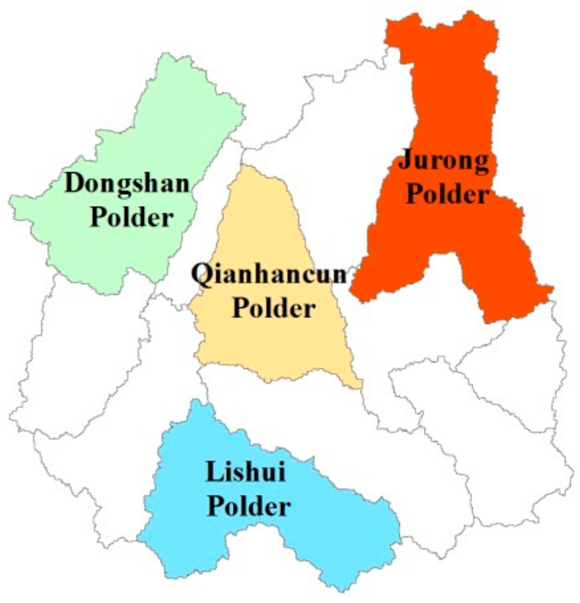
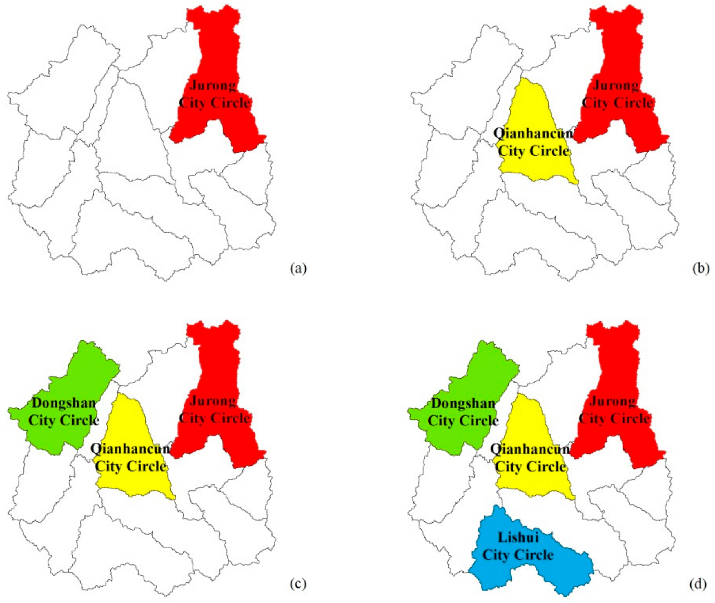
4.2. Impacts on Flood Risks of Polder Area

In order to study the impact of polder geographic distribution, four scenarios are examined, which are

(a)

Jurong City Circle only;

(b)

Jurong, Qianhancun City Circle combined;

(c)

Jurong, Qianhancun, Dongshan City Circle combined; and

(d)

Jurong, Qianshancun, Dongshan, Lishui City Circle combined.

From scenarios (a) to (d), the number and total area of polders increase (Figure 9).

Three rainfalls with different intensities were selected to analyze the flood risk for the four polder scenarios. The three rainfalls occurred on 3 August 1989 (light rainfall), 1 July 1987 (medium rainfall), and 30 June 1991 (heavy rainfall). The results are shown in

Table 6. The risk results of different polder distribution scenarios.

Flood No.	Scenario (a)				Scenario (b)
	Flood Volume (m3)	Peak Flow (m3/s)	Water Level (m)	Integrated Risk	Flood Volume (m3)	Peak Flow (m3/s)	Water Level (m)	Integrated Risk
1989	0.6636	0.8256	0.8077	0.6510	0.6796	0.8492	0.8140	0.6682
1987	0.8582	0.8372	0.8405	0.7934	0.8642	0.8449	0.8664	0.8102
1991	0.9603	0.9773	0.9731	0.9565	0.9644	0.9807	0.9828	0.9626
Flood No.	Scenario (c)				Scenario (d)
	Flood Volume (m3)	Peak Flow (m3/s)	Water Level (m)	Integrated Risk	Flood Volume (m3)	Peak Flow (m3/s)	Water Level (m)	Integrated Risk
1989	06990	0.8662	0.8652	0.6933	0.7140	0.8910	0.9515	0.7123
1987	0.8715	0.8579	0.8937	0.8290	0.8773	0.8743	0.9081	0.8446
1991	0.9632	0.9847	0.9838	0.9622	0.9645	0.9877	0.9937	0.9642

. The results show that flood risks increase as polder area and number increase. Integrated flood risk is smaller than marginal flood risks. For the minor flood in 1989, with the increasing polder area, the risk of flood volume and peak flow increase first, followed by increasing water level. For the medium flood in 1987, the risk increase of the water level was greater than that of flood peak. For the major flood in 1991, increasing polder areas had primarily influenced the water level and flood peak.

In general, polders in river basins increase various risk factors for basin-wide floods while protecting cities within the polders from flood. As polder area increases, the impact on flood risks escalates. For minor floods, flood risks are not high per se, and the impact due to polders does not appear to be a threat to the entire basin. A paradox is that increasing polder area will provide flood control to a higher area within the polder, but also cause increasing flood risks for the entire basin. Therefore, a tradeoff is warranted between protection for cities within polders and risk for the entire basin. To explore the tradeoff, polder failure is not considered here, that is, flood risk in the polder is zero. The product of the proportion of protected area in the basin and the integrated risks are used as a metric. The smaller the product, the better design of the polder. The results are shown in

Table 7. Reasonable analysis of different polder combinations.

Scenario	(1) Ratio of Area Protected by Polders	(2) Integrated Risk			(1) × (2)
		1989	1987	1991	1989	1987	1991
a	0.13	0.651	0.7934	0.9565	0.56	0.69	0.83
b	0.23	0.6682	0.8102	0.9626	0.52	0.63	0.74
c	0.34	0.6933	0.829	0.9622	0.46	0.55	0.64
d	0.45	0.7123	0.8446	0.9642	0.39	0.47	0.53

. Polder scenario (d) protects more urban areas and minimizes flood risks for the entire basin.

5. Conclusions

Based on the hydrologic and hydraulic simulations using HEC-HMS and HEC-RAS models for the Qinhuai River Basin, the Frank Copula flood risk model was developed to analyze flood risks in the basin for a range of scenarios. The following conclusions can be reached based on the results.

The exceedance probability of flood volume, flood peak and flood level for scenarios with polders is greater than that for scenarios without polders. The difference decreases as the return period increases. Polders increases flood risks for the area out of the polders. As flood magnitude increases, polders’ impact gradually decreases.

Based on the three-dimensional Copula risk model, the design values of flood volume, peak flow and flood level should be increased when polders are used. Under the present urban flood control standard, the flood control standard needs to be improved to protect the city in the polder when a polder is used.

When polders are used, the exceedance probabilities of flood peak and water level have a higher chance to exceed the design values determined in the Nanjing Urban Flood Control Plan. As flood magnitude increases, the impact of polders on flood risk levels off.

As the number and area of polders increase, flood risks also increase.

References

1. Luo, P.P.; Zhou, M.M.; Deng, H.Z.; Lyu, J.; Cao, W.Q.; Takara, K.; Nover, D.; Schladow, S.G. Impact of forest maintenance on water shortages: Hydrologic modeling and effects of climate change. Sci. Total Environ. 2018, 615, 1355–1363. [Google Scholar] [CrossRef] [PubMed]
2. Luo, P.P.; He, B.; Duan, W.; Takara, K.; Nover, D. Impact assessment of rainfall scenarios and land-use change on hydrologic response using synthetic Area IDF curves. J. Flood Risk Manag. 2018, 11, S84–S97. [Google Scholar] [CrossRef]
3. Luo, P.P.; Mu, D.R.; Xue, H.; Ngo-Duc, T.; Dang-Dinh, K.; Takara, K.; Nover, D.; Schladow, G. Flood inundation assessment for the Hanoi Central Area, Vietnam under historical and extreme rainfall conditions. Sci. Rep. Nat. 2018, 8, 12623. [Google Scholar] [CrossRef] [PubMed]
4. Jiao, T. Influence of construction in low-lying region on aquatic environment of city and countermeasures. Jiangsu Environ. Sci. Technol. 2006, S2, 121–123. [Google Scholar]
5. Luo, P.P.; He, B.; Takara, K.; Xiong, Y.E.; Nover, D.; Duan, W.L.; Fukushi, K. Historical assessment of Chinese and Janpanese flood management policies and implications for managing future floods. Environ. Sci. Policy 2015, 48, 265–277. [Google Scholar] [CrossRef]
6. Van Manen, S.E.; Brinkhuis, M. Quantitative flood risk assessment for Polders. Reliab. Eng. Syst. Saf. 2005, 90, 229–237. [Google Scholar] [CrossRef]
7. Gao, Y.Q.; Yuan, Y.; Wang, H.Z.; Schmidt, A.R.; Wang, K.X.; Ye, L. Examining the effects of urban agglomeration polders on flood events in Qinhuai River basin, China with HEC-HMS model. Water Sci. Technol. 2017, 75, 2130–2138. [Google Scholar] [CrossRef] [PubMed] [Green Version]
8. Gao, Y.Q.; Yuan, Y.; Wang, H.Z.; Zhang, Z.X.; Ye, L. Analysis of impacts of polders on flood processes in Qinhuai River Basin, China, using the HEC-RAS model. Water Sci. Technol. Water Supply 2018, 18, 1852–1860. [Google Scholar] [CrossRef]
9. Xing, W.B.; Xu, W.Y.; Wang, K.; Yan, X. Risk analysis of hydrological failures of levees in external Qinhuai River. J. Hohai Univ. Nat. Sci. 2006, 3, 262–266. [Google Scholar]
10. Xu, J.X.; Yao, S.P. A method to determine the mode of wipe off waterlogging on dyke. J. Agric. Mech. Res. 2008, 6, 61–63. [Google Scholar]
11. Zhao, G.F.; Jiang, Z.R.; Ding, Y.; Liang, G.Q. Assessment on risk analysis and risk evaluation of levees. China Water Transp. (Second Semimonthly) 2010, 11, 182–184. [Google Scholar]
12. Zhang, G.F. Polder construction and its ecological and social effects—An investigation of joint river embankment in Taihu Drainage Area (1950s–1970s). J. Minzu Univ. China (Philos. Soc. Sci. Edit.) 2012, 4, 36–41. [Google Scholar]
13. Xu, H.; Yang, S.J. Exploring the evolution of river networks in plain polders of Taihu Lake basin. Adv. Water Sci. 2013, 3, 366–371. [Google Scholar]
14. Yuan, Y.; Gao, Y.Q.; Wu, X. Flood simulation of flood control model for polder type based on HEC-HMS Hydrological Model in Qinhuai River Basin. J. China Three Gorges Univ. (Nat. Sci.) 2015, 5, 34–39. [Google Scholar]
15. Chen, H.R.; Wang, S.L.; Han, S.J. Assessment of field waterlogging risk in Lixiahe Plain Lake Region, Jiangsu Province: Case study from Yundong Plain in Gaoyou. J. Drain. Irrig. Mach. Eng. 2017, 10, 887–896. [Google Scholar]
16. Reddy, M.J.; Ganguli, P. Bivariate Flood Frequency Analysis of Upper Godavari River Flows Using Archimedean Copulas. Water Resour. Manag. 2012, 26, 3995–4018. [Google Scholar] [CrossRef]
17. Ganguli, P.; Reddy, M.J. Probabilistic assessment of flood risks using trivariate copulas. Theor. Appl. Climatol. 2013, 111, 341–360. [Google Scholar] [CrossRef]
18. Clayton, D.G. A model for association in bivariate life tables and its application in epidemiological studies of familial tendency in chronic disease incidence. Biometrika 1978, 65, 141–151. [Google Scholar] [CrossRef]
19. Frank, M.J. On the simultaneous associativity of F(x, y) and x + yF(x, y). Aequationes Math 1979, 19, 194–226. [Google Scholar] [CrossRef]
20. Genest, C. Frank’s family of bivariate distributions. Biometrika 1987, 74, 549–555. [Google Scholar] [CrossRef]
21. Chowdhary, H.; Escobar, L.A.; Singh, V.P. Identification of suitable copulas for bivariate frequency analysis of flood peak and flood volume data. Hydrol. Res. 2011, 42, 193. [Google Scholar] [CrossRef]
22. Genest, C.; Favre, A. Everything you always wanted to know about copula modeling but were afraid to ask. J. Hydrol. Eng. 2007, 12, 347–368. [Google Scholar] [CrossRef]
23. Klein, B.; Pahlow, M.; Hundecha, Y.; Schumann, A. Probability analysis of hydrological loads for the design of flood control systems using copulas. J. Hydrol. Eng. 2010, 15, 360–369. [Google Scholar] [CrossRef]
24. Fisher, N.I.; Switzer, P. Graphical assessment of dependence: Is a picture worth 100 tests? Am. Stat. 2001, 55, 233–239. [Google Scholar] [CrossRef]
25. Genest, C.; Boies, J.C. Detecting dependence with Kendall plots. Am. Stat. 2003, 57, 275–284. [Google Scholar] [CrossRef]
26. Burnham, K.P.; Anderson, D.R. Multimodel inference—Understanding AIC and BIC in model selection. Sociol. Methods Res. 2004, 22, 261–304. [Google Scholar] [CrossRef]
27. Suriya, S.; Mudgal, B.V. Impact of urbanization on flooding: The Thirusoolam sub watershed—A case study. J. Hydrol. 2012, 412, 210–219. [Google Scholar] [CrossRef]
28. Nanjing Urban Flood Control Planning Report. Available online: http://max.book118.com/html/2017/1105/139066558.shtm (accessed on 10 1 2018).
Figure 1. The location of the study area—the Qinhuai River Basin.
Water 10 01470 g001
Figure 2. The urban aggregation polders in the Qinhuai River Basin.
Water 10 01470 g002
Figure 3. Chi-plots and K-plots of pair-wise flood characteristics for scenarios with and without polders: (a) Graphical representation of strength of dependence using chi-plot (upper row) and K-plot (lower row), the pair-wise variables are V&P, V&Z and P&Z from left to right in order without UAPs; (b) graphical representation of strength of dependence using chi-plot (upper row) and K-plot (lower row), the pair-wise variables are V&P, V&Z and P&Z from left to right in order with UAPs.
Water 10 01470 g003
Figure 4. The correlation of empirical and theoretical frequency of marginal distribution: (a) The marginal fitting plots of the flood variables without UAPs; (b) the marginal fitting plots of the flood variables with UAPs.
Water 10 01470 g004
Figure 5. Two conditional probabilities of flood volume <300 m3: (a) ‘OR’ conditional probability of flood volume <300 m3; (b) ‘AND’ conditional probability of flood volume <300 m3.
Water 10 01470 g005
Figure 6. Two conditional probability contours of flood volume <300 m3: (a) ‘OR’ conditional probability contour of flood volume <300 m3; (b) ‘AND’ conditional probability contour of flood volume <300 m3.
Water 10 01470 g006
Figure 7. The exceedance probability curve of individual flood variables.
Water 10 01470 g007
Figure 8. Integrated flood risk comparison of Qinhuai River Basin with and without polders.
Water 10 01470 g008
Figure 9. The map of polder distribution: (a) Jurong City Circle only; (b) Jurong City Circle in the upper reach and Qianhancun City Circle in the middle reach; (c) Jurong City Circle in the upper reach, Qianhancun City Circle in the middle reach, and Dongshan City Circle in the lower reach; (d) Jurong and Lishui City Circle in the upper reach, Qianhancun City Circle in the middle reach, and Dongshan City Circle in the lower reach.
Water 10 01470 g009