Colloidal Crystallization in 2D for Short-Ranged Attractions: A Descriptive Overview

Abstract

With the aid of 2D computer simulations, the whole colloidal crystallization process for particles interacting with a short-ranged attractive potential is described, emphazising the visualization of the different subprocesses at the particle level. Starting with a supercooled homogeneous fluid, the system undergoes a metastable fluid-fluid phase separation. Afterwards, crystallite nucleation is observed and we describe the obtainment of the critical crystallite size and other relevant quantities for nucleation. After the crystal formation, we notice the shrinking and eventual disappearance of the smaller crystals, which are close to larger ones; a manifestation of Ostwald ripening. When two growing crystal grains impinge on each other, the formation of grain boundaries is found; it is appreciated how a grain boundary moves, back and forth, not only on a perpendicular direction to the boundary, but with a rotation and a deformation. Subsequently, after the healing of the two extremes of the boundary, the two grains end up as a single imperfect grain that contains a number of complex dislocations. If these dislocations are close to the boundary with the fluid, they leave the crystal to make it more perfect. Otherwise, they migrate randomly inside the grain until they get close enough to the boundary to leave the grain. This last process of healing, trapping and getting rid of complex dislocations occurs preferentially for low-angle grain boundaries. If the angle between the symmetry axes of the two grains is not low, we end up with a polycrystal made of several touching crystal grains.

1. Introduction

There is an ongoing interest in crystals made of colloidal particles [1,2]. One of the reasons for this is the possibility to adjust the interaction potential between the particles by chemically modifying their surfaces, which would allow us to study the many different structures obtained by self-assembly. Another important reason is the capability of researchers to study the crystallization process by direct observation with simple laser diffraction and optical video microscopy, given that their size and interparticle distance is usually comparable to the wavelength of visible light and that their dynamics is slow enough to follow the trajectories of the individual particles [3,4,5,6,7]. Last but not least in importance is the possibility of applying some of the colloidal crystalization results to the self-assembly of proteins in their native globular state, a topic with the utmost attention paid in recent years; although in this case, by their very nature, the interaction between the proteins is not isotropic as with spherical colloidal particles, which enriches but complicates the problem [8].

In particular, the monolayers of colloidal particles trapped by surface tension on the free surface of a liquid have been proposed as two-dimensional (2D) analogs of 2D atomic systems in the condensed phase. P. Pieranski was the first to observe the formation of a 2D colloidal crystal, made of polystyrene spheres confined in a surface energy well at the air-water interface [9]. Using particles of a diameter ≃ 0.2 $\mathsf{\mu }$m in a low-ionic-strength aqueous medium, he observed that ordering occurs with particles separated from each other by distances of at least ten particle diameters. Since in this case only a part of the surface of the colloidal spheres is immersed in water, allowing dissociation of the sulfonic acid groups on that part of the surface, the ordering was attributed to the repulsion of electric dipoles perpendicular to the air-water interface, formed at each particle due to the asymmetric distribution of such dissociated charges [9].

A distinction must be made between this process and that of crystallization of usual atomic systems, for which the attractive interaction potential is somewhat similar to that of a Lennard-Jones 6–12 type. In the present case, due to a fixed concentration, the system may crystallize with purely repulsive forces in order to minimize its free energy, if the concentration is high enough. This has been seen since the earlier studies of the crystallization of a 2D electron gas on a liquid-He surface [10]. A necessary condition therefore is that the repulsive interaction range should be longer than the nearest-neighbor distance between the particles; for low enough concentrations, crystallization may not occur. For dilute systems, an attractive interaction potential is required to order the system into a crystal. Onoda [11] was the first to succeed in finding the correct particles in this other case. They consisted of large uniform polystyrene particles of different sizes (from 1 to $15\mathsf{\mu }$m), stabilized with the surfactant sodium dodecyl sulfate on their surfaces, to prevent the aggregation of the particles. The attractive interaction potential was coming therefore from the van der Waals forces experienced by two nearby particles plus the hard core at contact. He found clustering and ordering of the system, resembling in the first steps a phenomenom similar to crystalline nucleation [11].

Another distinction should be made between the process we are describing and that of melting and crystallization of 2D systems when they are kept in thermal equilibrium, that is, if the heating (cooling) rate for melting (crystallization) is made to be very slow. In this last case the situation is not quite clear since, with the exception of some studies (e.g., [12,13,14,15]) that find a first order transition from the liquid to the solid or vice versa, most researchers find two phase transitions with a hexatic phase in between the fluid and the crystal phases. However, some of them find the two transitions to be continuous [16,17,18,19,20,21], while some others [22,23,24,25,26] find one or the two transitions to be first order (indicating a coexistence of the phases at the transition point), depending on the repulsive interaction potential. The two continuous phase transitions scenario was predicted by the celebrated KTHNY theory, after Kosterlitz and Thouless [27], Halperin and Nelson [28], and Young [29]. As colloids can be easily visualized by video microscopy, this prediction has been verified in such 2D colloidal systems [16,17,19,20,21], finding no hysteresis of the transition points in melting and cooling cycles of the system, if it is kept always in thermal equilibrium. In the case described here the 2D system, initially at a high temperature, is suddenly quenched to a supercooled state and it is not in equilibrium. The crystallization process is the result of the system trying to reach the equilibrium state. In this case it has been shown [30], at least for super-paramagnetic colloids in water with repulsive dipole-dipole interactions, that the system crystallizes from the isotropic fluid directly to the crystal, without any intervening hexatic phase.

In a supercooled homogeneous fluid, it is generally believed that crystallization first begins with the formation of small crystalline regions, called crystalline nuclei or simply crystallites, most of them disappearing almost immediately after formation while a few of them, with a extent larger than a critical size, continue to grow to form a crystal grain. It turns out that for some colloidal particles with short-ranged attractive interactions in 3D [31,32,33,34] and 2D [35,36,37], and also for some colloidal-like particles again with short-ranged attractive interactions, notably the proteins [38,39,40,41,42], this paradigm may not be true. In the usual crystallization of atoms or small molecules, the range of the attractive interactions is generally of the same order of magnitude as the size of such atoms, as in a Lennard-Jones potential. However, in mixtures of depletants (such as polymers) and colloidal particles, where the length of the polymers is chosen such that their radius of gyration is sufficiently small compared to the diameter of the colloids, the colloidal particles are attracted to each other by means of a short-ranged depletion interaction [43]. Similarly, for many purposes, globular proteins are well described as hard spheres with short-ranged attractive interactions [44]. In all these cases, the single phase colloidal fluid does not nucleate directly to the crystal phase. It happens that an intermediate, metastable fluid-fluid phase separation occurs first [31,32,33,34,35,36,37,38,39,40,41,42]. Afterwards, crystal nucleation occurs in the denser portions of the phase separated colloidal liquid.

Most of the theories of crystallization consider the boundaries between the crystallites or the crystals and the surrounding fluid as smooth. In fact, in the classical nucleation theory [45], the crystallites are assumed to have a spherical shape (circular in our 2D case). The growing of these regions into a crystal depends upon two factors: a decrease in the bulk energy which favors growth, and an increase in the surface energy which disfavors it. These factors are reflected in the free energy change for the formation of a circular crystallite (in 2D) of radius r:

$$\Delta G=2\pi r\gamma -\pi r^2\Delta \mu n$$

(1)

where γ is the line tension of the crystallite boundary with the fluid, $\Delta \mu ={\mu }_{fluid}-{\mu }_{crystal}$ is the difference between the chemical potentials of the fluid and crystal phases and n is the number of particles in the crystal per unit area. This free energy difference has the form of a barrier and is sketched in Figure 1, where the critical crystallite radius is given by

$$r_c=\gamma /n\Delta \mu$$

(2)

As it is somewhat difficult to calculate γ and $\Delta \mu$ from first principles they are, more often than not, treated as parameters adjusted to fit the experiments. Notwithstanding the assumption of smooth surfaces for the crystallites and crystals made in the classical nucleation theory, a considerable amount of researchers are finding rough interfaces, at least for colloidal crystals. For example, in the 3D experimental work of Gasser et al. [46] it was shown by confocal microscopy the anisotropy and the rough surface structure of colloidal crystalline nuclei and crystal grains. It was also shown how to calculate the critical crystallite size from a knowledge of the position of the particles during the course of the time. However, for calculating the interfacial tension and the chemical potential difference between the phases, to take into account their anisotropy the authors approximated the crystallites and crystals as ellipsoids which, after all, have smooth surfaces. Moreover, it has also been shown [47] that the crystallization front of a growing complex plasma crystal is not only rough, but it has a fractal (scale invariant) structure. It appears that more and more researchers are finding anisotropic crystallites with rough surfaces [48,49], suggesting that more advanced nucleation theories must be developed that can treat the nucleus structure as a variable.

Once some of the crystallites surpass the critical size they keep growing, acquiring more particles from the surrounding liquid that attach to their boundaries. In this sense, the crystal boundaries are not static but highly dynamical, collecting and releasing particles from and to the surroundings. It is remarkably found an interchange of particles between two nearby crystal grains through the surrounding liquid leading, in some cases, to the shrinking and eventual disappearing of the smaller of the two “interacting” grains. This result is due to the higher stability of the larger grains as described in Equation (1) and Figure 1: The larger crystals have a lower curvature of their boundaries and a (negatively) large bulk free energy, which favors their growth. The smaller crystals on the other hand account for a higher boundary energy per unit area and are “devoured” by the larger crystals. This process, known as Ostwald ripening, was first described by Wilhelm Ostwald more than a century ago [50], in which the components of a discontinuous phase (not necessarily crystalline) preferentially diffuse from smaller to larger droplets through the continuous phase, and has been verified in many instances of crystalline droplets [51,52,53,54].

At some point, depending on the concentration of the particles [55], the crystals start to touch each other [30] which imposes the formation of the grain boundaries (GB); in the course of time, the crystalline system becomes a cellular structure [56] whose “cells” are the so called crystal grains. Afterwards, the process of grain coarsening switches from the simple growth of the crystal acquiring particles from the surrounding fluid to the coarsening arising from the movement and migration of the GBs, which forces the small grains to shrink and disappear while the large ones grow at their expenses. But it is also possible (as we will see) the disappearance of the GB between two crystals, that therefore coalesce into a single, larger crystal. Due to the misorientation of the symmetry axes of the two impinging monocrystals, they do not merge immediately into a single crystal. This merging may occur, after some time, if the following conditions are satisfied: (i) the touching crystals are not too large; and (ii) the misorientation angle of the symmetry axes of the crystals is also not too large. Before this merging, GB diffusion and migration takes place [57], particularly faster in the low misorientation angle cases in 2D [58]. At the particle level, it was observed a glassy type dynamics of the particles confined in the grain boundaries, due to transient caging of them by their nearest neighbors [59,60]. It has been seen, both by simulations [61] and experiments [62], how a grain boundary diffuses back and forth on a direction roughly perpendicular to the boundary, as if performing a one-dimensional random walk, although it was observed for short periods of time.

If the misorientation angle is low, the grain boundary is named low-angle grain boundary (LAGB), while if it is high it is termed high-angle grain boundary (HAGB). The transition angle from LAGBs to HAGBs is around 10${}^{\circ }$–15${}^{\circ }$ [57,63], but depends on the material and boundary structure. In the case of HAGBs, the crystallizing system may remain as a polycrystal for a long time, which is the case of most metals found in nature. In the other case of a LAGB, as mentioned, the two touching crystals may merge into a single crystal with the disappearance of the grain boundary. Once the LAGBs in the system have disappeared through this process, the final product of the crystallizing system is obtained, the polycrystal, formed by grains separated by HAGBs.

The purpose of the present article is to describe all these mentioned subprocesses, present in the crystallization of colloidal particles interacting with short-ranged attractive interactions, which are many times dispersed in the literature, and try to unify them into a single entity for the whole colloidal crystallization process. The description of the processes at the particle level will be illustrated with figures and videos taken from Monte Carlo simulations designed to exhibit the crystallization of colloidal particles in 2D interacting with the aforementioned potential. It will be seen how the simulations reproduce most of the processes and, more remarkably, they produce some others not yet described that need further explanation.

2. Simulations

Considering that the crystallizing units are mesoscopic colloids suspended in a fluid, and considering also that we are interested in the time evolution of the crystallites and crystals, the ad hoc simulation procedure should be either a Brownian dynamics simulation or a kinetic Monte Carlo simulation with short random steps, since the colloidal particles are performing that kind of diffusional motion. Although kinetic Monte Carlo, which is just a way of solving the master equation, should be complemented with the approximate transition probabilities from one state to the next, Kikuchi et al. have shown [64,65,66] that by using a Metropolis dynamics [67] they can recover the Fokker-Planck diffusion equation. The only restriction imposed in their derivation is that the maximum allowed displacements of a particle should be sufficiently small compared to the size of the system and to the irregularities of the potential between the particles [66]. Therefore, a kinetic Monte Carlo simulation with Metropolis dynamics is equivalent to a Brownian dynamics simulation.

We considered $N_{tot}=53,715$ monodispersed disks distributed at random in a box with periodic boundary conditions, taking care not to overlap the hard cores. The hard cores occupy an area fraction of $\varphi =0.15$. Our system size is sufficiently large and the area fraction sufficiently small that finite size effects can be neglected during the course of crystal nucleation [68]. In crystal nucleation simulations, it seems that a great deal of uncertainty rests on the definition of the crystallites [69]. In the case of attractive interactions, this is probably due to the broad potential wells mostly used, like the 6–12 Lennard-Jones potential for which the width of the attractive well is of the same order of magnitude as the size of the repulsive core. The reason of our use of a narrow potential well is therefore twofold: (i) As it will be seen, the crystallites obtained could be very easily defined with almost no ambiguity; and (ii) it will be possible to retrieve the metastable fluid-fluid phase separation that occurs before the crystal nucleation, when the particles are interacting with a short-ranged potential. The crystal nucleation will be obtained afterwards in the denser portions of the phase separated system, We experimented with different continuous potentials with narrow wells, which would define with more precision the separation of two bonded particles, until we settled with the one shown in Figure 2, whose mathematical expression is as follows: $V/k_{B}T=(75/r^3)exp(-2.5(r-1))cos\left(10{(r-1)}^4\right),$ where r is the distance between the particles normalized by the hard core diameter. After the cosine reaches zero for a second time, at around $r_0\simeq 1.8285$, the potential is made to be zero. This potential was tabulated to speed up the calculations. The algorithm is as follows: (i) pick one particle at random and move it by a distance equal to one tenth of the hard core diameter on a random direction; (ii) Calculate the new energy of interaction $U_f$ and substract from it the initial: $\Delta U=U_f-U_i$; (iii) If $\Delta U\le 0$ the move is accepted; (iv) If $\Delta U>0$ the move is only accepted if $exp(-\Delta U/k_{B}T)>R$, where R is a random number uniformly distributed in [0, 1); (v) After each trial move, whether or not it is accepted, the Monte Carlo time t is augmented by $1/N_{tot}$. We then go to point (i). When $\Delta t=1$, which defines a Monte Carlo sweep, every particle has attempted to move once, on average. From now on, when we refer to the Monte Carlo time (MC time), we will mean the Monte Carlo sweeping time. The simulations were stopped at the MC sweeping time of 128,000, after waiting several months of wall-clock time.

3. Description of the Subprocesses

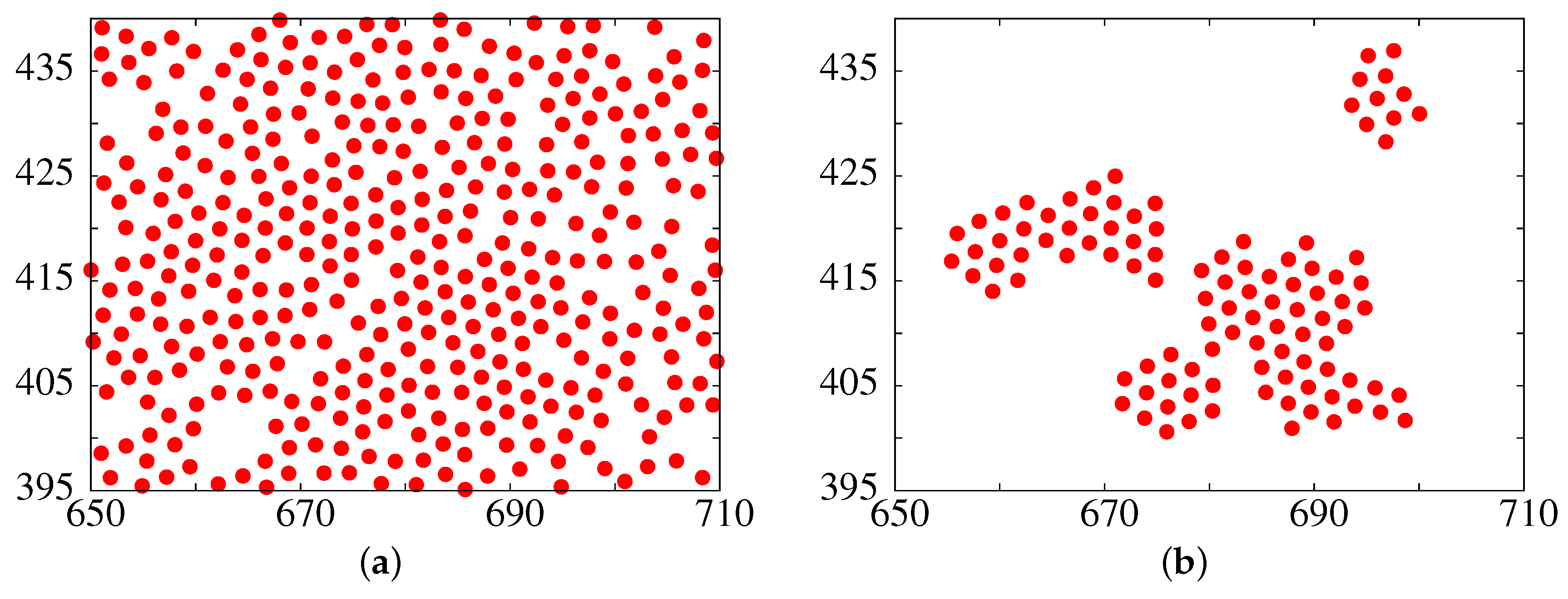
3.1. The Metastable Fluid-Fluid Phase Separation

As already mentioned, in systems with short-ranged attractions between the particles, it has been found in 3D [31,32,33,34,38,39,40,41,42] and 2D [35,36,37] that crystal nucleation does not start from the homogeneous supercooled system of particles. It turns out that a fluid-fluid phase separation occurs first (now called two-step nucleation in the literature); the crystalline nuclei, particularly those of a larger size, appear in the denser portions of the fluid-fluid phase separated system. In the case under study here, it was also seen [70] that the larger crystallites appear in the denser portions of the phase separated system. A few of those crystalltes, when they surpass the critical size, continue their growth to become part of the final crystalline phase. This is schematically shown in Figure 3, where we can see a metastable fluid-fluid coexistence (indicated by the dashed curved) which lies inside the final fluid-crystal coexistence curve. After thermalizing the system at high temperatures for 2000 MC sweeps, that is with a potential strictly equal to zero after the hard core, we started to count the MC time using the potential shown in Figure 2. This corresponds to the sudden quench to the supercooled state already mentioned. In Figure 4a it is shown the state of the system at the beginning of the process, at $t=1$, i.e., after one Monte carlo sweep. By zooming in the figure with the computer viewer, we are able to see a quite homogeneous system even at the particle level. On the contrary, in Figure 4b for the MC time t = 4001, it is seen high density regions coexisting with low density regions, both disordered.

A convenient measure of the crystallinity for the overall 2D system is given by the global bond orientational (hexagonal) order parameter ${\psi }_6$, first introduced by Halperin and Nelson [28,71] in the context of two-dimensional melting. The local value of ${\psi }_6$ for a particle j located at ${\mathbf{r}}_j=(x,y)$ is given by

$${\psi }_{6,j}=\frac{1}{N_j}\sum _{k}exp\left(6i{\theta }_{jk}\right)$$

(3)

where the sum on k runs over the $N_j$ nearest-neighbors of this particle, and ${\theta }_{jk}$ is the angle between the line joining the particles j and k and an arbitrary but fixed reference axis, e.g., the x axis. The nearest-neighbors are obtained via the Voronoi/Delaunay construction (For a definition of the Voronoi cell around one of our disks and the overall Voronoi tesselation, see [72]). The global bond orientational order parameter is then defined as [73,74,75]

$${\psi }_6=\left|\frac{1}{N_{tot}}\sum _{j=1}^{N_{tot}}{\psi }_{6,j}\right|$$

(4)

when the system belongs to the fluid phase and there is no structural order, its value is ${\psi }_6\ll 1$. On the other hand, ${\psi }_6$ takes a value very close to (but smaller than) unity when the colloidal particles form a monocrystal with the hexagonal order (triangular lattice).

In Figure 5 it is plotted ${\psi }_6$ as a function of the MC time. For the time $t=1$ the value of ${\psi }_6$ is so low that does not appear in the graph. For the time t = 4001, its value is ${\psi }_6=0.001458$, which is still very low and corroborates the assertion that at this time, for the system considered here, the two coexisting fluid phases are both disordered. It was found in our system [70] that the nucleation process starts around $t\approx$ 4500, in the sense that it is possible to find crystallites with the symmetry of the triangular lattice containing more than, say, ten particles. Before this time, for example at t = 4001 of Figure 4b, only crystallites with less than ten particles were found. The crystallites were forming mainly (if not entirely) in the denser portions of the fluid-fluid phase separated system, indicating therefore supersaturated zones. That the ${\psi }_6$ does not reach the monocrystal value of one in Figure 5 is due to the orientational mismatches between the different grains. The limiting value found at long times for ${\psi }_6$ (see Figure 5), of around 0.2, lies in the range of values found for some other 2D polycrystalline systems made of colloidal particles [76].

Two comments are in order at this point. First, it should be emphasized that the process considered here is homogeneous nucleation, which occurs by the spontaneous formation of a critical nucleus in the bulk of a supercooled fluid. This is generally a very rare event, since it happens due to random structural fluctuations [2]. Researchers need to wait for quite a long time, both experimentally or with simulations, to sometimes observe the appearance of a critical nucleus in homogeneous nucleation. In heterogeneous nucleation, on the other hand, the formation of a critical nucleus on an already present seed (e.g., an impurity) can be much faster, if the seed gives rise to a reduction of the free energy barrier (see Figure 1). To have a colloidal crystal with an increased purity, homogeneous nucleation should be used. What is then needed is an enhancement of the crystal nucleation rate by many orders of magnitude, in order to efficiently produce the crystals. It has been proposed, both by simulations [39] and Density Functional Theory [40], that such an enhancement can be promoted by nucleating the system close to the the metastable fluid-fluid critical point, which reduces the free energy barrier. However, it could be a nuisance to find the metastable critical point in order accelerate the crystal nucleation. Nonetheless, recent work on Density Functional Theory has shown that this is not necessary. Lutsko and Nicolis [77] have found that by just supercooling inside the fluid-fluid coexistence, it is free-energetically easier to crystallize by passing through a metastable dense fluid. This agrees with the study of Galkin and Vekilov [41] for protein crystallization around the liquid-liquid phase boundary. This also agrees with the observation here that the crystalline nuclei, in particular the larger ones, appear precisely at the denser portions of the fluid-fluid phase separated system. In other words, an already supercooled system may be made highly supersaturated and prone to crystallize by an increase in its density. A thorough resolution of this still unsolved issue is very relevant, and of particular importance, to the protein crystallization process.

Second, we were expecting to witness [70] a full fluid-fluid (or liquid-gas) phase separation, perhaps with droplets of the denser disordered phase inside the dilute one, also disordered [42], before the system started to crystallize. Instead, as already mentioned, the crystal nucleation started to take place at the time $t\approx$ 4500, for which there were only high density regions (far from being circular) coexisting with low density ones, as in Figure 4b. This revealed us (and we realized) the meaning of what a metastable state is: Soon after the formation of the dense and dilute regions, the crystal nucleation process started to take over, benefitting from the higher concentration of particles in the denser regions, without having to wait for the formation of droplets of any given shape. This is probably due to a not-so-high value for the free energy barrier in the nucleation process (see below). Therefore, it is quite possible—for some other conditions of the system—to have a more established fluid-fluid phase separation, before the crystal nucleation process starts.

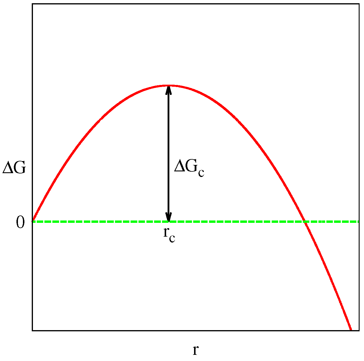
3.2. Crystalline Nucleation

By visualizing the simulations results, it was possible to see after the time $t\approx$ 4500 the continuous formation and disappearance of small and medium sized crystallites, the larger ones being formed at the denser zones of the fluid-fluid phase separated system. Only a few of the larger ones could be able to surpass a critical size and started to grow steadily. As highly anisotropic crystallites were observed with rough (possibly fractal) boundaries, as the ones obtained in the experimental work of Onoda [11], the critical size was obtained not in terms of any critical radius but in terms of the critical number of particles, $N_c$. Movies, at the particle level, were produced from the simulations to investigate the path to the formation of supercritical nuclei and to ascertain which are the main working mechanisms in this process. They were also produced to observe the growth of the crystals, above the critical size. In video 1, that lasts 3 min 20 s, we investigate the appearance of a supercritical nucleus, by focusing in one of the dense regions of the simulation box. As mentioned, it can be observed the incessant generation and vanishing of small and medium sized crystallites, with a triangular lattice symmetry, coming from the structural fluctuations of the system. The critical size was estimated [70] at $N_c\approx 75$ (see below), and most of the crystallites studied coming from those structural fluctuations were well below that size. One possibility to obtain a crystallite with a supercritical size comes from the merging or coalescence of two nearby subcritical size crystallites, such that the symmetry axes of them more or less coincide, i.e., with a low misorientation angle. Indeed, this is seen in video 1 at the time 1 min 17 s in supplementary materials, when a merging of two crystallites is observed. After this merging and some restructuring of the resulting crystallite, it was observed a steady growth of the crystal, which indicated that it surpassed the critical size. Although we do not discard a large structural fluctuation beyond the critical size as the path to the formation of a supercritical size crystallite, it was found an easier way to obtain such a large crystallite. This coalescence of subcritical crystalline nuclei to obtain a supercritical one has been also observed experimentally in reference [36].

For the analysis of the nucleation and crystallization processes, a program was designed to isolate crystallites and crystals with more than 10 particles (there are an enormous quantity of smaller crystallites, which would be hopeless to analize). Two bonded particles belonging to a crystallite or to a crystal are located, on average, at a distance equal to the minimum of the potential well. Nonetheless, as the particles are vibrating around this minimum, we considered them to be bonded if their separation is less than $r_0$, the distance after which the interaction potential is zero. In this 2D case, the criteria for considering a particle to be “crystal-like” is that it should have at least two bonds with other particles in the same crystallite or crystal, since if it has only one bond, it can swivel on the plane until it gets “hooked” by another particle and becomes part of the crystallite or crystal, or the bond is broken by a thermal fluctuation and the particle diffuses away. The tolerancy for the angle between any two adjacent bonds in the crystals emanating from a particle was taken as ${12}^{\circ }$, from the expected ${60}^{\circ },{120}^{\circ }$ or ${180}^{\circ }$ values. This ${12}^{\circ }$ value was defined for our potential by observing that the crystallites obtained by increasing this tolerancy by about 100% were essentially the same. If we had put a $6^{\circ }$ value, for example, for this tolerancy and, by increasing it again by 100%, the crystallites obtained would have been rather different, with substantially more particles in each crystallite. However, experimenting with narrower potential wells, we have seen that the tolerancy could be made smaller.

To appreciate the goodness of the algorithm, in Figure 6 it is presented the extraction of crystallites and crystals with more than 10 particles. As can be seen, the crystallites shown have a distinct triangular lattice symmetry. The program was able to proportion the number of particles of each crystallite or crystal, N, its radius of gyration, $R_g$, and the number of particles in its “outer” boundary, L. That is, excluding the particles surrounding a vacancy, unless they also belong to the outer boundary.

To obtain the critical crystallite size with the method of Gasser et al. [46], the growing or shrinking of those crystallites were followed during the course of the simulation, from one frame to the next after a Monte carlo sweep. This was performed with another algorithm. It allowed the calculation of the probabilities of growing ($P_g$) or shrinking ($P_s$), averaged inside intervals of constant magnitude in the logarithmic size scale N [70]. The quantity $P_g$ – $P_s$ should be negative for small sizes and positive for supercritical sizes [46]. Therefore, the point at which this function crosses zero marks the critical size. In this way, the critical size for our system was estimated between 70 and 80 particles [70].

In Figure 7 is shown an example of a critical size crystallite. As it is evident from the figure, the boundary of the crystallite is still rough (possibly fractal). The fractality [78] of the crystallites and crystals was investigated. It was found that the crystallites and crystals carried—in a statistical sense—both a mass (or bulk) fractality with a fractal dimension denoted as $D_f$, and a boundary fractality with a fractal dimension named $d_f$. To obtain the mass fractality, a double-logarithmic plot was made of the radius of gyration versus size, N, of all the crystallites and crystals studied (above 10 particles), averaged again inside intervals of constant magnitude in the logarithmic size scale. This is a standard way for calculating the fractal dimension of colloidal aggregates, particularly when studying not only large but also small clusters, for which a box counting procedure cannot be performed (see for example, [79]). Surprisingly, it was found the apparition of not one but two straight lines with the breaking point at precisely around the critical crystallite size. From the plot, the bulk fractal dimension of the crystallites was derived as $D_{f1}=1.873\pm 0.059$ while that for the crystals was obtained as $D_{f2}=2.059\pm 0.134$, where the error bars correspond to twice the standard deviation and give a 95% confidence on the results. Since, on physical grounds, $D_f$ cannot be greater than 2 for a 2D system, the bulk fractal dimension of the crystals was taken as exactly 2, a value which lies well inside the interval for the $D_{f2}$ found. Therefore, the crystals are compact. However, for the crystallites it was found a value which is definitely smaller than 2, indicating that they are fractal in a statistical sense. As can be seen in Figure 8a, sometimes the crystallites have a chainy structure, resembling the diffusion-limited colloidal aggregation (DLCA) clusters [80], although not as stringy as the DLCA aggregates. On top of that, many other crystallites are not chainy but bulkier (see e.g., Figure 6). These two facts increase their fractal dimension from the DLCA value (≃1.45) to the value just found. Note how this value of the fractal dimension compares rather well to the value of 1.8 reported by Dillman et al. [76]. However, above the critical size, the crystals are compact in the interior, which gives a bulk fractal dimension of around two, as Figure 8b shows. To obtain the boundary fractal dimensions, several procedures were used, all giving the same results. In one of them it was plotted double-logarithmically the number of particles in the outer boundary, L, versus a linear dimensions of the cluster, which could be taken as the radius of gyration. This is similar to the procedure used for calculating the $d_f$ of the Koch’s curve [78]. In this way it was obtained $d_f=1.318\pm 0.065$ for the crystallites and $d_f=1.168\pm 0.071$ for the crystals. This indicates that the crystallites have a rougher boundary compared to a more rounded boundary of the crystals, which is evident when comparing Figure 6b, Figure 7b and Figure 8b. No claim on the universality of these four fractal dimensions was made. They may vary with a change in the interaction potential, the degree of supercooling, and even with a change in the concentration.

It was intriguing to observe that the critical crystallite size, obtained by the probability method, roughly coincided with the breaking points of the straight lines in the fractal analysis of the crystallites and crystals. In video 1 we can see that the crystallites are very fleeting and ephemeral, for which we can only have a glimpse of them. They may grow by acquiring some more particles from the surrounding fluid, that attach to their boundaries or, much more often than not, they can shrink by losing particles from their boundaries and, afterwards, disappearing. However, in the last part of this video and in video 2, we can see that when the crystallites reach an appreciable size (greater than the critical size), they become more or less permanent. Nonetheless, the boundaries are not fixed but very active, acquiring more particles from the surrounding fluid, that eventually go into the cavities of these boundaries rather than at their tips, in order to establish more bonds with other particles of the structure and “feel more comfortables” with a lower energy. This selection of the attaching sites cannot be obtained from the crystallites because, during the time interval for which a particle of the surrounding fluid tries to do so, the crystallite disappears. The net effect of these processes is that, for the crystallites, the boundaries stay approximately as they were formed, having a rough structure, while, for the crystals, a smoother boundary results from the filling of their cavities by the particles of the surrounding fluid. Therefore, the transition from ephemeral crystallites to perdurable crystals marks also the transition from a relatively high boundary fractal dimension to a low boundary fractal dimension.

Instead of the classical free energy of formation of a circular crystallite of radius r (see Equation (1)), it was written explicitly in terms of the length of the boundary $l=L{l}_o$, where $l_o$ is the lattice spacing (which corresponds to the position of the minimum of the potential well), as well as the number of particles N:

$$\Delta G=\gamma l-\Delta \mu N$$

(5)

As is well known, the first term $\gamma l$ dominates this change for the small crystallites. The probability of activation of a crystallite of size N and boundary l scales as $exp(-\beta \Delta G).$ Therefore, the number of small crystallites in the system scales as $NCr\sim exp(-\beta \gamma l)$. A logarithmic plot of $\left(NCr\right)$ versus L was made [70], for which a very good straight line was obtained for the first 10 points in the graph, from $L=10$ to $L=20$. From that plot the line tension of the crystallites was obtained as

$$\gamma \simeq 0.399k_{B}T/l_o$$

(6)

From the fractal analysis just mentioned it was possible to get a relationship between the boundary size (L) of the crystallites and crystals and the number of particles in them (N). This equation reads:

$$L=2.502N^{0.631}$$

(7)

Next, Equations (6) and (7) were substituted into Equation (5). Then the derivative with respect to N was equated to zero at $N=N_c\simeq 74$, say, to obtain $\Delta \mu \simeq 0.128k_{B}T$. With all these values, the height of the free energy barrier was calculated as [70]:

$$\frac{{(\Delta G)}_c}{k_{B}T}\simeq 5.58$$

(8)

This barrier is not so high to be unsurmountable by a free energy fluctuation. Unfortunately, to the best of our knowledge, there are not 2D experimental results to compare with Equations (6)–(8).

A comment should be said at this point. The reason that most (if not all) of the medium and large size crystallites were coming from the high density zones of the fluid-fluid phase separation is that, for a short-ranged interaction, the particles in those zones were quite close to each other and the bonds, as defined above, were not very difficult to form. The only remaining thing to produce a crystallite is a thermal fluctuation that could orient those particles to arrange with a triangular lattice symmetry. Therefore, the line tension and the chemical potential difference should refer to this zone. In other words the line tension γ is between the crystallites or crystals and the high density zone of the fluid, at least for the initial stages of the nucleation process. Moreover, there should be (at least) 3 chemical potentials: one for the low density zone of the fluid, another for the high density zone, and additionally another one for the crystalline phase. Therefore, the $\Delta \mu$ should refer to the difference between the chemical potentials of the high density fluid and the crystalline phase, again at least for the initial stages of the nucleation process. Nonetheless, as time proceeds, the supercritical crystals keep growing and reach a linear size comparable to the size of the high density zones of the system, which can be considered of the order of the correlation length of the particles inside the fluid-fluid phase separation. Afterwards, the crystals in their growth become in contact with the low-density zones, which can be called the gas phase. The subsequent growth comes from the crystals acquiring particles from this gas phase, a process that could be called desublimation. But it should be stressed that the nucleation process occurs in the denser (liquid) zones of the fluid-fluid phase separation.

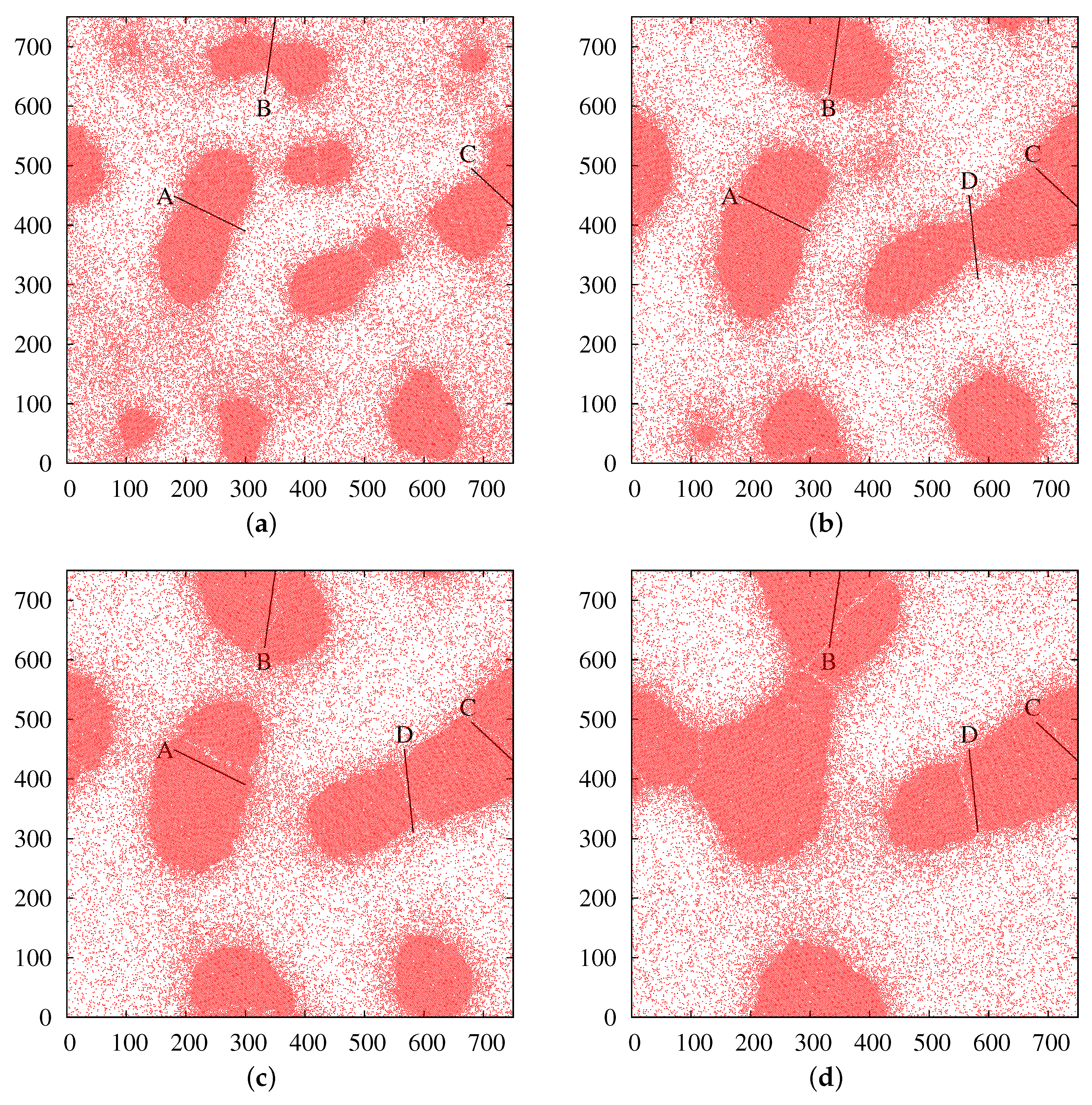
3.3. Ostwald Ripening

For an usual experimental or simulational system with a constant number of colloidal particles in a fixed space (a square box of area A in our case), and due to the fact that the density in the crystals is higher than in the fluid (at least for potentials with an attractive well as in our case), as the crystallization proceeds the fluid becomes less and less dense. This, in turn, forces the fluid chemical potential to diminish, making the $\Delta \mu$ in Equation (2) to diminish also. Therefore, the critical radius keeps increasing. Hence, some of the formerly supercritical crystals become subcritical and prone to shrink and disappear. It sometimes happens that when two nearby crystals with dissimilar sizes, “interacting” by an interchange of particles between them, it occurs that the particles diffuse preferentially from the smaller to the larger crystal, due to the lower boundary energy per unit length (in our 2D case) of the larger crystal.

As already mentioned in the introduction, this is referred to as Ostwald ripening [50,51,52,53,54]. In Figure 9 this phenomenon is illustrated where, on the left, we can see two nearby crystals “interacting” through a cloud of particles at the MC time of 21,001 while, on the right for the MC time of 35,001, the smaller of the two crystals has almost disappeared, leaving a cloud of particles as the only vestige of its existence. The same phenomenon was observed at several other sections of the lattice in our simulations. All this may suggest that, if instead of working in the canonical ensemble (at fixed $N_{tot}$, T and A), we would be working in the grand canonical ensemble by placing an open system in contact with a reservoir of particles at fixed chemical potential μ (the so-called $\mu TA$ ensemble), we would not obtain Ostwald ripening, something that must be confirmed.

The theoretical work on Ostwald ripening and the subsequent grow of separated (non-touching) crystals is mostly based on the fundamental work done by Lifshitz and Slyozov [81] and independently by Wagner [82], the LSW theory. The coarsening of the crystals occurs in order to reduce the boundary free energy with respect to the surrounding solution. It is a direct consequence of the Gibbs-Thomson equation that describes the dependency of crystal solubility on crystal grain size [83,84,85,86,87]. For our 2D case, this equation reads:

$$C\left(r\right)=C(\infty )exp(\alpha /r)$$

(9)

where $C\left(r\right)$ is the solubility of a dispersed phase crystal with radius r, while $C(\infty )$ is the bulk solubility, that is, the solubility of a crystal with infinite radius, corresponding to the concentration of the fluid particles in equilibrium with the crystal phase. α is the so called capillary length given by

$$\alpha =\frac{k_l\gamma }{2k_{a}n{k}_{B}T}$$

(10)

where $k_l$ and $k_a$ are the boundary-length and area shape factors ($k_l=2\pi$ and $k_a=\pi$ for a perfect circle). γ is the line tension of the crystal boundary, n is the number of particles per unit area inside the crystalline phase and $k_B$ is Boltzman constant. Equation (9) is just another instance of Equation (2) and can be derived from it. For a perfect circle $r_c=\gamma /n(\mu \left(C\left(r_c\right)\right)-{\mu }_{cryst})$ and, by its own definition, ${\mu }_{cryst}=\mu \left(C(\infty )\right)$ by the condition of phase equilibria. Therefore $r_c=\gamma /n(\mu \left(C\left(r_c\right)\right)-\mu \left(C(\infty )\right))$ and, by using the well known relation [88] for fairly dilute systems $\mu (C,T)=\mu (C_o,T)+k_{B}Tln(C/C_o)$, where $C_o$ is a reference concentration, we obtain $r_c=\gamma /\left(n{k}_{B}Tln(C\left(r_c\right)/C(\infty ))\right)$. From this last relation, Equation (9) follows immediately.

Under several assumptions, such as perfect spherical crystals, negligible volume fraction and diffusion-controlled growth, LSW studied the long-time regime and drew conclusions concerning the average growth rate and the shape of the size distribution of the crystals. With these assumptions and by using Fick’s first law, the mass balance, and the continuity equation for the crystalline-grain size distribution, the following results were derived:

(i)

At any instant of the ripening process, there exists a critical radius $r_c$. Grains with a larger radius grow and smaller grains shrink. During the ripening process $r_c$ increases with time.

(ii)

In the long time limit, the grain size distribution becomes self-similar, when the sizes are scaled with $r_c$.

(iii)

The critical radius $r_c$ is equal to the number-average $r_N$ of the limiting self-similar size distribution.

(iv)

The ripening rate, defined as $d{r}_N^3/dt$, is constant and given by

$$d{r}_N^3/dt\propto \alpha D_{m}C(\infty )$$

(11)

where $D_m$ is the molecular diffusion coefficient. This equation forms the basis of the $t^{1/3}$ law for the growth of the linear size of the 3D crystals, in the LSW theory.

After the publication of the LSW theory many experimentalists rushed to test its veracity. They confirmed the prediction of self-similarity for the crystal size distribution at long times. However, virtually none of the reported distributions were of the form predicted by the LSW theory. The reported distributions were generally broader and more symmetric than the LSW predictions. It was realized that the zero volumen fraction approximation of the teory was quite unrealistic for the different experimental systems. Additionally, the growth of the crystals could not only be diffusion-controlled: Other mechanisms like reaction-controlled, diffusion on the boundary, etc., may take place [87]. More realistic models of the ripening process at finite volumen fractions of the coarsening phase have been proposed [89,90,91,92,93,94]; however, a fully satisfactory approach has not yet been found [95], and remains as an open problem.

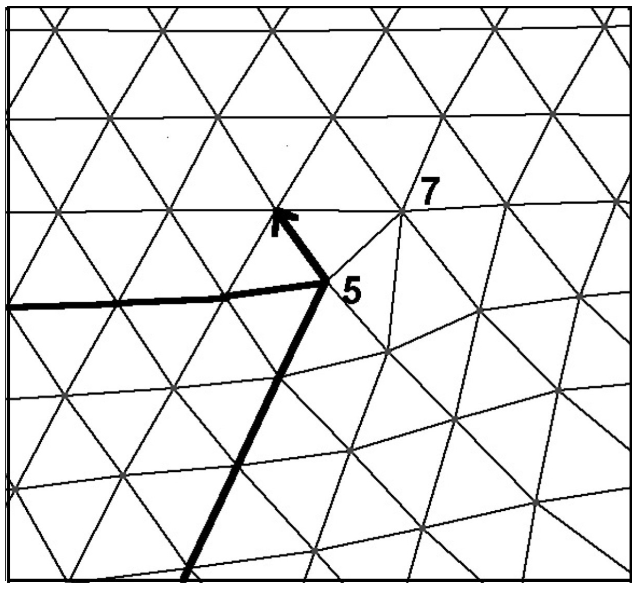
3.4. Grain Boundary Formation and Dynamics

Once the crystals impinge on each other at a time that depends on the concentration of the particles, it imposes the formation of the GBs. Before this time, the process of grain coarsening originated from the simple growth of the crystals above the critical size due to Ostwald ripening, acquiring particles from the surrounding fluid (see video 2). In Figure 10 it is shown the aspect of a grain boundary for t = 11,001. Note how the axes of symmetry of the two touching crystals do not coincide: the crystals are misaligned. This GB is not static; there is a continuous interchange of particles, crossing the boundary between the two crystals which, in turn, forces the boundary to move, even in the absence of an externally imposed strain. Thus, the GBs can be considered as fluctuating interfaces. At the particle level, it was proposed more than a century ago [96] that the metal crystalline grains in cast iron were separated by a thin layer of noncrystalline material “analogous to the condition of a greatly supercooled liquid”, what we now know as a glass-forming liquid. This observation has recently been proven via MD simulations [97] and experimentally in 2D [60] and 3D [59] by observing that the mean square displacement of a GB particle show diffusive behavior ($<r^2>\sim t$) for very short times, followed by a subdiffusive plateau indicative of particle trapping inside cages formed by the neighboring particles, and then crossing over to diffusive behavior again (also known as the α-relaxation regime) due to cage breaking. However, the long time diffusion constant is smaller compared to the short time diffusion. Furthermore, it was found that the diffusion of the GB particles along the GB was faster than across it [60]. Among the dynamical processes performed by a whole GB (i.e., the colective behavior of the particles that constitute the GB) that have been advanced, in the absence of an applied strain as in our case, that is, in the zero driving force limit [57,58,61,62,98], a one-dimensional random walk perpendicular to the GB has been highlighted by several researchers [57,61,62]. In their 3D computer simulations, Trautt et al. [61] were able to relate the interface mobility to the diffusion coefficient of this one-dimensional random walk, by exploiting a fluctuation-dissipation relation similar to the Stokes-Einstein relation. Starting with a planar interface perpendicular to the z direction and denoting the interface height profile as h($\mathit{r}$,t), where $\mathit{r}$ = $(x,y)$ is restricted to the interfacial plane, and by averaging over the x and y coordinates they obtain a mean square displacement on the z direction as $<h^2>=Dt$, with the diffusion coefficient

$$D=\frac{2M{k}_{B}T}{A}$$

(12)

where M is the mobility and A the area of their 3D GB. This mathematical development was validated with moleclular dynamics (MD) simulations of an initially flat grain boundary, with an attractive potential between the particles, and it was observed that the average interface position <h(t)> maintains a normal (Gaussian) distribution within each time interval considered [61]. It should be said, however, that their simulations were very short—what the MD simulations permitted—and lasted on the order of a few hundreds of picoseconds, corresponding to a movement of the mean interface position by several interatomic distances only. Skinner et al. [62] studied a two-dimensional experimental colloidal crystal, with repulsive interactions between the particles, with video microscopy. By the use of capillary wave theory they were able to obtain not only the mobility M of the grain boundary but also to extract its stiffness Γ, that relates the velocity v to the driving force, in this case the curvature κ: $v=M\mathrm{\Gamma }\kappa$. A thorough use of the capillary fluctuation method (CFM) [99]—widely used in studies of not only solid-liquid interfaces [100] but also of fluid-fluid surfaces [101,102], the Ising model [103] and amorphous polymer films [104]—aparently confirmed the one-dimensional random walk performed by the GB line on a direction perpendicular to it [62]. Another, very recent result [58] on the dynamics of the GBs for a two-dimensional colloidal crystal, is that the GBs with a maximum misorientation angle (~30${}^{\circ }$) show slow relaxation, while the boundary migration is much faster for asymmetrically sized domains separated by GBs with less misorientation.

In the present simulations the movement of some GB lines were followed for a long time and were found to perform not only a one-dimensional random walk but also a random rotation and even a deformation. In Figure 11a–d we are showing this situation. In the figures are shown the whole simulation box for the MC times of (a) 14,001, (b) 35,001, (c) 56,001 and (d) 98,001, The straight lines labeled A through D in the figures are drawn following the average position of some of the GBs; lines A through C were defined at the MC time of 14,001, when the corresponding GBs were already present, while line D was defined for the MC time of 35,001, once its corresponding GB was formed. That the lines A through D pass through the GBs at the mentioned times can be verified by zooming in the figure with the computer viewer. With the exception of GB A, whose movement is roughly perpendicular to the line A, for the other three GBs there is additionally a random rotation and a deformation of them. This should not be surprising since we are dealing with the movement of the GBs as coming from the interchange of particles between the two grains, crossing the GB that separates them. We should not expect the net crossing of particles at one end of the GB to be equal at the other end or, for that matter, at any point along the GB, since we are dealing with random events. Note that an evaluation during the course of time of $<h^2>$ for a GB with translation on the normal direction, with rotation and with deformation, could also lead to a diffusion law like $<h^2>=D^{\prime }t$. The line A was omitted in Figure 11d since, due to the healing of the extremes of the GB, the two grains convert into one bigger grain with some defects inside, a process that will be studied in the next section. We have observed that this healing occurs when the axes of symmetry of the two grains are not very misaligned.

3.5. Grain Coarsening by Dislocation Disappearance after Grain Boundary Healing

In Figure 12a, for the MC time 6101, two grains above the critical size that just started touching can be appreciated. In Figure 12b, for t = 6801, we can see on the left side of the grain boundary that the symmetry axes of the two grains are trying to align, although they do not succeed completely and their axes are still misaligned by a small angle.

The process of crystallization of some part of the grain boundary, in this case of the left side, is called the healing of the boundary. As time proceeds, the healing continues. In Figure 13a for the time t = 8001, now it is the right side of the boundary that apparently has also healed. This healing of the right boundary may occur from the slow and painful alignment, particle by particle, of the rows on the right side as it occurred on the left side, but perhaps helped by the rotation of the two grains as rigid bodies [105,106], driven by the torque exerted by the already healed left side. In Figure 13a we can see the formation of an amorphous vacancy inside the new crystalline grain formed by the union of the two original ones. However, this vacancy is not like the usual vacancies in which one only removes one particle of the crystal (or more adjacent particles, to have double or triple vacancies, etc.). In this last case the symmetry of the crystal grain remains unchanged. To corroborate that the the vacancy that appears in Figure 13a is more than just a vacancy, a Burgers circuit [107,108,109,110] is built, shown in Figure 13b, that in the crystalline space is just a polygon of equal sides. In this case we have tried to enclose the vacancy with a triangle, that could be equilateral if we had a perfect crystal symmetry, given that such Burgers circuit consists of three sides, each of a length of 12 lattice spacings. In the case of a perfect symmetry for the new crystalline grain, the initial and the final point of the Burgers circuit should coincide. This does not occur, as we can see in Figure 13b and, from the initial to the final point of the circuit (traversed counterclockwise, according to one of the conventions available in the literature [107,108]), we can draw a vector of roughly the size of a lattice spacing shown in the figure. This is called a Burgers vector. Conversely, the same Burgers vector could be obtained by traversing the circuit clockwise and defining it from the final to the initial point.

The fact that exists a Burgers vector different from zero indicates that the amorphous vacancy shown in Figure 13 contains a dislocation [107,108,109,110] which, for a 2D system like the one under study, has to be an edge dislocation, given that there are no screw dislocations in planar crystalline systems. Edge dislocations are generally described as extra half-rows (or extra half-planes in 3D) of particles coming from the crystal boundary all the way up to the dislocation core. For the triangular lattice case under study, the extra half-rows occur on the two symmetry axes which are not on the direction of the Burgers vector, as can be appreciated in Figure 13. The existence of these half-rows can be traced to the fact that the two symmetry axes that try to align belonging to each of the two “joining” crystals—closer to the perpendicular to the grain boundary line—make two angles, one above 180${}^{\circ }$ and the other below this value. Obviously, it is possible to accomodate more rows of particles on the greater than 180${}^{\circ }$ side than on the other. We have observed Burgers vectors with a size of two or more lattice spacings. In the present case of Figure 13, where the Burgers vector size is just one lattice spacing, indicates that there are just two more extra half-rows of particles (one for each of those two axes which are not on the direction of the Burgers vector), coming from the right side to the dislocation core than coming from the left side. The size in units of lattice spacings of the Burgers vector indicates the number of extra half-rows that come from one side than from the other, along one of the axes.

The dislocation shown in Figure 13 is somewhat more complex than the usual dislocations considered in the literature (see Figure 14)—consisting of two disclinations [28] of coordination 5 and 7—perhaps due to the randomness of the movement of our Brownian particles, which favors the formation of crystals with rough, fractal boundaries. Therefore, for other types of growth, it may be possible to obtain flat crystals (faceted in 3D) which produce smoother grain boundaries. In the following we will obtain dislocations even more complex than the one shown in Figure 13 and will be referred to as complex dislocations (CD). A CD is just a dislocation like that in Figure 14 mixed with vacancies. To better understand what a CD is, a Delaunay triangulation of a CD will be shown below in Figure 20.

A dislocation has associated with it stress and strain fields surrounding the dislocation core [107]. The existence of distortion around a dislocation implies that the crystal is not in its lowest energy state. Consequently, energy is stored in the strained region around the dislocation, and the total strain energy of the body in the absence of external stresses may be called the elastic energy of the dislocation. We will now describe a particular process we have found for the crystal to get rid of dislocations and, in this way, to liberate the extra energy coming from them and increase its symmetry. This will lead to grain coarsening, since the dislocation-containing crystal came from the merging of two smaller grains.

In panel (a) of Figure 15 is shown the same crystal grain as in Figure 13, but now for the time t = 8501. We can observe the way that the crystal has opted to get rid of the dislocation it contains. It opens up a small channel in the zone where there are less rows of particles, directed to the zone closer to the boundary with the surrounding fluid. Such channel starts to be filled up with particles, as can be appreciated in panel (b) of the same figure, coming from the walls of the same channel as well as from particles of the surrounding fluid. Finally, in Figure 16 for the time t = 10,501 it can be observed that the channel has disappeared and the the crystal has healed completely. It is interesting to note that the CDs (containing vacancies) are more mobile than pure vacancies. In Figure 15a (t = 8501) the formation of a pure vacancy can be observed around the coordinates (237, 409) such that, when the time reached t = 10,501 (Figure 16), it only moved to the coordinates (235, 411). This indicates that pure vacancies are more entrenched to the crystal than the complex dislocations, which are more mobile. We also note, in the upper-right corner of Figure 16, the formation of a new, bigger grain boundary that will be described next.

In Figure 17a, for the time t = 9001, it can be observed two crystal grains that are starting to touch, the lower being the one we have just described in its formation. At the time t = 28,001 (Figure 17b) we can see that a wide GB has been established, which has not undergone the healing processs. However, by waiting up to the time t = 68,001 (Figure 17c), the healing process has occurred in both extremes, enclosing in this way four complex unit dislocations with the same burguers vector pointing on the upper-right direction. This can be observed in Figure 17d, where are shown the four Burgers circuits. In fact, if we could enclose the four CDs with a single Burgers circuit, we would obtain a Burgers vector pointing in the same direction with a magnitude of four lattice spacings. This comes from the fact that the Burgers vectors can be added to obtain the magnitude of the total dislocation [107,108,109,110]. It can also be noted that the four Burgers vectors lie along the same symmetry axis of the Burgers vector studied before (Figure 13b), but pointing on the opposite direction. That they are found on the same symmetry axis as before indicates that such axis is the closest to the perpendicular to the GB line in Figure 17b. The opposite direction comes from the fact the angle greater than 180^o is now situated on the opposite side as the case before.

We will now see the way in which the crystal gets rid of the four CDs found inside the crystal. In Figure 18a, for the time t = 72,501, it can be seen that rightmost CD has just “gone out” from the crystal when the boundary with the fluid has just opened up. In Figure 18b, now for the time t = 80,001, is observed that such rightmost boundary has healed and also that the leftmost dislocation has migrated upwards, going out from the left boundary. At the time t = 80,501 (Figure 18c) we can see that this left boundary has healed completely. In Figure 18d, for the time t = 89,001, we see that the CD in the lower right zone has gone out, this time from the right boundary, leaving therefore a single dislocation in the very interior of the crystal grain. In Figure 19 we are following up the movement of this dislocation noticing that, given that it does not “feel” the presence of the boundary with the fluid, it stays migrating inside the grain, probably in a random way. Finally, in Figure 19c for the time t = 101,001, it is observed that it is very close to the boundary with the fluid to go out from there and disappear. In Figure 19d for the time t = 101,501 the CD has already disappeared. Now the symmetry axes of the crystal grain are very well defined and the only imperfections of such crystal consist of a few pure vacancies, that do not destroy its symmetry. However, in the upper part of the figure it can be observed the formation of new GBs with other crystal grains as well as the formation of a triple junction. By observing the angles of misalignment in Figure 17c and Figure 18d, we note how the subsequent disappearance of single CDs keeps restoring orientational order. This is different from the KTHNY mechanism of melting (and solidification) since dislocations are produced (and annihilated) in anti-parallel pairs, which do not destroy orientational order. On the other hand, in our case, the Burgers vectors of the subsequently disappearing dislocations point on the same direction. Therefore, in order to restore the orientational order, we need them to disappear across the boundary of the crystal grain. As previously announced, in Figure 20 it is shown the Delaunay triangulation of a CD, the third from the left in Figure 17c,d.

We have found that this process of grain coarsening by GB disappearance, for a reasonable elapsed time, occurs under two conditions: (1) That the symmetry axes of the two crystals whose GB is going to disappear are more or less aligned, i.e., that the angle formed by such axes do not exceed 12${}^{\circ }$–15${}^{\circ }$ say, that is a LAGB; (2) That the GB is not too large. Otherwise, in principle it would be possible the fusion of two of these crystals, for which one would need to wait for an extremely long time, both experimentally and simulationally. In Figure 21 is shown the whole simulation box for the MC time t = 111,001. We can see that the system consists of 6 crystalline grains (taking into account the periodicity of the box boundaries), all of which make a boundary with two or more grains, except one of them. However, this particular grain makes a boundary with another one whose symmetry axis makes an angle close to the maximum angle of 30${}^{\circ }$ with the first one, something that can be verified by zooming in the figure. Therefore, it would be very difficult the fusion of those two grains. This is the reason why most metals and another crystals are in reality polycrystals, consisting on grains separated by GBs. In an experimental system, particularly in the atomic crystals case, we can have a large cellular structure of crystalline grains separated by a large network of GBs. How relevant the results presented here are to that case is difficult to asses. However, in order to perform a simulation for that case, we need to start with many millions of particles, which for the time being is not computationally accessible. In this case one needs to resort to some theoretical models that will be reviewed in the next section which, of course, would need to include the correct ingredients to obtain physically reasonable results.

3.6. Some Theoretical Developments of Grain Coarsening

On the theoretical side, there have been a number of advances on the description of grain growth and coarsening. Several techniques for the computer simulation of grain growth have been developed, including a kinetic q-state Potts model on a regular lattice [111,112,113], with a Hamiltonian defined by

$$H=-\frac{J}{2}\sum _i^N\sum _j^{nn}({\delta }_{s_i{s}_j}-1)s_i,s_j=1,2,\dots ,q$$

(13)

which is well known to form domains of different spin numbers [114]. $s_k$, the corresponding spin number of each lattice site represents a particular crystal orientation in which the site is embedded. ${\sum }_i^{{}_N}$ is the sum over all lattice sites and ${\sum }_j^{nn}$ is the sum over all nearest neighbors of the site i. Lattice sites $s_i$ that are adjacent to sites having different grain orientations $s_j\ne s_i$ were defined to be separated by a HAGB. On the other hand, if a site is surrounded by sites with the same orientation, it is located in the grain interior. The use of a kinetic Monte carlo simulation for this model allowed them to obtain different growing grains covering the whole lattice. Vertex models have also been employed to describe the grain coarsening of grain structures [115,116]. In this case the vertices of the disordered lattice correspond to triple junctions between grains. Weygand et al. [116] also considered a set of “virtual vertices” discretizing the GBs between pairs of triple points. The motion of the virtual vertices allowed them to obtain GBs which are not exclusively straight lines but that could have some curvature. D. Raabe [117] applied the cellular automata model to the study of grain growth and recrystallization phenomena [118]. It starts from a regular array of lattice points that can be regarded, for example, as atomic particles (or, as in our case, colloidal particles). Each lattice point is characterized in terms of a set of generalized state variables which, for our case, could be crystal orientations. The dynamical evolution of the automaton takes place through the application of deterministic or probabilistic transformation rules that act on the state of each lattice point. These rules determine the state of a lattice point as a function of its (discrete time) previous state and the state of the neighboring sites. The use of this method has provided interesting results for the simulation of primary static recrystallization in aluminum [119] and for the yield surface of aluminum polycrystals during recrystallization [120]. Another approach that should be highlighted is the use of phase field models to describe the process of grain coarsening [121]. Kobayashi et al. [122] employed a phase field to describe crystallization, impingement and GB formation in 1D and extended it to 2D [123], taking into account the rotation of the crystal grains as rigid bodies [105,106]. Later, the authors extended the method to the evolution of a polycrystalline microstructure by impingement, followed by grain boundary migration and grain rotation [124]. Extensions of the method to 3D have also been developed [125,126,127]. More on rotation-induced growth can be found in [128]. Recent reviews on the subject are given in Gránásy et al. [129] and Singer-Loginova and Singer [130].

4. Discussion and Conclusions

As we have seen, with a simple kinetic MC simulation with Metropolis dynamics it is possible to retrieve and visualize in 2D all known different subprocesses undergone by a crystallizing system of colloidal particles (or colloidal-like particles, like proteins), interacting with a short-ranged attraction. First, before the nucleation process begins, a fluid-fluid phase separation is obtained, with the coexistence of dense and rarefied zones of the fluid. Afterwards, the nucleation process starts at the denser portions of the phase separated system. We have shown how to derive the critical crystallite size with a knowledge of the position of the particles as a function of time, inspired by previous work [46,70]. A use was made of the fractality of the crystallite boundaries in order to obtain the line tension and the chemical potential difference between the disordered and crystalline phases. It was also possible to contemplate the process of Ostwald ripening, noticing how some of the supercritical crystals become subcritical as the time proceeds, due to the fact that the disordered phase becomes less and less dense and hence undersaturated for those crystals, which makes them prone to shrink and disappear. The formation of the GBs was visualized when two nearby crystals impinge on each other during their growth. As there is an interchange of particles between the two crystals forming a GB, it becomes a fluctuating interface, undergoing a random translation on a direction perpendicular to it, as well as a random rotation and deformation. Subsequently, for LAGBs sometimes there was a healing of the extremes of the GBs and, hence, there was a trapping of CDs inside the new imperfect crystal grain, formed by the merging of the two original ones. Those CDs migrate very readily inside the new grain, until they find the boundary between the grain and the disordered phase, and escape from there. Once the new grain has gotten rid of all CDs, it becomes a new, larger crystal grain, whose only imperfections consist of simple vacancies, which do not destroy the symmetry of the lattice. Arguably, this process of trapping CDs, CDs migration and going out from the boundary with the fluid could be called a coalescence. Once the LAGBs have disappeared, we end up with the final product of the crystallizing system: the polycrystal. We have treated the crystallization of colloidal particles interacting with an attractive potential, in which case the final polycrystal does not fill the whole simulation box, leaving a space with a dilute disordered phase. This coexistence of two phases, one ordered and the other disordered is indicative of a first order phase transition, which includes crystal nucleation and a critical nucleation barrier, as we have seen. Let us make a brief review of the type of phase transitions we can have with attractive and repulsive isotropic potentials between the particles, both for 3D and 2D.

In 3D, there is homogeneous or heterogeneous nucleation of supercooled fluids to the periodic structure. This phase transition has been extensively studied, both for attractive and repulsive potentials (including hard spheres), and has been found to be first order, with ordered and disordered phases coexisting in equilibrium and with a nucleation process as the one we have studied here. For example, in the hard sphere case, the volume fractions of freezing (${\varphi }_f$) and melting (${\varphi }_m$) do not depend on temperature and are around ${\varphi }_f\simeq 0.494$ and ${\varphi }_m\simeq 0.545$ [131]. In between those two concentrations there is coexistence of ordered and disordered phases. Likewise, for attractive and repulsive potentials in 3D a first order phase transition with nucleation has been studied in numerous works (e.g., in references [46,132,133,134,135,136,137,138,139,140] just to cite a few). As mentioned in the introduction, in 3D we can have a two-step nucleation if the interaction potential has a short-range attraction [31,32,33,34,38,39,40,41,42], which induces a metastable fluid-fluid phase separation before crystal nucleation starts. In the case of hard spheres that do not present this phase separation, it has however remarkably been found with computer simulations that the formation of dense, amorphous clusters (whose origin needs to be explained, if it comes by simple density fluctuations or by some other mechanism) is the only prerequisite to initiate the crystal nucleation process inside those clusters [141].

In 2D, it has been noted in the introduction that a short-range attraction can also induce two-step crystal nucleation in the denser portions of the fluid-fluid phase separated system [35,36,37,70], leading to a first order crystallization transition, with nucleation and a nucleation barrier at the critical size. There is also phase coexistence between the polycrystal and the dilute disordered phase (e.g., Figure 21), indicative of a first order transition. For the 2D repulsive case, the crystallization process apparently does not follow the same path. In [30,76], the authors use super-paramagnetic colloids confined to a flat water-air interface, such that an applied magnetic field perpendicular to the interface acts as the inverse of temperature, due to the alignment of the magnetic repulsive dipoles along the magnetic field. As the authors state, immediately after the sudden quench to a large magnetic field (low temperature) begins the formation of a large number of small crystallites. In this case, no nucleation barrier which defines a critical nucleus size has to be overcome by a fluctuation [76]. In a first period of time, the number and the size of the crystallites increase in the course time, up to the point where the crystallites or crystals start to touch [30]. Then a ripening process starts where the particles are reorganized and the large crystals grow at the expense of the small ones, in a process resembling Ostwald ripening but with touching crystals. Afterwards, the number of crystals decreases in this second stage and their size increases at a lower rate. It should be noted that there is no phase coexistence between the polycrystal and a disordered phase, and the whole polycrystal fills the whole experimental box.

Now, what happens to the melting (crystallization) of 2D particles when the heating (cooling) rate is made to be extremely slow, such that the system always remains in thermal equilibrium? As mentioned in the introduction, with the exception of some works [12,13,14,15] which find a first order transition, most researchers find two phase transitions with a hexatic phase in between the fluid and the crystal phases, in accord with the KTHNY theory [27,28,29]. Some researchers find the two transitions to be continuous [16,17,18,19,20,21], while some others [22,23,24,25,26] find one or the two transitions to be first order (indicating a coexistence of the phases at the transition point), depending on the repulsive interaction potential. To inquire about the crossover from a crystallization transition for a sudden quench—as described in the last paragraph—to a KTHNY type of transition for a very slow cooling rate, Deutschländer et al. [142] have studied the crystallization process when varying the cooling rate by three orders of magnitude. Assuming that the two continuous phase transitions in the KTHNY theory are second order-like, there should be a critical slowing down with a correlation time becoming longer and diverging, the closer we are to the transition point. In this case, a Kibble-Zurek mechanism should apply (which has been used not only in condensed matter transitions like the normal to superfluid transition in liquid helium, but in fact it had its origin in the cosmological transition during the cooling down of the early universe). If the cooling down of the colloidal system is very fast, the system does not have time to rearrange into the KTHNY type of transition and the hexatic phase (with their separated opposite-Burgers-vector dislocations) is lost, while if the cooling rate is very slow, the system can follow this transition very closely. In their work [142], the authors have tested different predictions of the Kibble-Zurek mechanism. Finally, to the best knowledge of the present author, all the works pertaining to the test of the KTHNY theory—either experimentally or simulationally—that unambiguously find a hexatic phase have been made with repulsive colloidal interactions. The question of what would happen with an attractive potential between the colloidal particles, when melting a monocrystal (or crystallizing a fluid) by heating it up (or cooling it down) very slowly, remains therefore as an open question and is beyond the scope of the present article. In the case that a KTHNY type of transition could be found for a very slow cooling rate, we expect that the Kibble-Zurek mechanism would tell us again that the KTHNY transition will be lost—for a sudden quench to a lower temperature—in favor of the first order transition we have just seen in the present work.

From a technological perspective, polycrystals are profitable since precise control over their mechanical, optical and electrical properties can be achieved by tailoring the morphology of the grain network. Therefore, understanding GB dynamics and its implications for grain growth stays as one of the primary goals of materials research. Among the tools to connect single particle dynamics at GBs and grain growth, the transmission electron microscopy (TEM) has been widely used for studying grain growth in atomic polycrystals, but is very frequently unable to probe particle dynamics at buried GBs, due to the small particle size and the very fast atomic motion [143]. MD simulations of atomic particles can model systems realistically, but are resricted to small systems and short time scales [61,130,144]. Perhaps, one drawback of the above mentioned theoretical models is the absence of a complete connection between single particle dynamics at GBs and grain growth, in the sense that they have been so far unable to capture several microscopic details of the particle motion and relate them to grain growth and GB dynamics. Nonetheless, the phase field model seems to be a promising procedure for calculating mesoscopic phenomena, since it has been capable of rendering realistic-looking dendritic growth, grain growth and several other phenomena occurring in metals [130]. However, the process we have seen for “grain coarsening by dislocation disappearance after GB healing”, which arguably can be regarded as a “coalescence with a vanishing GB”, has not been introduced as an input into the above theoretical models [125,130]. Also, the glassy dynamics of the particles inside the GBs [59,60,97] has not been considered, as far as the author is aware. It seems that the models consider the grain coarsening phenomena merely as a result of boundary movement, which makes the smaller grains to shrink and disappear (the T2 processes considered in Stavans review of cellular structures [56]), without explicitly considering coalescence. Perhaps, the introduction of a balanced dynamics, considering not only the T2 processes but also coalescence with vanishing GBs would be beneficial to those models.

Experimentally, colloidal particles have shown to be a useful model system where to probe atomistic phenomena [3,4,5,6,7]. Their large size (∼$\mathsf{\mu }$m) and slow motion (~s) allow us to use simple optical techniques, like video microscopy, to study the crystallization phenomena. The corresponding simulational counterpart of the colloidal study is the Brownian dynamics method that, as we have seen, is equivalent to a MC simulation with Metropolis dynamics. Therefore, in the near future we should expect to see a growing interest in the use of colloidal particles to test atomistic phenomena, like crystallization, with the aid of simple imaging techniques. There are however many challenges to overcome in the study of colloidal polycrystals, which will merit the intellectual effort due to their practical application as model systems.

References

1. Pieranski, P. Colloidal crystals. Contemp. Phys. 1983, 24, 25–73. [Google Scholar] [CrossRef]
2. Gasser, U. Crystallization in three- and two-dimensional colloidal suspensions. J. Phys. Condens. Matter 2009, 21, 203101. [Google Scholar] [CrossRef] [PubMed]
3. Schall, P.; Cohen, I.; Weitz, D.A.; Spaepen, F. Visualization of dislocation dynamics in colloidal crystals. Science 2004, 305, 1944–1948. [Google Scholar] [CrossRef] [PubMed]
4. Schall, P.; Cohen, I.; Weitz, D.A.; Spaepen, F. Visualizing dislocation nucleation by indenting colloidal crystals. Nature 2006, 440, 319–323. [Google Scholar] [CrossRef] [PubMed]
5. Suresh, S. Colloid model for atoms. Nat. Mater. 2006, 5, 253–254. [Google Scholar] [CrossRef] [PubMed]
6. Schall, P. Laser difraction microscopy. Rep. Prog. Phys. 2009, 72, 076601. [Google Scholar] [CrossRef]
7. Wang, Z.; Wang, F.; Peng, Y.; Zheng, Z.; Han, Y. Imaging the homogeneous nucleation during the melting of superheated colloidal crystals. Science 2012, 338, 87–90. [Google Scholar] [CrossRef] [PubMed]
8. See for example Crystallization of Nucleic Acids and Proteins: A Practical Approach, 2nd ed.; Ducruix, A.; Giegé, R. (Eds.) Oxford University Press: Oxford, UK, 2000.
9. Pieranski, P. Two-dimensional interfacial colloidal crystals. Phys. Rev. Lett. 1980, 45, 569–572. [Google Scholar] [CrossRef]
10. Grimes, C.C.; Adams, G. Evidence for a liquid-to-crystal phase transition in a classical, two-dimensional sheet of electrons. Phys. Rev. Lett. 1979, 42. [Google Scholar] [CrossRef]
11. Onoda, G.Y. Direct observation of two-dimensional, dynamical clustering and ordering with colloids. Phys. Rev. Lett. 1985, 55, 226–229. [Google Scholar] [CrossRef] [PubMed]
12. Saito, Y. Monte Carlo studies of two-dimensional melting: Dislocation vector systems. Phys. Rev. B 1982, 26, 6239–6253. [Google Scholar] [CrossRef]
13. Chui, S.T. Grain-boundary theory of melting in two dimensions. Phys. Rev. Lett. 1982, 48, 933–935. [Google Scholar] [CrossRef]
14. Tang, Y.; Armstrong, A.J.; Mockler, R.C.; O’Sullivan, W.J. Free-expansion melting of a colloidal monolayer. Phys. Rev. Lett. 1989, 62, 2401–2404. [Google Scholar] [CrossRef] [PubMed]
15. Lansac, Y; Glaser, M.A.; Clark, N.A. Discrete elastic model for two-dimensional melting. Phys. Rev. E 2006, 73, 041501. [Google Scholar] [CrossRef] [PubMed]
16. Murray, C.A.; van Winkle, D.H. Experimental observation of two-stage melting in a classical two-dimensional screened coulomb system. Phys. Rev. Lett. 1987, 58, 1200–1203. [Google Scholar] [CrossRef] [PubMed]
17. Kusner, R.E.; Mann, J.A.; Kerins, J.; Dahm, A.J. Two-stage melting of a two-dimensional colloidal lattice with dipole interactions. Phys. Rev. Lett. 1994, 73, 3113–3116. [Google Scholar] [CrossRef] [PubMed]
18. Bladon, P.; Frenkel, D. Dislocation unbinding in dense two-dimensional crystals. Phys. Rev. Lett. 1995, 74, 2519–2522. [Google Scholar] [CrossRef] [PubMed]
19. Zahn, K.; Lenke, R.; Maret, G. Two-stage melting of paramagnetic colloidal crystals in two dimensions. Phys. Rev. Lett. 1999, 82, 2721–2724. [Google Scholar] [CrossRef]
20. Von Grünberg, H.H.; Keim, P.; Zahn, K.; Maret, G. Elastic behavior of a two-dimensional crystal near melting. Phys. Rev. Lett. 2004, 93, 255703. [Google Scholar] [CrossRef] [PubMed]
21. Keim, P.; Maret, G.; von Grünberg, H.H. Frank’s constant in the hexatic phase. Phys. Rev. E 2007, 75, 031402. [Google Scholar] [CrossRef] [PubMed]
22. Marcus, A.H.; Rice, S.A. Observations of first-order liquid-to-hexatic and hexatic-to-solid phase transitions in a confined colloidal suspension. Phys. Rev. Lett. 1996, 77, 2577–2580. [Google Scholar] [CrossRef] [PubMed]
23. Lin, B.J.; Chen, L.J. Phase transitions in two-dimensional colloidal particles at oil/water interfaces. J. Chem. Phys. 2007, 126, 034706. [Google Scholar] [CrossRef] [PubMed]
24. Bernard, E.P.; Krauth, W. Two-step melting in two dimensions: First-order liquid-hexatic transition. Phys. Rev. Lett. 2011, 107, 155704. [Google Scholar] [CrossRef] [PubMed]
25. Engel, M.; Anderson, J.A.; Glotzer, S.C.; Isobe, M.; Bernard, E.P.; Krauth, W. Hard-disk equation of state: First-order liquid-hexatic transition in two dimensions with three simulation methods. Phys. Rev. E 2013, 87, 042134. [Google Scholar] [CrossRef] [PubMed]
26. Kapfer, S.C.; Krauth, W. Two-dimensional melting: From liquid-hexatic coexistence to continuous transitions. Phys. Rev. Lett. 2015, 114, 035702. [Google Scholar] [CrossRef] [PubMed]
27. Kosterlitz, J.M.; Thouless, D.J. Ordering, metastability and phase transitions in two-dimensional systems. J. Phys. C Solid State Phys. 1973, 6, 1181–1203. [Google Scholar] [CrossRef]
28. Nelson, D.R.; Halperin, B.I. Dislocation-mediated melting in two dimensions. Phys. Rev. B 1979, 19, 2457–2484. [Google Scholar] [CrossRef]
29. Young, A.P. Melting and the vector coulomb gas in two dimensions. Phys. Rev. B 1979, 19, 1855–1866. [Google Scholar] [CrossRef]
30. Dillman, P.; Maret, G.; Keim, P. Polycrystalline solidification in a quenched 2D colloidal system. J. Phys. Condens. Matter 2008, 20, 404216. [Google Scholar] [CrossRef]
31. Lekkerkerker, H.N.W.; Poon, W.C.K.; Pusey, P.N.; Stroobants, A.; Warren, P.B. Phase behaviour of colloid + polymer mixtures. Europhys. Lett. 1992, 20, 559–564. [Google Scholar] [CrossRef]
32. Hagen, M.H.J.; Frenkel, D. Determination of phase diagrams for the hard-core attractive Yukawa system. J. Chem. Phys. 1994, 101, 4093–4097. [Google Scholar] [CrossRef]
33. Ilett, S.M.; Orrock, A.; Poon, W.C.K.; Pusey, P.N. Phase behavior of a model colloid-polymer mixture. Phys. Rev. E 1995, 51, 1344–1352. [Google Scholar] [CrossRef]
34. Asherie, N.; Lomakin, A.; Benedek, G.B. Phase diagram of colloidal solutions. Phys. Rev. Lett. 1996, 77, 4832–4835. [Google Scholar] [CrossRef] [PubMed]
35. Hobbie, E.K. Metastability and depletion-driven aggregation. Phys. Rev. Lett. 1998, 81, 3996–3999. [Google Scholar] [CrossRef]
36. Zhang, T.H.; Liu, X.Y. How does a transient amorphous precursor template crystallization. J. Am. Chem. Soc. 2007, 129, 13520–13526. [Google Scholar] [CrossRef] [PubMed]
37. Savage, J.R.; Dinsmore, A.D. Experimental evidence for two-step nucleation in colloidal crystallization. Phys. Rev. Lett. 2009, 102, 198302. [Google Scholar] [CrossRef] [PubMed]
38. Berland, C.R.; Thurston, G.M.; Kondo, M.; Broide, M.L.; Pande, J.; Ogun, O.; Benedek, G.B. Solid-liquid phase boundaries of lens protein solutions. Proc. Natl. Acad. Sci. USA 1992, 89, 1214–1218. [Google Scholar] [CrossRef] [PubMed]
39. Ten Wolde, P.R.; Frenkel, D. Enhancement of protein crystal nucleation by critical density fluctuations. Science 1997, 277, 1975–1978. [Google Scholar] [CrossRef] [PubMed]
40. Talanquer, V.; Oxtoby, D.W. Crystal nucleation in the presence of a metastable critical point. J. Chem. Phys. 1998, 109, 223–227. [Google Scholar] [CrossRef]
41. Galkin, O.; Vekilov, P.G. Control of protein crystal nucleation around the metastable liquid-liquid phase boundary. Proc. Natl. Acad. Sci. USA 2000, 97, 6277–6281. [Google Scholar] [CrossRef] [PubMed]
42. Lomakin, A.; Asherie, N.; Benedek, G.B. Liquid-solid transition in nuclei of protein crystals. Proc. Natl. Acad. Sci. USA 2003, 100, 10254–10257. [Google Scholar] [CrossRef] [PubMed]
43. Mao, Y.; Cates, M.E.; Lekkerkerker, H.N.W. Depletion force in colloidal systems. Phys. A 1995, 222, 10–24. [Google Scholar] [CrossRef]
44. Rosenbaum, D.; Zamora, P.C.; Zukoski, C.F. Phase behavior of small attractive colloidal particles. Phys. Rev. Lett. 1996, 76, 150–153. [Google Scholar] [CrossRef] [PubMed]
45. Kelton, K.F. Crystal nucleation in liquids and glasses. In Solid State Physics; Ehrenreich, H., Turnbull, D., Eds.; Academic Press: San Diego, CA, USA, 1991; Volume 45, pp. 75–177. [Google Scholar]
46. Gasser, U.; Weeks, E.R.; Schofield, A.; Pusey, P.N.; Weitz, D.A. Real-space imaging of nucleation and growth in colloidal crystallization. Science 2001, 292, 258–262. [Google Scholar] [CrossRef] [PubMed]
47. Rubin-Zuzic, M.; Morfill, G.E.; Ivlev, A.; Pompl, R.; Klumov, B.A.; Bunk, W.; Thomas, H.M.; Rothermel, H.; Havnes, O.; Fouquet, A. Kinetic Develpment of crystallization fronts in complex plasmas. Nat. Phys. 2006, 2, 181–185. [Google Scholar] [CrossRef]
48. Yau, S.T.; Vekilov, P.G. Quasi-planar nucleus structure in apoferritin crystallization. Nature 2000, 406, 494–497. [Google Scholar] [PubMed]
49. Pan, A.C.; Chandler, D. Dynamics of nucleation in the Ising model. J. Phys. Chem. B 2004, 108, 19681–19686. [Google Scholar] [CrossRef]
50. Ostwald, W. Studien uber die Bildung und Umwandlung fester Korper. Z. Phys. Chem. 1897, 22, 289–330. [Google Scholar]
51. Penn, R.L.; Banfield, J.F. Morphology development and crystal growth in nanocrystalline aggregates under hydrotermal conditions: Insights from titania. Geochim. Cosmochim. Acta 1999, 63, 1549–1557. [Google Scholar] [CrossRef]
52. Madras, G.; McCoy, B.J. Growth and ripening kinetics of crystalline polymorphs. Cryst. Growth Des. 2003, 3, 981–990. [Google Scholar] [CrossRef]
53. Huang, F.; Zhang, H.; Banfield, J.F. Two-stage crystal-growth kinetics observed during hydrotermal coarsening of nanocrystalline ZnS. Nano Lett. 2003, 3, 373–378. [Google Scholar] [CrossRef]
54. Streets, A.M.; Quake, S.R. Ostwald ripening of clusters during protein crystallization. Phys. Rev. Lett. 2010, 104, 178102. [Google Scholar] [CrossRef] [PubMed]
55. Iacopini, S.; Palberg, T.; Schöpe, H.J. Ripening-dominated crystallization in polydisperse hard-sphere-like colloids. Phys. Rev. E 2009, 79, 010601. [Google Scholar] [CrossRef] [PubMed]
56. Stavans, J. The evolution of cellular structures. Rep. Prog. Phys. 1993, 56, 733–789. [Google Scholar] [CrossRef]
57. Gokhale, S.; Nagamanasa, K.H.; Ganapathy, R.; Sood, A.K. Grain growth and grain boundary dynamics in colloidal polycrystals. Soft Matter 2013, 9, 6634–6644. [Google Scholar] [CrossRef]
58. Edwards, T.D.; Yang, Y.; Beltran-Villegas, D.J.; Bevan, M.A. Colloidal crystal grain boundary formation and motion. Sci. Rep. 2014, 4. [Google Scholar] [CrossRef] [PubMed]
59. Nagamanasa, K.H.; Gokhale, S.; Ganapathy, R.; Sood, A.K. Confined glassy dynamics at grain boundaries in colloidal crystals. Proc. Natl. Acad. Sci. USA 2011, 108, 11323–11326. [Google Scholar] [CrossRef] [PubMed]
60. Skinner, T.O.E.; Aarts, D.G.A.L.; Dullens, R.P.A. Supercooled dynamics of grain boundary particles in two-dimensional colloidal crystals. J. Chem. Phys. 2011, 135, 124711. [Google Scholar] [CrossRef] [PubMed]
61. Trautt, Z.T.; Upmanyu, M.; Karma, A. Interface mobility from interface random walk. Science 2006, 314, 632–635. [Google Scholar] [CrossRef] [PubMed]
62. Skinner, T.O.E.; Aarts, D.G.A.L.; Dullens, R.P.A. Grain-boundary fluctuations in two-dimensional colloidal crystals. Phys. Rev. Lett. 2010, 105, 168301. [Google Scholar] [CrossRef] [PubMed]
63. Porter, D.A.; Easterling, K.E. Phase Transformations in Metals and Alloys, 2nd ed.; CRC Press: Boca Raton, FL, USA, 1992. [Google Scholar]
64. Kikuchi, K.; Yoshida, M.; Maekawa, T.; Watanabe, H. Metropolis Monte Carlo method as a numerical technique to solve the Fokker-Planck equation. Chem. Phys. Lett. 1991, 185, 335–338. [Google Scholar] [CrossRef]
65. Kikuchi, K.; Yoshida, M.; Maekawa, T.; Watanabe, H. Metropolis Monte Carlo method for Brownian dynamics simulation generalized to include hydrodynamics interactions. Chem. Phys. Lett. 1992, 196, 57–61. [Google Scholar] [CrossRef]
66. Yoshida, M.; Kikuchi, K. Metropolis Monte Carlo Brownian dynamics simulation of the ion atmosphere polarization around a rodlike polyion. J. Phys. Chem. 1994, 98, 10303–10306. [Google Scholar] [CrossRef]
67. Metropolis, N.; Rosenbluth, A.W.; Rosenbluth, M.N.; Teller, A.H.; Teller, E. Equation of state calculations by fast computing machines. J. Chem. Phys. 1953, 21, 1087–1092. [Google Scholar]
68. Honeycutt, J.D.; Andersen, H.C. The effect of periodic boundary conditions on homogeneous nucleation observed in computer simulations. Chem. Phys. Lett. 1984, 108, 535–538. [Google Scholar] [CrossRef]
69. Honeycutt, J.D.; Andersen, H.C. Small system size artifacts in the molecular dynamics simulation of homogeneous crystal nucleation in supercooled atomic liquids. J. Phys. Chem. 1986, 90, 1585–1589. [Google Scholar] [CrossRef]
70. González, A.E.; Ixtlilco-Cortés, L. Fractal structure of the crystalline-nuclei boundaries in 2D colloidal crystallization: Computer simulations. Phys. Lett. A 2012, 376, 1375–1379. [Google Scholar] [CrossRef]
71. Halperin, B.I.; Nelson, D.R. Theory of two-dimensional melting. Phys. Rev. Lett. 1978, 41, 121–124. [Google Scholar] [CrossRef]
72. Fraser, D.P.; Zuckermann, M.J.; Mouritsen, O.G. Simulation technique for hard-disk models in two dimensions. Phys. Rev. A 1990, 42, 3186–3195. [Google Scholar] [CrossRef] [PubMed] [Green Version]
73. Jaster, A. Computer simulation of the two-dimensional melting transition using hard disks. Phys. Rev. E 1999, 59, 2594–2602. [Google Scholar] [CrossRef]
74. Terao, T.; Nakayama, T. Crystallization in a quasi-two-dimensional colloidal system at an air-water interface. Phys. Rev. E 1999, 60, 7157–7162. [Google Scholar] [CrossRef]
75. Huerta, A.; Naumis, G.G.; Wasan, D.T.; Henderson, D.; Trokhymchuk, A. Attraction driven disorder in a hard-core colloidal monolayer. J. Chem. Phys. 2004, 120, 1506–1510. [Google Scholar] [CrossRef] [PubMed]
76. Dillman, P.; Maret, G.; Keim, P. Two-dimensional colloidal systems in time-dependent magnetic fields. Eur. Phys. J. Spec. Top. 2013, 222, 2941–2959. [Google Scholar] [CrossRef]
77. Lutsko, J.F.; Nicolis, G. Theoretical evidence for a dense fluid precursor to crystallization. Phys. Rev. Lett. 2006, 96, 046102. [Google Scholar] [CrossRef] [PubMed]
78. Mandelbrot, B.B. The Fractal Geometry of Nature; W. H. Freeman & Co.: San Francisco, FL, USA, 1988. [Google Scholar]
79. González, A.E.; Martínez-López, F.; Moncho-Jordá, A.; Hidalgo-Álvarez, R. Two-dimensional colloidal aggregation: Concentration effects. J. Colloid Interface Sci. 2002, 246, 227–234. [Google Scholar] [CrossRef] [PubMed]
80. González, A.E.; Martínez-López, F.; Moncho-Jordá, A.; Hidalgo-Álvarez, R. Concentration effects on two- and three-dimensional colloidal aggregation. Phys. A 2002, 314, 235–245. [Google Scholar] [CrossRef]
81. Lifshitz, I.M.; Slyozov, V.V. The kinetics of precipitation from supersaturated solid solutions. J. Phys. Chem. Solids 1961, 19, 35–50. [Google Scholar] [CrossRef]
82. Wagner, C. Theorie de alterung von niederschlägen durch umlösen. Ber. Bunsen-Ges. Phys. Chem. 1961, 65, 581–591. [Google Scholar]
83. Söhnel, O.; Garside, J. Precipitation; Butterworth-Heinemann: Oxford, UK, 1992. [Google Scholar]
84. Ng, J.D.; Lorber, B.; Witz, J.; Theóbald-Dietrich, A.; Kern, D.; Giegé, R. The crystallization of biological macromolecules from precipitates: Evidence for Ostwald ripening. J. Cryst. Growth 1996, 168, 50–62. [Google Scholar] [CrossRef]
85. Ståhl, M.; Åslund, B.; Rasmuson, Å.C. Aging of reaction-crystallized benzoic acid. Ind. Eng. Chem. Res. 2004, 43, 6694–6702. [Google Scholar] [CrossRef]
86. Finsy, R. On the critical radius in Ostwald ripening. Langmuir 2004, 20, 2975–2976. [Google Scholar] [CrossRef] [PubMed]
87. Qing-bo, W.; Finsy, R.; Hai-bo, X.; Xi, L. On the critical radius in generalized Ostwald ripening. J. Zhejiang Univ. Sci. B 2005, 6, 705–707. [Google Scholar]
88. Job, G.; Herrmann, F. Chemical potential—A quantity in search of recognition. Eur. J. Phys. 2006, 27, 353–371. [Google Scholar] [CrossRef]
89. Brailsford, A.D.; Wynblatt, P. The dependence of Ostwald ripening kinetics on particle volume fraction. Acta Metall. 1979, 27, 489–497. [Google Scholar] [CrossRef]
90. Voorhees, P.W.; Glicksman, M.E. Solution to the multi-particle diffusion problem with applications to Ostwald ripening—I. Theory. Acta Metall. 1984, 32, 2001–2011. [Google Scholar] [CrossRef]
91. Marqusee, J.A.; Ross, J. Theory of Ostwald ripening: Competitive growth and its dependence on volume fraction. J. Chem. Phys. 1984, 80, 536–543. [Google Scholar] [CrossRef]
92. Tokuyama, M.; Kawasaki, K. Statistical-mechanical theory of coarsening of spherical droplets. Phys. A 1984, 123, 386–411. [Google Scholar] [CrossRef]
93. Enomoto, Y.; Tokuyama, M.; Kawasaki, K. Finite volume fraction effects on Ostwald ripening. Acta Metall. 1986, 34, 2119–2128. [Google Scholar] [CrossRef]
94. Yao, J.H.; Elder, K.R.; Guo, H.; Grant, M. Theory and simulation of Ostwald ripening. Phys. Rev. B 1993, 47. [Google Scholar] [CrossRef]
95. Baldan, A. Progress in Ostwald ripening theories and their applications to nickel-based superalloys. J. Mater. Sci. 2002, 37, 2171–2202. [Google Scholar] [CrossRef]
96. Rosehain, W.; Ewen, D. The intercrystalline cohesion of metals. J. Inst. Met. 1913, 10, 119–149. [Google Scholar]
97. Zhang, H.; Srolovitz, D.J.; Douglas, J.F.; Warren, J.A. Grain boundaries exhibit the dynamics of glass-forming liquids. Proc. Natl. Acad. Sci. USA 2009, 106, 7735–7740. [Google Scholar] [CrossRef] [PubMed]
98. Janssens, K.G.F.; Olmsted, D.; Holm, E.A.; Foiles, S.M.; Plimpton, S.J.; Derlet, P.M. Computing the mobility of grain boundaries. Nat. Mater. 2006, 5, 124–127. [Google Scholar] [CrossRef] [PubMed]
99. Hoyt, J.J.; Asta, M.; Karma, A. Atomistic and continuum modeling of dendritic solidification. Mater. Sci. Eng. R 2003, 41, 121–163. [Google Scholar] [CrossRef]
100. Hernández-Guzmán, J.H.; Weeks, E.R. The equilibrium intrinsic crystal-liquid interface of colloids. Proc. Natl. Acad. Sci. USA 2009, 106, 15198–15202. [Google Scholar] [CrossRef] [PubMed]
101. Sides, S.W.; Grest, G.S.; Lacasse, M.D. Capillary waves at liquid-vapor interfaces: A molecular dynamics simulation. Phys. Rev. E 1999, 60, 6708–6713. [Google Scholar] [CrossRef]
102. Aarts, D.G.A.; Schmidt, M.; Lekkerkerker, H.N.W. Direct visual observation of thermal capillary waves. Science 2004, 304, 847–850. [Google Scholar] [CrossRef] [PubMed]
103. Fisher, M.P.A.; Fisher, D.S.; Weeks, J.D. Agreement of capillary-wave theory with exact results for the interface profile of the two-dimensional Ising model. Phys. Rev. Lett. 1982, 48. [Google Scholar] [CrossRef]
104. Hapke, T.; Patzold, G.; Heermann, D.W. Surface tension of amorphous polymer films. J. Chem. Phys. 1998, 109, 10075–10081. [Google Scholar] [CrossRef]
105. Li, J.C.M. Possibility of subgrain rotation during recrystallization. J. Appl. Phys. 1962, 33, 2958–2965. [Google Scholar] [CrossRef]
106. Harris, K.E.; Singh, V.V.; King, A.H. Grain rotation in thin films of gold. Acta Mater. 1998, 46, 2623–2633. [Google Scholar] [CrossRef]
107. Nabarro, F.R.N. Theory of Crystal Dislocations; Oxford Univ. Press: London, UK, 1967. [Google Scholar]
108. Weertman, J.; Weertman, J.R. Elementary Dislocation Theory; Oxford Univ. Press: Oxford, UK, 1992. [Google Scholar]
109. Hirth, J.P.; Lothe, J. Theory of Dislocations, 2nd ed.; Krieger Publishing Co.: Malabar, FL, USA, 1992. [Google Scholar]
110. Hull, D.; Bacon, D.J. Introduction to Dislocations, 5th ed.; Butterworth-Heinemann: Oxford, UK, 2011. [Google Scholar]
111. Anderson, M.P.; Srolovitz, D.J.; Grest, G.S.; Sahni, P.S. Computer simulation of grain growth—I. Kinetics. Acta Metall. 1984, 32, 783–791. [Google Scholar] [CrossRef]
112. Srolovitz, D.J.; Anderson, M.P.; Sahni, P.S.; Grest, G.S. Computer simulation of grain growth—II. Grain size distribution, topology, and local dynamics. Acta Metall. 1984, 32, 793–802. [Google Scholar] [CrossRef]
113. Rollet, A.D.; Srolovitz, D.J.; Anderson, M.P. Simulation and theory of abnormal grain growth—Anisotropic grain boundary energies and mobilities. Acta Metall. 1989, 37, 1227–1240. [Google Scholar] [CrossRef]
114. Landau, D.P. Monte Carlo studies of critical and multicritical phenomena. In Applications of the Monte Carlo Method in Statistical Physics; Binder, K., Ed.; Springer: Berlin, Germany, 1984; pp. 93–124. [Google Scholar]
115. Kawasaki, K.; Nagai, T.; Nakashima, K. Vertex models for two-dimensional grain growth. Philos. Mag. B 1989, 60, 399–421. [Google Scholar] [CrossRef]
116. Weygand, D.; Bréchet, Y.; Lépinoux, J. A vertex dynamics simulation of grain growth in two dimensions. Philos. Mag. B 1998, 78, 329–352. [Google Scholar] [CrossRef]
117. Raabe, D. Cellular automata in materials science with particular reference to recrystallization simulation. Annu. Rev. Mater. Res. 2002, 32, 53–76. [Google Scholar] [CrossRef]
118. Doherty, R.D.; Hughes, D.A.; Humphreys, F.J.; Jonas, J.J.; Juul Jensen, D.; Kassner, M.E.; King, W.E.; McNelley, T.R.; McQueen, H.J.; Rollet, A.D. Current issues in recrystallization: A review. Mater. Sci. Eng. A 1997, 238, 219–274. [Google Scholar] [CrossRef]
119. Raabe, D.; Becker, R.C. Coupling of a crystal plasticity finite-element model with a probabilistic cellular automaton for simulating primary static recrystallization in aluminum. Model.Simul. Mater. Sci. Eng. 2000, 8, 445–462. [Google Scholar] [CrossRef]
120. Raabe, D. Yield surface simulation for partially recrystallized aluminum polycrystals on the basis of spatially discrete data. Comp. Mater. Sci. 2000, 19, 13–26. [Google Scholar] [CrossRef]
121. Chen, L.-Q. Phase-field models for microstructure evolution. Annu. Rev. Mater. Res. 2002, 32, 113–140. [Google Scholar] [CrossRef]
122. Kobayashi, R.; Warren, J.A.; Carter, W.C. Vector-valued phase field model for crystallization and grain boundary formation. Phys. D 1998, 119, 415–423. [Google Scholar] [CrossRef]
123. Kobayashi, R.; Warren, J.A.; Carter, W.C. A continuum model of grain boundaries. Phys. D 2000, 140, 141–150. [Google Scholar] [CrossRef]
124. Warren, J.A.; Kobayashi, R.; Lobkovsky, A.E.; Carter, W.C. Extending phase field models of solidification to polycrystalline materials. Acta Mater. 2003, 51, 6035–6058. [Google Scholar] [CrossRef]
125. Krill, C.E., III; Chen, L.-Q. Computer simulation of 3-D grain growth using a phase field model. Acta Mater. 2002, 50, 3057–3073. [Google Scholar] [CrossRef]
126. Kobayashi, R.; Warren, J.A. Modeling the formation and dynamics of polycrystals in 3D. Phys. A 2005, 356, 127–132. [Google Scholar] [CrossRef]
127. Kim, S.G.; Kim, D.I.; Kim, W.T.; Park, Y.B. Computer simulations of two-dimensional and three-dimensional ideal grain growth. Phys. Rev. E 2006, 74, 061605. [Google Scholar] [CrossRef] [PubMed]
128. Bjerre, M.; Tarp, J.M.; Angheluta, L.; Mathiesen, J. Rotation-induced grain growth and stagnation in phase-field crystal models. Phys. Rev. E 2013, 88, 020401. [Google Scholar] [CrossRef] [PubMed]
129. Gránásy, L.; Pusztai, T.; Warren, J.A. Modelling polycrystalline solidification using phse field theory. J. Phys. Condens. Matter 2004, 16, R1205–R1235. [Google Scholar] [CrossRef]
130. Singer-Loginova, I.; Singer, H.M. The phase field technique for modeling multiphase materials. Rep. Prog. Phys. 2008, 71, 106501. [Google Scholar] [CrossRef]
131. Hansen, J.P.; McDonald, I.R. Theory of Simple Liquids; Academic Press: London, UK, 1986. [Google Scholar]
132. Becker, R.; Döring, W. Kinetische behandlung der keimbildung in übersättigten Dämpfen. Ann. Phys. 1935, 24, 719–752. [Google Scholar] [CrossRef]
133. Turnbull, D.; Fisher, J.C. Rate of nucleation in condensed systems. J. Chem. Phys. 1949, 17, 71–73. [Google Scholar] [CrossRef]
134. Binder, K.; Stauffer, D. Statistical theory of nucleation, condensation and coagulation. Adv. Phys. 1976, 25, 343–396. [Google Scholar] [CrossRef]
135. Pusey, P.N.; van Megen, W. Phase behaviour of concentrated suspensions of nearly hard colloidal spheres. Nature 1986, 320, 340–342. [Google Scholar] [CrossRef]
136. Zhu, J.; Li, M.; Rogers, R.; Meyer, W.; Ottewill, R.H.; STS-73 Space Shuttle Crew; Russel, W.B.; Chaikin, P.M. Crystallization of hard-sphere colloids in microgravity. Nature 1987, 387, 883–885. [Google Scholar]
137. Auer, S.; Frenkel, D. Prediction of absolute crystal-nucleation rate in hard sphere colloids. Nature 2001, 409, 1020–1023. [Google Scholar] [CrossRef] [PubMed]
138. Anderson, V.J.; Lekkerkerker, H.N. Insights into phase transition kinetics from colloid science. Nature 2002, 416, 811–815. [Google Scholar] [CrossRef] [PubMed]
139. Cacciuto, A.; Auer, S.; Frenkel, D. Onset of heterogeneous crystal nucleation in colloidal suspensions. Nature 2004, 428, 404–406. [Google Scholar] [CrossRef] [PubMed]
140. Auer, S.; Frenkel, D. Numerical simulations of crystal nucleation in colloids. Adv. Polym. Sci. 2005, 173, 149–207. [Google Scholar]
141. Schilling, T.; Schöpe, H.J.; Oettel, M.; Opletal, G.; Snook, I. Precursor-mediatedi crystallization process in suspensions of hard spheres. Phys. Rev. Lett. 2010, 105, 025701. [Google Scholar] [CrossRef] [PubMed]
142. Deutschländer, S.; Dillmann, P.; Maret, G.; Keim, P. Kibble-Zurek mechanism in colloidal monolayers. Proc. Natl. Acad. Sci. USA 2015, 112, 6925–6930. [Google Scholar] [CrossRef] [PubMed]
143. Swygenhoven, H.V. Grain boundaries and dislocations. Science 2002, 296, 66–67. [Google Scholar] [CrossRef] [PubMed]
144. Cherkaoui, M.; Capolungo, L. Atomistic and Continuun Modeling of Nanocrystalline Materials: Deformation Mechanisms and Scale Transition; Springer: Berlin, Germany, 2009. [Google Scholar]
Figure 1. The free energy barrier of crystal nuclei. Generally, nuclei of subcritical size ( r < r c ) shrink and disappear, while nuclei that reach a postcritical size ( r > r c ) can grow larger, decreasing in this way their energy.
Crystals 06 00046 g001
Figure 2. The potential of interaction between two particles. r is the distance between centers, normalized by the hard core diameter [70]. Reprinted from Physics Letters A, 376, González, A.E. and Ixtlilco-Cortés, L., Fractal structure of the crystalline-nuclei boundaries in 2D colloidal crystallization: Computer simulations, 1375–1379, Copyright (2012), with permission from Elsevier.
Crystals 06 00046 g002
Figure 3. The phase diagram for systems of particles attracting with a short-ranged potential. There is a metastable fluid-fluid (or liquid-gas) coexistence, indicated by the dashed curve, which lies inside the final liquid-solid (or fluid-crystal) coexistence region. The vertical axis (T) is temperature while the horizontal axis (ϕ) is the volume fraction (or area fraction in 2D).
Crystals 06 00046 g003
Figure 4. The simulation box where, on panel (a), are shown all the particles after one Monte Carlo sweep while, on panel (b), the MC time has advanced to 4001.
Crystals 06 00046 g004
Figure 5. The global bond orientational order parameter ψ 6 (see the text) as a function of the Monte Carlo (MC) time t, for t = 4001, 8001, 12001, etc.
Crystals 06 00046 g005
Figure 6. A section of the simulation box for the MC time of t = 5866 where, on panel (a), are shown all the particles in that section while, on panel (b), only the particles belonging to crystallites with more than 10 particles [70]. Reprinted from Physics Letters A, 376, González, A.E. and Ixtlilco-Cortés, L., Fractal structure of the crystalline-nuclei boundaries in 2D colloidal crystallization: Computer simulations, 1375–1379, Copyright (2012), with permission from Elsevier.
Crystals 06 00046 g006
Figure 7. (a) A section of the simulation box, where in (a) are shown all the particles in that section; while in (b) only the particles belonging to crystallites with more than 10 particles. In this case we obtain a single crystallite with 75 particles, which is in the range of the critical crystallite size [70]. Reprinted from Physics Letters A, 376, González, A.E. and Ixtlilco-Cortés, L., Fractal structure of the crystalline-nuclei boundaries in 2D colloidal crystallization: Computer simulations, 1375–1379, Copyright (2012), with permission from Elsevier.
Crystals 06 00046 g007
Figure 8. An example of (a) two small crystallites with a chainy structure and (b) a more rounded and compact (in the interior) crystal.
Crystals 06 00046 g008
Figure 9. In panel (a) we see two nearby crystals, at the MC time of 21,001, “interacting” through a cloud of particles; while in panel (b), for the MC time of 35,001, we can see that the smaller of the the two crystals has almost disappeared, leaving a cloud of particles as the only vestige of its existence. In subsequent times this cloud would also vanish.
Crystals 06 00046 g009
Figure 10. The aspect of a grain boundary formed after two grains started to touch during their growth, for the MC time 11,001.
Crystals 06 00046 g010
Figure 11. In panels (a)–(d) are shown the whole simulation box at the MC times (a) t = 14,001; (b) t = 35,001; (c) t = 56,001 and (d) t = 98,001. The straight lines labeled A through D define the average position of the grain boundaries (GBs) at the MC time 14,001 for the lines A through C, while the line D is defined for the MC time 35,001. Once such lines are defined they stay fixed for the whole simulation time.
Crystals 06 00046 g011
Figure 12. In panel (a) we see two crystalline grains above the critical size, shown at the time t = 6101, that start to touch in their growth. Note how the two symmetry axes of both crystals differ in their orientation; In panel (b), for t = 6801, we observe that the formed grain boundary tries to crystallize on its left side, a process known as healing, although the two symmetry axes do not exactly coincide. Nonetheless, as the misalingment is not very pronounced, this is a low-angle grain boundary (LAGB).
Crystals 06 00046 g012
Figure 13. In panel (a) we observe the same two crystal grains as in Figure 12, where now their grain boundary has healed on both sides, at the MC time of 8001; In panel (b), for the same MC time, a Burgers circuit has been added, traversed counterclockwise (according to one of the conventions in the literature), that consists of three sides of length of 12 lattice spacings each, along the three axes of symetry of the crystal. The Burgers vector shown joins the initial to the final point of such circuit.
Crystals 06 00046 g013
Figure 14. A triangular lattice containing a dislocation, consisting of two nearest-neighbor disclinations of coordination number 5 and 7. The two extra half-rows as well as the Burgers vector are shown highlighted.
Crystals 06 00046 g014
Figure 15. (a) In this figure we can appreciate, for the time t = 8501, the way in which the crystal tries to eliminate the dislocation. It opens up a little channel towards the boundary with the surrounding fluid, that will be filled up with particles, first with particles inside the channel and then with particles from the surrounding fluid; (b) For the time t = 10,001, the filling up of the channel with more particles continues.
Crystals 06 00046 g015
Figure 16. At the time t = 10,501 the dislocation has been eliminated, which could be said that went out from the upper-left boundary of the new, bigger crystal grain. Note how the three axes of symmetry of the crystal are well defined now. At the same time, the formation of a new grain boundary at the upper-right corner of the figure can be observed.
Crystals 06 00046 g016
Figure 17. The aspect of a grain boundary at the times (a) t = 9001; (b) t = 28,001; (c,d) t = 68,001. In (c) the angle between the symmetry axes of the two joining crystals is shown.
Crystals 06 00046 g017
Figure 18. The way in which the crystal gets rid of the complex dislocations, at the times (a) t = 72,501; (b) t = 80,001; (c) t = 80,501 and (d) t = 89,001. Note the different scales of the figures on the vertical axis. In (d) the angle between the two joining crystals is shown.
Crystals 06 00046 g018
Figure 19. The monitoring of the last complex dislocation inside the crystal grain, at the times (a) t = 95,001; (b) t = 99,001; (c) t = 101,001 and (d) t = 101,501. Note the different scales of the figures on the vertical axis.
Crystals 06 00046 g019
Figure 20. The Delaunay triangulation of one of the CDs (the third from the left) shown in Figure 17c,d. It consists on seven 5-7 “topological dipoles” and two 5-8-5 “topological cuadrupoles”, where the “topological charge” of a particle refers to the difference between its coordination number minus six.
Crystals 06 00046 g020
Figure 21. The state of the simulation box at the time t = 111,001.
Crystals 06 00046 g021