Article

Cocrystal Prediction Based on Deep Forest Model—A Case Study of Febuxostat

1
Zhejiang Province Key Laboratory of Smart Management & Application of Modern Agricultural Resources, School of Information Engineering, Huzhou University, Huzhou 313000, China
2
Ningbo Beilun District Daqi Street Community Health Service Center, Ningbo 315000, China
*
Authors to whom correspondence should be addressed.
Crystals 2024, 14(4), 313; https://doi.org/10.3390/cryst14040313
Submission received: 18 February 2024 / Revised: 13 March 2024 / Accepted: 18 March 2024 / Published: 28 March 2024
(This article belongs to the Special Issue Crystallization Process and Simulation Calculation, Second Edition)

Abstract

:
To aid cocrystal screening, a deep forest-based cocrystal prediction model was developed in this study using data from the Cambridge Structural Database (CSD). The positive samples in the experiment came from the CSD. The negative samples were partly from the failure records in other papers, and some were randomly generated according to specific rules, resulting in a total of 8576 pairs. Compared with the models of traditional machine learning methods and simple deep neural networks models, the deep forest model has better performance and faster training speed. The accuracy is about 95% on the test set. Febuxostat cocrystal screening was also tested to verify the validity of the model. Our model correctly predicted the formation of cocrystal. It shows that our model is practically useful in practice.

Graphical Abstract

1. Introduction

Cocrystal formation refers to the cooling, solidification, and crystallization of two or more compounds in solution at the crystal reaction temperature into a certain proportion of solid phase, which is collectively referred to as cocrystal [1].
The formation of cocrystal alters the basic molecular conformation and crystal stacking patterns to achieve new properties of functional molecules through non-covalent bonding synthesis with low cost, structural flexibility, and solution-handling capabilities. Therefore, cocrystal engineering in pharmaceutical, chemical, and material fields is a proven design method. For example, in pharmaceuticals, because cocrystal does not involve a change in the chemical structure of the API, its development cycle is greatly reduced compared to new chemical drugs, providing a new idea to improve the current situation of time-consuming and laborious development of new drugs [2,3].
Cocrystal formation can lead to many excellent properties, but cocrystal production only occurs between specific crystals. However, all methods of cocrystal preparation are very time- and resource-consuming, so there is a great need to develop strategies that can predict cocrystal formation to reduce resource consumption. There have been some solutions before, such as thermodynamic characteristics of cocrystal formation [4], molecular dynamics [5], intermolecular site pairing energy (ISPE) [6], and molecular electrostatic potential surfaces (MEPS) [7]. Among them, the knowledge-based approach is limited in terms of the diversity of molecular chemical structures. The ab initio methods, on the other hand, have a wider field of application but require huge computational resources.
With the development of artificial intelligence, data-driven machine learning methods have become effective tools in the fields of chemistry and materials. The principle is based on empirical data using optimization strategies from a statistical point of view to help and has been successfully applied to cocrystal structure prediction [8]. There are also applications in cocrystal prediction, such as support vector machines (SVM) [9], random forests (RF) [10], and deep neural networks (DNN) [11]. Machine learning methods that use molecular fingerprints and molecular descriptors to make predictions overcome the limited diversity of chemical structures. Random forest shows good results in machine learning, but the accuracy is still not very high.
In this work, we show how to use the data from the CSD for molecular feature representation and processing to apply to deep forest [12] methods for training cocrystal prediction. In this work, we select appropriate molecular fingerprints based on prior knowledge of molecular cocrystal formation. The training set is then obtained after special treatment according to the deep forest training method, and the effectiveness of the model is compared with other machine learning tests. Furthermore, the model is adjusted to obtain better prediction accuracy. Finally, febuxostat cocrystal screening was tested. The model predictions are consistent with the experimental results and verify that our model can help in cocrystal screening.

2. Materials and Methods

2.1. Dataset Building

The training data are a very important part of the model training process. The training data must be available and of high quality or they will greatly affect the performance of the model. For this purpose, the positive samples of our training set were taken from the Cambridge Structural Database (CSD) [13], the most comprehensive crystallographic database containing more than one million small-molecule crystal structures and metal–organic molecular crystals resolved by X-ray and neutron diffraction experiments. To find high-quality crystal data as positive samples for the training set, we filtered the data in the CSD by the following conditions:
  • Containing only two chemically distinct polyatomic units.
  • Removing samples without a clear structure.
  • Containing only C, H, O, N, P, S, Cl, Br, I, F, Si, and halogen elements, no metal elements.
  • Molecular weight of each component <700.
  • Neutral molecule without salt.
  • Deleting duplicate records.
  • Not containing any common solvents or gas molecules [14] (Reference application literature list).
The negative samples hinder the training of the model as there is currently no well-collected database available for us to use. For this reason, we first collected a total of 1104 samples of records that could not form cocrystal from the experimental reports of recent years in the literature, but the positive and negative samples were still very unbalanced among each other. Since most crystals are unable to form cocrystals, two molecules are randomly selected as a negative sample in the dataset under specific conditions, similar to the method used to generate negative samples in compound–protein interaction prediction tasks [15]. Borrowing from the random calculation rule in Dingyan Wang’s paper [10], 1104 pairs of negative samples were generated. The final negative samples comprise 2208 pairs, half of which are true negative samples to ensure the validity of the negative samples, and 6368 positive pairs, for a total dataset of 8576 pairs, with the ratio of positive to negative samples being 3:1. Since the underlying deep forest training model used is a decision tree, it is not very sensitive to the ratio of samples. Usually, a ratio of 3:1 can also train a model with good results.

2.2. Feature Representation of the Sample

In contrast to deep learning in machine learning, we frequently have to manually extract features from the training set, and the features that we extract must accurately reflect the characteristics of the sample. Molecular fingerprints, molecular descriptors, and molecular maps are generally used for the characterization of molecules. Since molecular maps are less applicable to ordinary machine learning models and the number of molecular descriptors is too small, we use molecular fingerprints as the feature representation of the samples in this study. The molecular fingerprint represents the molecules as a unique binary string using the appropriate algorithm depending on the focus. According to relevant studies [16,17], some information in the molecule is highly relevant for cocrystal formation such as π~π bonding and hydrogen bonding. For this purpose, we selected MACCS: a fingerprint derived from a chemical structure database developed by MDL, known for its cheminformatics. A total of 166 substructures were examined, making it one of the most widely used molecular fingerprints. The encoding method of MACCS fingerprint rules is based on a series of predefined chemical fragment patterns. These patterns include common functional groups and structural fragments, such as carboxylic acids, ketones, aldehydes, esters, etc. Each pattern is encoded as a binary bit, which takes a value of 1 if there is a corresponding structural fragment in the molecule and 0 otherwise. By performing logical operations on these binary bits, a unique fingerprint encoding can be obtained to describe the structural features of molecules. RDKit allows a more flexible representation of molecular structures by storing atoms and bond types corresponding to a certain number of bonds, without the need to prepare part of the structure in advance. It can be represented by mapping the molecular structure to a fixed-length binary vector. It is based on the connection relationship between atoms in the molecule and generates fingerprints by traversing the chemical map of the molecule. During the traversal process, each atom is assigned a unique identifier, taking into account the connection and distance between atoms. Each bit in the generated fingerprint vector represents a specific chemical substructure or pattern, with a bit value of 1 indicating the existence of the structure or pattern, and a bit value of 0 indicating the absence. The core idea of ECFP4 comes from the Morgan algorithm, which can assign a unique identifier to each atom, which goes through several iterations. Depending on the size of the radius set, it is possible to encode information about the atom itself as well as information about nearby atoms and bonds. In ECEP, each atom in a molecule can be regarded as the center of a ring. We can iteratively collect information about a certain atom by first examining its adjacent atoms, then the adjacent atoms of these adjacent atoms, and so on. An ECFP is defined as the set of all atomic numbers for each perception radius, up to the limit n. As the perception radius expands (n increases), this set includes all atomic numbers discovered in previous and current iterations. For example, when n = 0, ECFP consists of a unique set of atomic numbers, which means only the atoms themselves are considered. When n = 1, we check each atom and its immediate neighboring atoms to calculate the atomic number, thereby expanding the set of n = 0 to form an ECFP of n = 1. When n = 1, it is called ECFP2, when n = 2, it is ECFP4, and so on. Its generation process mainly considers three parts: the definition of molecular spatial structure, sorting rules, and a hash function. (1) Definition of spatial structure: using the Cartesian coordinate XYZ of molecular weight, calculate the nearest neighbor atom of each atom and the optimal molecular configuration of each atom as a whole. (2) Sorting rules: Through experiments, it was found that in ECFP calculations, the atomic sorting rules on tetrahedral or curved structures are different from those on non-tetrahedral or curved structures. (3) Hash function: When generating fingerprints, ECFP maps structural information to a certain range of simple integers through the hash function, allowing it to represent simple layout features of molecular structures. In addition, ECFP also considers the importance of molecular length and structural information, achieving richer representation methods by combining length and structural information. The structural information mainly includes the number of atomic connections, the number of non-hydrogen chemical bonds, atomic number, the positive or negative atomic charge, the absolute value of atomic charge, and the number of connected hydrogen atoms. FCFP4: FCFP is similar to ECFP in that both compile the atomic surroundings into a molecular fingerprint by iteration, differing from ECFP in that the atoms are characterized at initialization. FCFP uses a six-digit encoding, where setting one digit indicates the existence of a “pharmacological” attribute, which is similar to pharmacophores in pharmaceutical chemistry. These digits and their respective indications are summarized as follows: (1) hydrogen bond acceptors; (2) hydrogen bond donor; (3) negative ionization; (4) can be positively ionized; (5) aromatic atoms; (6) halogen. Similar methods can be used to assign atomic numbers based on the presence of other feature classes, including graphical attributes (such as ring membership, hydrogen quantity, or stereochemical configuration) or physical attributes (such as pKa, electronegativity, isotope mass) wherein hydrogen bond acceptors, hydrogen bond donors, and aromatic atoms are included, and according to relevant studies, these aspects have a greater connection with the formation of cocrystals or lack thereof. The relevant information for each fingerprint is shown in Table 1.
Since the formation of a cocrystal involves two molecules, for this reason, a splicing operation is performed for the two molecular fingerprints of each datum, and the final sample output F is expressed as the following equation:
F a , b = α a α b
where α indicates the compilation of the molecules into molecular fingerprints, ⊕ indicates the splicing before and after; as the cocrystal involves two molecules, the border between the molecules can be swapped, leading to the output form of the sample being non-unique. One of the solutions is to double the training set such that the content of F(a, b) is swapped into F(b, a) to allow machine learning to equate F(a, b) = F(b, a). Another approach is to propose another sample output F expressed as the following equation:
F a , b = β α a , α b
where β indicates that the two molecular fingerprints are summed bitwise so that the representation of F (a, b) is unique.
The final probability of forming cocrystal molecular pairs obtained by deep forest training is expressed as the following equation:
P a , b = D F a , b
where D denotes the deep forest model, and the details of the deep forest model and its improvement are described below.

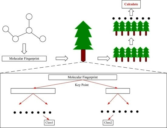
2.3. Prediction Model

Deep forests are integrated forest-based learning methods [18]. Inspired by deep learning, deep forests represent an end-to-end model where the input to the algorithm is a feature vector, which is processed in two parts: multi-grained scanning and a cascade forest. Multi-grained scanning is similar to convolutional operations in that it scans feature vectors to uncover the potential information of data, the training layer of the cascade forest is similar to DNN, and the final prediction result is similar to the softmax layer.
Multi-grained scanning is the structure of the deep forest that deals with the relationship of data features, and the most important part is the sliding window [19]. The sliding window hyperparameters are the most important of the few adjustable hyperparameters in the model. Suppose our data have D features, the sliding window size is K (which may be D/4, D/8, D/16, etc.), the step length of each slide is L (generally 1), and the number of K-dimensional feature subsample vectors P is obtained at the end of the sliding window sampling:
p = D K L + 1
And all scanned subsamples have the same label as the original sample. Next, each subsample obtained in the previous step is used as input to two random forests (including an ordinary random forest and a completely random forest), each of which outputs a class vector of length C, where C is the number of categories, and finally, the class vectors generated by the two forests are spliced to obtain the output M of this layer as:
M = 2 × D K L + 1 × C
Multi-grained scanning is shown in Figure 1.
In order to learn the relationship between feature vectors and prediction results, a cascade forest is used to process the vectors of length M derived from the multi-granularity scan to finally obtain the results. Cascade forests consist of many layers of forests, each of which includes different kinds of random forests (ordinary random forests and completely random forests), and are used to process data features layer by layer. In a cascade forest, the first layer of the forest takes the output of the multi-grained scans as input, and each subsequent layer of input is composed of stitching of the feature vectors obtained after processing in the previous layer and the original input (i.e., the input of the first layer), similar to residual connections in RESNET networks. Unlike deep learning, this process can be stopped automatically, and the stopping condition can be a hyperparameter that we set artificially, e.g., the training correct rate and the maximum number of training layers. It is also possible to verify the accuracy at each level of training when the set hyperparameters are not reached and automatically end the training when the accuracy does not improve twice in a row compared to the previous one. The output of the last layer is the classification result. At this point, the classification results of all forests are added up and averaged, and whichever category has a high proportion is output as the final result. The cascade forest is shown in Figure 2.
The random forest [20], AdaBoost [21], GBoost [22], Bayesian classifier [23], and DNN [24] models were also selected as comparison tests, where the random forest, AdaBoost, and GBoost models are also decision tree-based methods, and DNN is a deep learning method.
All machine learning models were coded and tested with the python library Scikit-learn Version 0.24.2 [25]. DNN models were coded and tested with PyTorch Version 1.10.0 [26]. All fingerprints were computed using the python library RDKit Version 2020.09.8 [27], and both ECFP4 and FCFP4 are full fingerprints of 2048 bits in length to reduce possible information loss in subsequent operations.

2.4. Evaluation Methodology

The receiver operating characteristic curve (ROC), which is frequently used to characterize a model’s performance, has two axes: the horizontal FPR (the proportion of all negative samples that are mistakenly classified as true negative samples in the positive sample category) and the vertical TPR (the proportion of all positive samples that are currently classified as true positive samples). In addition to this, we also selected accuracy, precision, and recall. Given that the goal of our work is to aid in the formation of cocrystals, precision and recall are intuitive measures of model performance. Precision is the ratio of the number of positive samples correctly classified by the classifier to the number of positive samples classified by the classifier, while recall is the ratio of the number of positive samples correctly classified by the classifier to the number of positive samples.

2.5. Febuxostat Cocrystal Screening Methodology

Cocrystal screening of febuxostat was performed using the present model to demonstrate that our model is also useful in practical applications. All candidate sample pairs were predicted using the present model. In the experiments, the synthetic model using the cooling crystallization method predicts the cocrystals that can be formed, all with a molar ratio of 1:1.
The X-ray powder diffraction spectra of cocrystals were collected on a Rigaku D/Max-2550 powder diffractometer, with CuKα (λ for Kα = 1.54059 Å) radiation at 40 kV and 250 mA. The scans were run from 3.0 to 40.0° 2θ, with an increasing step size of 0.02° and counting time duration of 1 s for each step. Data were processed using MDI-Jade version 7.0 software.
The cocrystals were characterized by single-crystal X-ray diffraction study. Single-crystal X-ray data were collected on Rigaku R-AXIS RAPID diffractometer with graphite monochromated Mo Kα (λ = 0.7107 Å) radiation at 296 K. Data reduction was performed using Crystal Structure [28,29]. A total of 4931 data points were collected, of which 3022 were unique. The crystal structure was solved with direct methods using the program SHELXS-97 and refined on F2’s anisotropic by a full-matrix, least-squares method using SHELXL-97 [30]. Anisotropic displacement parameters for non-hydrogen atoms were applied. Hydrogen atoms were placed at metrically calculated positions or the difference Fourier map and were refined isotropically using a riding mode. All C–H atoms were geometrically fixed using the command in SHELX-97, and O–H and N–H were located in difference electron density maps [30].

3. Results

3.1. Model Selection and Performance Testing

To demonstrate the advantages of the deep forest model over other models, the AUC (area under the curve in the ROC curve) of each model on top of the dataset is compared below, using a fivefold cross-validation to derive the final results. The fivefold cross-validation divides the dataset into five parts, each taking turns as a test set and the other four parts as a training set to train the model, with the final result being the average of the five experiments. In machine learning, the selection of hyperparameters plays a crucial role in the results. To eliminate the influence of hyperparameter selection on the comparison experiments, the mean value of the fivefold cross-validation is used as the criterion to find the optimal hyperparameters for each model using grid search. One of the advantages of the deep forest model is that fewer hyperparameters need to be set, so it does not take much time to find the optimal parameters. Since the molecular fingerprint is a sparse string, assuming a sliding window length of 3, many subsamples with 3D features such as {000} are scanned, which makes the training speed slow, and since the subsamples inherit the labels of the original samples, a large number of {000} subsamples with the same labels cause redundancy and reduce the accuracy. Figure 3 shows the average value of AUC for each fingerprint on all models under both encoding methods. It can be seen that the AUC value of the deep forest model is much higher than that of the other models, and the GBboost is also quite good at about 0.9. The other models are more general and all of them are in the range of 0.75 to 0.85. And the AUC values of all decision tree-based methods are greater than the rest of the models except DNN, indicating that decision tree-based methods can learn some key reasons for the formation of cocrystals.
Then, we chose a molecular fingerprint combination method (Figure 3) and found that the values of the two combination methods are similar; at this time, we used the accuracy rate for determination. The accuracy of each model is shown in Table 2, and it can be seen that except for FCFP4, the accuracy of each fingerprint splicing model is generally about 0.2% lower than the accuracy of the fingerprint summing model, so it can be excluded that it is an experimental error and the fingerprint summing model is selected as the final model.
This model is intended to assist in the formation of cocrystals, so the accuracy and regression should be as high as possible with little difference in accuracy so as not to miss any possible cocrystal formation, and the final results are shown in Table 3. In the table, it can be seen that ECFP4 has higher results than other molecular fingerprints; the accuracy is about 0.3% higher than the MACC fingerprint, about 1.2% higher than the RDKit fingerprint, and about 0.4% higher than FCFP4. For this reason, the model selects the ECFP4 fingerprint as the feature vector of the molecule.
We also note that in addition to the RF model, the GBoost model also has good performance. The cascade forest part of the deep forest model uses the random forest and completely random forest as classifiers, so we conjecture that if we replace the random forest or completely random forest classifier in the cascade forest with GBoost, it will improve the model performance, so we replaced the completely random forest in the cascade forest with the fast version of GBoost LightGBM [31]. LightGBM is in principle the same as GBoost but with improvements in processing details to speed up the training and was tested with the exam dataset and hyperparameters. The ROC curves of the random forest model, the deep forest model, and the deep forest model with the classifier set as LightGBM are shown in Figure 4 below, and the results of accuracy, precision, and regression are shown in Table 4 below. It can be seen that the deep forest model with the classifier set as LightGBM has the best results.

3.2. Case Study of Febuxostat

Febuxostat (FEB) is a very effective drug for the treatment of gout. This study uses FEB as an example simulation to illustrate that our model can guide realistic cocrystal screening. Figure 5 shows the molecules to be used in this case. In this example, it is demonstrated how our model gives predictive advice for cocrystal screening.
In general, PXRD is used to determine the crystal structure of the material to confirm whether a new crystal is formed. The model predicts that FEB and isonicotinamide, arginine, and p-aminobenzoic acid can form cocrystals. Then, experiments are carried out to synthesis FEB cocrystals. The PXRD results showed that FEB and isonicotinamide, arginine, and p-aminobenzoic acid all can form cocrystals. As shown in Figure 6, FEB–arginine cocrystal and FEB–p-aminobenzoic acid cocrystals are successfully obtained. The result of FEB–isonicotinamide cocrystal formation is consistent with our previous study [32]. In the previous work, FEB–isonicotinamide cocrystal was synthesized from acetonitrile through cooling crystallization. Its PXRD diffraction pattern is different from all the crystalline forms that have been reported for FEB and isonicotinamide (the left part in Figure 7). Then, the cocrystal was investigated by single-crystal X-ray diffraction. The results showed that the crystal was monoclinic with a space group of P 21/n. The cell parameters of the cocrystal are a = 8.2879(4) Å, b = 28.2769(10) Å, c = 9.6578(4) Å, β = 106.9430(10)°, V = 2165.12(16) Å3, and Z = 4. The formula is C16H16N2O3S·C6H6N2O. The crystal structure of FEB–isonicotinamide cocrystal is shown in Figure 7 (Right) and the molecule packing diagram of FEB–isonicotinamide cocrystal is shown in Figure 8. The crystallographic and refinement parameters for FEB–isonicotinamide cocrystal are summarized in Table 5. Crystallographic information files: CCDC no. 1479833 (https://summary.ccdc.cam.ac.uk/structure-summary?access=referee&searchdepnums=1479833&searchauthor=Yanlei, accessed on 15 May 2016).
One theory is that the deep forest model might pick up from the molecular fingerprint level that something that can alter the molecular properties is considered to be a cocrystal. Another theory is that the imbalance between positive and negative samples may even have a minor impact on the deep forest model, which is not affected by this, causing the prediction results to be biased in favor of the side with more samples, or positive samples.

4. Discussion

Combining the above results, we try to investigate the working principle of this model. Initially, it can be understood that the telomere scan end is the collection of detailed information for each sample. However, two molecules can form a cocrystal, and one can intuitively know that this is because the overall decision cannot be made by a few small parts. CNN [32] differs in that it has many fully connected layers to deal with detailed information, but the deep forest model only passes each layer’s single-digit information to the next layer, which results in poor results. For this reason, when the sliding window is selected as 3 or 4, the effect is very poor. The same can be used to explain why the predictive power is very weak when the telomere scan window is too small. This is similar to protein interaction prediction tasks where local algorithms cannot fully grasp the structure and function between proteins [33]. The effect is only improved when the window is larger. A cascade forest improves model performance by minimizing mean square error (MSE), which minimizes the sample variance of two nodes. The selected ECFP4 fingerprint effectively characterizes the molecule. This is also the reason why this model was able to achieve good performance.
So far, there have been machine learning-based, deep learning-based, and energy-based prediction models that have been successfully applied to cocrystal discovery, but our deep forest-based model still has several significant advantages.
It is well known that gathering positive and negative samples is time-consuming and laborious when using big data to build predictive models. Collecting negative samples in this work was particularly challenging because records that cannot form cocrystals are typically not purposefully recorded in the database. Although the probability of forming cocrystals is very low, some samples that can form cocrystals are inevitably marked as negative samples under such a large amount of randomly selected data, which greatly reduces the validity of the training set and, hence, the effectiveness of the model. This is not an exception to this work but a common phenomenon for which studies have been conducted to address this issue [11]. To increase the performance of the model, our model first chooses decision trees that are less sensitive to positive and negative samples. Then, it uses LightGBM as a classifier. Crucially, half of our negative samples are actually negative samples from earlier data, significantly enhancing the dataset’s validity. Therefore, our model has a good performance on the test set. Our model has advantages not only in the dataset but also in the training phase. This is because deep learning involves many hidden layers and hyperparameter tuning is very expensive. As a result, previous deep learning models frequently required advanced GPU training for several hours or weeks. Our model only needs 10 min to finish training on the i7-6700 hq in the database of approximately 1 w data because it uses the deep forest model, which reduces the need for a large number of hyperparameters and immediately ends the training when the results do not improve. This indicates that our models have a fair chance of developing further and keeping up with the times with the help of ever-increasing amounts of data in the future. They can also be taught on a home computer with minimal effort and training time. Our approach is very time-saving, especially when compared to knowledge-based prediction methods like the popular cocrystal prediction method based on molecular electrostatic potential surface measurement (MEPS) [34,35]. This method requires the calculation of the electrostatic potential of the molecule, which requires obtaining information about the molecule and putting it into the software (This contents highlighted can be deleted) for calculation. Our model takes just one computation to develop, and once built, there is no need to repeat the calculation except to enter the chemical fingerprints of the appropriate samples into the model to obtain prediction results.
In conclusion, our deep forest-based model can offer cocrystal formation predictions, save time and computing resources, and have high generalization and prediction accuracy.

5. Conclusions

In this study, a deep forest model is used to predict the outcome of cocrystal formation between molecular pairs. More than 8000 training data samples are used, of which the positive samples come from CSD. The negative samples are chosen at random using appropriate rules, and the other half are chosen from prior research and experiments to guarantee the genuine validity of the negative samples. This results in a high-quality training set that increases the model’s prediction accuracy. The testing of FEB has shown that our model can provide useful information for realistic experiments. At the same time, our model has good accuracy and fast training speed compared with the previous model, which can save a lot of computational and time resources. And as time pushes back, the CSD library will have more positive samples, papers and experiments will provide more negative samples, and the performance of the model is expected to go further. However, there are still low accuracy rates and the prediction results are biased toward positive samples due to the imbalance of positive and negative samples in the database. So, subsequent work should address how to optimize the input to solve the above problems.

Author Contributions

Conceptualization, J.C. and Y.K.; methodology, J.C.; software, J.C.; validation, Y.K. and Z.L. (Zhong Li); formal analysis, Y.K.; investigation, Y.K.; resources, Y.K.; data curation, J.C.; writing—original draft preparation, Y.K.; writing—review and editing, J.C.; visualization, Z.L. (Zhihui Li); supervision, Z.L. (Zhihui Li); project administration, Z.L. (Zhihui Li); funding acquisition, Y.K. All authors have read and agreed to the published version of the manuscript.

Funding

This work was supported by the National Natural Science Foundation of China (no. 62302165 and no. 12171434), the Science and Technology Plan Project of Huzhou City, China (no. 2022YZ03 and no. 2022GZ51), and the Postgraduate Research and Innovation Project of Huzhou University (no. 2023KYCX53).

Data Availability Statement

Program code: https://github.com/Ezrrly/FPGNet.git, accessed on 25 March 2023. The original contributions presented in the study are included in the article, further inquiries can be directed to the corresponding authors.

Acknowledgments

Thanks to all members of the research group for their support.

Conflicts of Interest

The authors declare no conflicts of interest.

References

  1. Li, J.; Wang, X.; Yu, D.; Zhoujin, Y.; Wang, K. Molecular complexes of drug combinations: A review of cocrystals, salts, coamorphous systems and amorphous solid dispersions. Int. J. Pharm. 2023, 648, 123555. [Google Scholar] [CrossRef] [PubMed]
  2. Putra, O.D.; Furuishi, T.; Yonemochi, E.; Terada, K.; Uekusa, H. Drug-drug multicomponent crystals as an effective technique to overcome weaknesses in parent drugs. Cryst. Growth Des. 2016, 16, 3577–3581. [Google Scholar] [CrossRef]
  3. Alsubaie, M.; Aljohani, M.; Erxleben, A.; McArdle, P. Cocrystal forms of the BCS class IV drug sulfamethoxazole. Cryst. Growth Des. 2018, 18, 3902–3912. [Google Scholar] [CrossRef]
  4. Barua, H.; Gunnam, A.; Yadav, B.; Nangia, A.; Shastri, N.R. An ab initio molecular dynamics method for cocrystal prediction: Validation of the approach. CrystEngComm 2019, 21, 7233–7248. [Google Scholar] [CrossRef]
  5. Hollingsworth, S.A.; Dror, R.O. Molecular dynamics simulation for all. Neuron 2018, 99, 1129–1143. [Google Scholar] [CrossRef] [PubMed]
  6. Balmohammadi, Y.; Grabowsky, S. Arsenic-Involving Intermolecular Interactions in Crystal Structures: The Dualistic Behavior of As (III) as Electron-Pair Donor and Acceptor. Cryst. Growth Des. 2023, 23, 1033–1048. [Google Scholar] [CrossRef]
  7. Grecu, T.; Hunter, C.A.; Gardiner, E.J.; McCabe, J.F. Validation of a computational cocrystal prediction tool: Comparison of virtual and experimental cocrystal screening results. Cryst. Growth Des. 2014, 14, 165–171. [Google Scholar] [CrossRef]
  8. Ryan, K.; Lengyel, J.; Shatruk, M. Crystal structure prediction via deep learning. J. Am. Chem. Soc. 2018, 140, 10158–10168. [Google Scholar] [CrossRef]
  9. Wicker, J.G.P.; Crowley, L.M.; Robshaw, O.; Little, E.J.; Stokes, S.P.; Cooper, R.I.; Lawrence, S.E. Will they co-crystallize? CrystEngComm 2017, 19, 5336–5340. [Google Scholar] [CrossRef]
  10. Wang, D.; Yang, Z.; Zhu, B.; Mei, X.; Luo, X. Machine-Learning-Guided Cocrystal Prediction Based on Large Data Base. Cryst. Growth Des. 2020, 20, 6610–6621. [Google Scholar] [CrossRef]
  11. Devogelaer, J.J.; Meekes, H.; Tinnemans, P.; Vlieg, E.; de Gelder, R. Co-crystal prediction by artificial neural networks. Angew. Chem. Int. Ed. 2020, 59, 21711–21718. [Google Scholar] [CrossRef]
  12. Zhou, Z.H.; Feng, J. Deep forest. Natl. Sci. Rev. 2019, 6, 74–86. [Google Scholar] [CrossRef] [PubMed]
  13. Allen, F.H.; Taylor, R. Research applications of the Cambridge structural database (CSD). Chem. Soc. Rev. 2004, 33, 463–475. [Google Scholar] [CrossRef] [PubMed]
  14. Devogelaer, J.-J.; Brugman, S.J.T.; Meekes, H.; Tinnemans, P.; Vlieg, E.; de Gelder, R. Cocrystal design by network-based link prediction. CrystEngComm 2019, 21, 6875–6885. [Google Scholar] [CrossRef]
  15. Liu, H.; Sun, J.; Guan, J.; Zheng, J.; Zhou, S. Improving compound–protein interaction prediction by building up highly credible negative samples. Bioinformatics 2015, 31, i221–i229. [Google Scholar] [CrossRef] [PubMed]
  16. Ferrence, G.M.; Tovee, C.A.; Holgate, S.J.; Johnson, N.T.; Lightfoot, M.P.; Nowakowska-Orzechowska, K.L.; Ward, S.C. CSD Communications of the Cambridge Structural Database. IUCrJ 2023, 10, 6–15. [Google Scholar] [CrossRef] [PubMed]
  17. Bennion, J.C.; Matzger, A.J. Development and evolution of energetic cocrystals. Acc. Chem. Res. 2021, 54, 1699–1710. [Google Scholar] [CrossRef] [PubMed]
  18. Xu, X.; Chen, T.; Minami, M. Intelligent fault prediction system based on internet of things. Comput. Math. Appl. 2012, 64, 833–839. [Google Scholar] [CrossRef]
  19. Tao, Y.; Papadias, D. Maintaining sliding window skylines on data streams. IEEE Trans. Knowl. Data Eng. 2006, 18, 377–391. [Google Scholar]
  20. Breiman, L. Random forests. Mach. Learn. 2001, 45, 5–32. [Google Scholar] [CrossRef]
  21. Rätsch, G.; Onoda, T.; Müller, K.R. Soft margins for AdaBoost. Mach. Learn. 2001, 42, 287–320. [Google Scholar] [CrossRef]
  22. Friedman, J.H. Greedy function approximation: A gradient boosting machine. Ann. Stat. 2001, 29, 1189–1232. [Google Scholar] [CrossRef]
  23. Chebil, W.; Wedyan, M.; Alazab, M.; Alturki, R.; Elshaweesh, O. Improving Semantic Information Retrieval Using Multinomial Naive Bayes Classifier and Bayesian Networks. Information 2023, 14, 272. [Google Scholar] [CrossRef]
  24. LeCun, Y.; Bengio, Y.; Hinton, G. Deep learning. Nature 2015, 521, 436–444. [Google Scholar] [CrossRef] [PubMed]
  25. Pedregosa, F.; Varoquaux, G.; Gramfort, A.; Michel, V.; Thirion, B.; Grisel, O.; Blondel, M.; Prettenhofer, P.; Weiss, R.; Dubourg, V.; et al. Scikit-learn: Machine learning in Python. J. Mach. Learn. Res. 2011, 12, 2825–2830. [Google Scholar]
  26. Paszke, A.; Gross, S.; Massa, F.; Lerer, A.; Bradbury, J.; Chanan, G.; Killeen, T.; Lin, Z.; Gimelshein, N.; Antiga, L.; et al. Pytorch: An imperative style, high-performance deep learning library. In Advances in Neural Information Processing Systems 32 (NeurIPS 2019), Proceedings of the 33rd International Conference on Neural Information Processing Systems, Vancouver, BC, Canada, 8–14 December 2019; Curran Associates Inc.: Red Hook, NY, USA, 2019. [Google Scholar]
  27. Landrum, G. RDKit: A software suite for cheminformatics, computational chemistry, and predictive modeling. Greg Landrum 2013, 8, 31. [Google Scholar]
  28. Rigaku. PROCESS-AUTO; Rigaku Corporation: Tokyo, Japan, 1998. [Google Scholar]
  29. Rigaku. CrystalStructure; Version 3.8.0; Rigaku Corporation: Tokyo, Japan; Rigaku Americas: The Woodlands, TX, USA, 2007. [Google Scholar]
  30. Sheldrick, G.M. A short history of SHELX. Acta Crystallogr. A 2008, 64, 112–122. [Google Scholar] [CrossRef]
  31. Ke, G.; Meng, Q.; Finley, T.; Wang, T.; Chen, W.; Ma, W.; Ye, Q.; Liu, T.-Y. Lightgbm: A highly efficient gradient boosting decision tree. In Advances in Neural Information Processing Systems 30 (NIPS 2017), Proceedings of the 31st International Conference on Neural Information Processing Systems, Long Beach, CA, USA, 4–9 December 2017; Curran Associates Inc.: Red Hook, NY, USA, 2017. [Google Scholar]
  32. Kang, Y.; Gu, J.; Hu, X. Syntheses, structure characterization and dissolution of two novel cocrystals of febuxostat. J. Mol. Struct. 2017, 1130, 480–486. [Google Scholar] [CrossRef]
  33. Shin, H.C.; Roth, H.R.; Gao, M.; Lu, L.; Xu, Z.; Nogues, I.; Yao, J.; Mollura, D.; Summers, R.M. Deep convolutional neural networks for computer-aided detection: CNN architectures, dataset characteristics and transfer learning. IEEE Trans. Med. Imaging 2016, 35, 1285–1298. [Google Scholar] [CrossRef]
  34. Kovács, I.A.; Luck, K.; Spirohn, K.; Wang, Y.; Pollis, C.; Schlabach, S.; Bian, W.; Kim, D.-K.; Kishore, N.; Hao, T.; et al. Network-based prediction of protein interactions. Nat. Commun. 2019, 10, 1240. [Google Scholar] [CrossRef]
  35. Chalkha, M.; El Hassani, A.A.; Nakkabi, A.; Tüzün, B.; Bakhouch, M.; Benjelloun, A.T.; Sfaira, M.; Saadi, M.; El Ammari, L.; El Yazidi, M. Crystal structure, Hirshfeld surface and DFT computations, along with molecular docking investigations of a new pyrazole as a tyrosine kinase inhibitor. J. Mol. Struct. 2023, 1273, 134255. [Google Scholar] [CrossRef]
Figure 1. Multi-grained scanning: n is the sample length, s is the window length, and l is the step size.
Crystals 14 00313 g001
Figure 2. Schematic diagram of the computational process of cascade forest.
Crystals 14 00313 g002
Figure 3. Statistical results of ROC values of different models on different molecular fingerprints.
Crystals 14 00313 g003
Figure 4. ROC curves of the three models.
Crystals 14 00313 g004
Figure 5. Molecular structure diagram of the subject molecule and guest molecules (the first is the subject molecule; the rest are the guest molecules. The molecules predicted by the model that can form crystals are in the green box, and the cocrystal results obtained in this experiment are in the checked box, ✓ represents the guest molecule that has been experimentally demonstrated to form cocrystal with Entecavir).
Crystals 14 00313 g005
Figure 6. (Left): comparison of the X-ray powder diffraction patterns of the FEB–arginine cocrystal (a), arginine (b), and febuxostat (c). (Right): comparison of the X-ray powder diffraction patterns of the FEB–p-aminobenzoic acid cocrystal (a), p-aminobenzoic acid (b), and febuxostat (c).
Crystals 14 00313 g006
Figure 7. (Left): comparison of the X-ray powder diffraction patterns of the FEB–isonicotinamide cocrystal (a), isonicotinamide (b), and febuxostat (c). (Right): crystal structure of FEB–isonicotinamide cocrystal (carbon atom: grey, oxygen atom: red, hydrogen atom: white, nitrogen atom: blue, sulfur atom: yellow).
Crystals 14 00313 g007
Figure 8. Molecular arrangement for FEB–isonicotinamide cocrystal.
Crystals 14 00313 g008
Table 1. Information about molecular fingerprints.
Information about Molecular FingerprintsLength (Bits)Emphasis
MACCS166substructure
RDKit2048molecular structure
ECFP42048atomic radius
FCFP42048atomic properties
Table 2. The accuracy of the combination of two molecular fingerprints in the model.
Fingerprint TypeAccuracy
MACCS add95.26%
MACCS connect94.92%
RDKit add94.19%
RDKit connect94.03%
ECFP4 add95.51%
ECFP4 connect95.35%
FCFP4 add95.16%
FCFP4 connect94.24%
Table 3. Accuracy, precision, and recall of different molecular fingerprints.
ECFP4FCFP4MACCSRDKit
Accuracy95.51%95.16%95.26%94.19%
Precision94.03%94.42%94.55%94.21%
Recall95.75%95.26%93.23%95.09%
Sensitivity97.82%97.46%97.57%96.83%
Specificity95.26%95.31%95.14%95.13%
Average95.67%95.52%95.15%95.09%
Table 4. Accuracy, precision, and recall of the models.
RFDeep ForestDeep Forest (LightGBM)
Accuracy82.93%95.51%96.15%
Precision82.41%94.03%94.85%
Recall83.96%95.75%96.69%
Sensitivity92.52%97.82%97.91%
Specificity72.76%95.26%95.83%
Table 5. Selected crystallographic and refinement parameters for FEB–isonicotinamide cocrystal structures.
Empirical FormulaC16H16N2O3S ▪ C6H6N2OX-ray Wavelength0.71073 Å
Formula weight438.49Range h−10 to 10
Crystal systemMonoclinicRange k−36 to 36
Space groupP 21/nRange l−12 to 12
T (K)296(2)Reflections collected12,542
a (Å)8.2879(4)Total reflections4931
b (Å)28.2769(10)Observed reflections3022
c (Å)9.6578(4)R[I > 2σ(I)]0.0948
α (°)90(∆/σ) max0.000
β (°)106.943S1.011
γ (°)90Rint0.0607
V (Å3)2165.12wR (F2)0.1304
θ range3.1–27.5Goodness of fit1.011
Z4DiffractometerRigaku RAXIS-RAPID
Crystal size (mm)0.43 × 0.23 × 0.18Refinement methodfull-matrix least-squares on F2
Disclaimer/Publisher’s Note: The statements, opinions and data contained in all publications are solely those of the individual author(s) and contributor(s) and not of MDPI and/or the editor(s). MDPI and/or the editor(s) disclaim responsibility for any injury to people or property resulting from any ideas, methods, instructions or products referred to in the content.

