Article

Phase-Only Liquid-Crystal-on-Silicon Spatial-Light-Modulator Uniformity Measurement with Improved Classical Polarimetric Method

School of Electronic Science and Engineering, Southeast University, Nanjing 210096, China
*
Author to whom correspondence should be addressed.
Crystals 2023, 13(6), 958; https://doi.org/10.3390/cryst13060958
Submission received: 18 May 2023 / Revised: 5 June 2023 / Accepted: 7 June 2023 / Published: 15 June 2023
(This article belongs to the Special Issue Advances in Liquid Crystal Optical Devices)

Abstract

:
The classical polarimetric method has been widely used in liquid crystal on silicon (LCoS) phase measurement with a simple optical setup. However, due to interference caused by LCoS cover glass reflections, the method lacks accuracy for phase uniformity measurements. This paper is aimed at mathematically analyzing the errors caused by non-ideal glass reflections and proposing procedures to reduce or eliminate such errors. The measurement is discussed in three conditions, including the ideal condition with no reflections from the LCoS cover glass, the condition with only the front reflection from the cover glass, and the condition with only the back reflection from the cover glass. It is discovered that the backward reflection makes the largest contribution to the overall measurement error, and it is the main obstacle to high-quality measurements. Several procedures, including optical alignment, LC layer thickness measurement, and phase estimation method, are proposed, making the uniformity measurement more qualitative and consistent.

1. Introduction

Liquid crystal on silicon spatial light modulators (LCoS-SLMs) are devices used to perform spatial modulation of the light wavefront, and they have been commonly used in a wide range of applications, including holographic displays and others [1]. Phase-only LCoS-SLM requires an accurate spatial phase response, which describes the phase uniformities and linearity across the whole active area [1,2,3].
Multiple research groups [4,5,6] have presented interferometry methods to measure and calibrate the reflected wavefront from LCoS-SLMs, and such methods have become the preferred choice for measuring the LCoS phase uniformity whenever available. Figure 1 shows one of the possible optical setups for the interferometry measurement of the LCoS wavefront [5]. However, due to the nature of interferometry, these methods usually require a highly stable environment with minimal vibration and ambient light [7,8,9], which is not always available in every circumstance.
In this paper, we evaluated the classical polarimetric method [10,11,12,13] to validate its application in the measurement of the non-uniform phase response of LCoS-SLMs. The method can measure the absolute phase retardation and phase flicker at any region of the active area, while it only requires basic equipment, as demonstrated in Figure 2, as well as a normal lab test environment without ambient light controlling. The classical polarimetric method is an indirect measurement of phase retardation. It measures the relation between output light intensity I and input gray level G L , and it calculates phase retardation Γ based on normalized intensity I n o r m . Such a setup is not sensitive to vibrations, and by measuring the normalized light intensity in the output, the effect of ambient light is mostly eliminated.
The measuring process divides the whole active area of the tested LCoS device into a grid of regions, and in each region, the classical polarimetric method is performed to acquire its phase response [13]. A two-axis linear translation stage is used to traverse all regions. By combining the results from all regions, a distribution of the phase response could be calculated. Additionally, to ensure consistent measurements, the LCoS device was also kept at a stable temperature during the whole process.
However, there are some disagreements between ideal conditions in theory and actual test environments in practice, especially when anti-reflection (AR) coating is not present. Figure 3a shows an actual uniformity measurement from one of our LCoS devices with the setup shown in Figure 2, and the rippled result is clearly not what could be expected in an LCoS assembly [14,15], and it does not provide a solid foundation for the calibration process.
During this experiment, we found that the pattern appearing in the phase result shared close similarity with the interference pattern observed on the LCoS device, shown in Figure 3b. According to this outcome, we were investigating a relationship between the error pattern and the reflections on the cover glass of the LCoS device with analytical modeling and simulation and comparing them with more detailed experiments.
Our work is aimed at analyzing and addressing the error caused by glass reflections to make the polarimetric method a more viable means for LCoS phase uniformity measurement. By considering the glass reflections and choosing unaffected data points, our improved measuring method could better compensate for the error caused by glass reflections, thus achieving a more accurate phase uniformity measurement compared to the original classical polarimetric method.

2. Materials and Methods

The polarimetric method used in this paper is based on the work by Márquez, A. et.al. [10,11], which used a single collimated laser beam passing through polarizer P1, LCoS (as a waveplate), and polarizer P2 in order, and it calculated the phase retardation by measuring the transmitted laser intensity. The basic principle of the polarimetric method is demonstrated in Figure 4, with the slow axis of the waveplate defined as the X-axis.

2.1. Basic Polarimetric Method

To obtain the relationship between the phase retardation of the LCoS device and the transmitted light intensity, some theoretical development is needed. The detailed derivation process with Jones calculus under ideal condition can be found at [10,11]. This sub-section only discusses the parameter definitions and the final conclusion as a foundation for later analysis.
First, the induced phase difference of ordinary light and extraordinary light after passing through the LCoS device are marked as φ o and φ e f f , which correspond to their optical path lengths (OPLs) respectively. The liquid crystal (LC) is assumed to be a positive birefringence material, where φ e f f > φ o is always true.
The formulas below define φ o , φ e f f , and phase retardation Γ , where n o λ and n e f f λ are the effective refractive indices of LC material at the wavelength λ , and d is the distance that light travels through the liquid crystal, which is double the thickness of the LC layer in this LCoS device. Tilting of the LC molecule is considered in n e f f λ , which indicates the effective refractive index on the slow axis of the LCoS device.
φ o = 2 π n o λ d λ
φ e f f = 2 π n e f f λ d λ
Γ = φ e f f φ o = 2 π ( n e f f λ n o λ ) d λ
For the simplicity of the calculation, the orientation of the slow axis of the LCoS device, which is the polarization orientation of the extraordinary light, is defined as the X axis. The Jones matrix of the LCoS device W φ e f f , φ o can be written as follows:
W φ e f f , φ o = e i φ e f f 0 0 e i φ o
At the same time, the Jones matrix of the polarizer P θ can be written as follows, where θ is the angle between its transmissive axis and X-axis defined above.
P θ = c o s 2 θ c o s θ s i n θ c o s θ s i n θ s i n 2 θ ,       θ π 2 , π 2
For the simplicity of the calculation again, the light intensity of the laser beam after polarizer P1 is marked as I i n . When θ 1 and θ 2 are orthogonal to each other, which means θ 1 θ 2 = ± π 2 , I o u t can be calculated as:
I o u t = I i n 2 s i n 2 2 θ 1 1 c o s Γ
As can be seen, I o u t can always be normalized into I n o r m , which is only related to phase retardation Γ . As a result, Γ can be calculated from normalized light intensity I n o r m during measurement:
I n o r m = 1 2 1 c o s Γ
Γ = a c o s 1 2 I n o r m
Under ideal conditions in which the reflection from the LCoS cover glass is ignored, and all optical components, including the laser beam and polarizers, are perfectly aligned, the measurement is guaranteed to be error-free.

2.2. Reflections on the LCoS Cover Glass

All the discussion and math formulas in Section 2.1 are based on an ideal modeling of the optical system. It is assumed that all the incident light is modulated by the LC layer exactly twice, including once inward and once outward. However, this case usually does not apply in real-life practice.
In practice, part of the incident light would be reflected without modulation from the LC layer, while part of the remaining light can be modulated multiple times [16]. Such un-modulated or over-modulated reflection mainly comes from the surface reflection of the cover glass, and the intensity of this reflection is usually around 8% on an uncoated air-glass-air surface, and somewhere between 4% and 8% on an air-glass-LC surface [17,18]. Figure 5 considers three different reflection paths in the LCoS device as the example, with no modulation, normal modulation, and double modulation, respectively.
The corresponding waveplates in each case are marked as W 0 , W 1 , and W 2 , and their respective Jones matrices are shown as below. The mirroring effect caused by reflection is ignored since, in every case, the reflection count is an odd number.
W 0 φ e f f , φ o = 1 0 0 1
W 1 φ e f f , φ o = e i φ e f f 0 0 e i φ o
W 2 φ e f f , φ o = e i 2 φ e f f 0 0 e i 2 φ o
To model the glass reflection of the LCoS device, transmittance and reflectivity of the cover glass are defined. To simplify the model, the glass thickness is ignored, and reflections from all surfaces of the cover glass are treated as a single surface reflection, as the coherent length of laser in this experiment can be treated as infinite compared to the thickness of the cover glass. As a result, the single surface reflectivity is equal to the combined interference result of all the separated surfaces and its phase as a reference zero point. The glass absorption is ignored in all cases.
When the light is traveling from air toward LC (air-glass-LC), the transmittance of the cover glass is marked as A and the reflectivity as 1 A . With the same principle, when the light is traveling from LC toward air (LC-glass-air), the transmittance of the cover glass is marked as B and the reflectivity as 1 B . These two reflections are named front reflection (case W 0 in Figure 5) and back reflection (case W 2 in Figure 5) for simplicity. To simplify the expressions, A and B can be rewritten as:
A = c o s 2 α ,     1 A = s i n 2 α
B = c o s 2 β ,     1 B = s i n 2 β
These non-ideal reflections in W 0 and W 2 could cause systematic errors in the phase measurement of actual LCoS devices, with their principles illustrated in Appendix A. Such errors are further discussed with mathematical derivation and simulated experiments in subsequent subsections.
Simulations in the following sections are based on an 8-bit vertical-aligned (VA) LCoS device with an average LC layer thickness of 6   μ m ,and LC material with a refractive index of n o = 1.49 and n e = 1.60 . Both front and back reflectivity were set to 5 % unless specified otherwise, and a collimated 635   n m laser source with infinite coherence length was used. The non-uniform LC layer thickness was simulated by a spherical CMOS backplane with a curvature of 100   m , giving a peak–peak difference of 478   n m across its 12.3   m m × 6.9   m m active area. The thickness and non-uniformity of the LC layer were slightly amplified compared to a more common thickness of 3   μ m and peak–peak difference of 100   n m [14] to emphasize the effect of glass reflection.

2.3. Theory and Analysis with Un-Modulated Front Reflection

In this subsection, only the front reflection of the cover glass is considered, which means that only W 0 and W 1 are included. W 2 is temporarily ignored in this subsection for simplicity reasons.
The Jones matrix of the LCoS device should be rewritten as:
W φ e f f , φ o , α = c o s α W 1 φ e f f , φ o + s i n α W 0 φ e f f , φ o                                     = e i φ e f f c o s α + s i n α 0 0 e i φ o c o s α + s i n α
Further, the complex amplitude of the transmitted light can be calculated with
E o u t = P θ 2 W φ e f f , φ o , α I i n c o s θ 1 s i n θ 1
The transmitted light intensity I o u t changes into the following form:
I o u t = I i n e i Γ c o s θ 1 c o s θ 2 + s i n θ 1 s i n θ 2 e i φ o c o s α + c o s θ 1 θ 2 s i n α 2
Note the newly appeared term c o s θ 1 θ 2 s i n α on the right side. Apparently, either when the orthogonal relation between θ 1 and θ 2 is satisfied or the reflectivity s i n 2 α equals to zero, the above expression would degenerate into the form obtained in Section 2.1, and the calculation should be error-free under this circumstance. This outcome is understandable, as the reflected component from W 0 has the same polarization state as polarizer P1 and should be filtered out by the second polarizer P2.
For example, when θ 1 and θ 2 are orthogonal to each other, and the transmittance of the cover glass A = c o s 2 α is less than 1, I o u t can be expressed as follows:
I o u t = I i n 2 c o s 2 ( α ) s i n 2 2 θ 1 1 c o s Γ
However, in cases in which θ 1 and θ 2 are not orthogonal, and transmittance A is less than 1, the light intensity I o u t cannot be transformed into a simple form. In this case, the final output intensity is not only related to the phase retardation Γ but also related to the optical path difference φ o , and it is no longer possible to calculate the phase retardation Γ with normalized output intensity I n o r m .
Considering that the reflectivity of the LCoS device is usually not controllable during the measurement, the proper alignment of the polarization orientation can be very important in this scenario. One possible source of such misalignment is the non-polarizing beam splitter (NPBS) used in this setup, which can bring up to 10 ° of polarization angle change and a certain amount of linearity degradation [19]. A possible solution to this problem is further discussed in Appendix A.

2.4. Theory and Analysis with Double-Modulated Back Reflection

In this case, only the back reflection of the cover glass is considered, which means only W 1 and W 2 are included, and W 0 is assumed to have been already corrected by the orthogonal polarizer pair, which means θ 1 θ 2 = ± π 2 is already satisfied, and light from the front reflection will not pass through the second polarizer P2. W 0 is ignored in the math derivations but still included in the simulations. Note that W 0 is ignorable only when P2 is orthogonal to P1 in this measuring process, which is not the case when LCoS is used in actual applications, such as holographic displays or wavelength selective switches, in which only extraordinary light is present [20,21].
The Jones matrix of the LCoS device should be rewritten as:
W φ e f f , φ o , β = c o s β W 1 φ e f f , φ o + s i n β W 2 φ e f f , φ o                                                                             = e i φ e f f c o s β + e i 2 φ e f f s i n β 0 0 e i φ o c o s β + e i 2 φ o s i n β
Moreover, the transmitted light can be calculated as:
E o u t = P θ 2 W φ e f f , φ o , β I i n c o s θ 1 s i n θ 1
By applying the above assumed θ 1 θ 2 = ± π 2 , the expressions for transmitted light intensity can be simplified into:
I o u t = 1 4 s i n 2 2 θ 1 I i n e i Γ 1 e i φ o c o s β + e i 2 Γ 1 e i 2 φ o s i n β 2
As can be seen, only if the reflectivity s i n 2 β equals zero does the above expression for I o u t degenerate into the form of I o u t in Equation (6), and it can be normalized into I n o r m = 1 c o s Γ / 2 . However, when the reflectivity cannot be ignored, I o u t Γ relation is additionally affected by the changing interference caused by double-modulation, and no longer follows the ideal sine-wave shape. Only when the phase retardation satisfies Γ = 2 k π , k Z can the distorted I o u t agree with its undistorted form I o u t at its minimum value point. This finding indicates that only phase at Γ = 2 k π , k Z can be correctly measured. Note that, when Γ = 2 k + 1 π , k Z , although the form of I o u t agrees with I o u t , it does not reach its maximum value due to the constructive interference next to this location, and the actual phase cannot be calculated at this point.
Figure 6a shows a simulation of the relation between I o u t and input gray level (GL) in one of the regions, while Figure 6b shows the change in average and peak–peak measurement error across the whole active area. An obvious relation between error and I o u t can be seen, that is, when I o u t reaches its minimum value, the measurement error also reaches its minimum, and the average phase can be viewed as error-free. This discovery is critical for the uniformity retrieving method discussed in the next subsection, which allows for uniformity calculation based on these error-free points at Γ = 2 π .
Note that the average measurement error across the active area is related to the LC layer thickness non-uniformity such that, when the thickness non-uniformity is greater, both positive error and negative error would appear and cancel each other out in the average value, while when the thickness non-uniformity is smaller, positive and negative errors are less likely to be balanced, and the average error would be greater and closer to the peak error.

2.5. Retrieving LCoS Uniformity from the Data Affected by Back Reflection

To address this error caused by back reflection and to obtain the correct uniformity data, the known error-free point at Γ = 2 k π ,   k Z can be utilized. Since the average phase result at this point can also be viewed as error-free, it is possible to retrieve the actual phase uniformity based on this set of data, assuming that the non-uniformity of phase response is solely determined by the non-uniformity of LC layer thickness. Additionally, in case the LC refractive indices n o λ and n e λ are known, and the maximum phase retardation can be reached at maximum G L , the uniformity of φ o and the LC layer thickness could also be calculated. Figure 7 demonstrates the basic principle of this process with simulation data obtained in Section 2.4.
For each measured region, we first find the designated low point where I o u t reaches its minimum value, and the phase retardation is 2 π . We mark the gray level at this point as G L 2 π . This low point should be the closest one to the zero phase retardation point, which should be the first low point after zero driving voltage for a common vertical-aligned LCoS (VA-LCoS) and the last low point before max driving voltage for common parallel-aligned LCoS (PA-LCoS) [22].
Then, we find the average measured phase of the whole active area at the max phase retardation point as Γ ¯ m a x , and the average measured phase across the whole active area at G L 2 π as Γ ¯ G L 2 π . Note that both Γ ¯ m a x and Γ ¯ G L 2 π are calculated from the original faulty result. The full phase retardation in this region can be approximately calculated as follows, assuming that the average error of the phase measurement at G L 2 π is much smaller than the peak error, as demonstrated in Figure 6b.
Γ m a x = 2 π Γ ¯ m a x / Γ ¯ G L 2 π
Since we have assumed that the phase retardation is only related to LC layer thickness, the thickness can be calculated by multiplying phase retardation by λ / 2 π n o λ , and the final expression of LC layer thickness d / 2 at this location can be written as:
d / 2 1 2 Γ ¯ m a x Γ ¯ G L 2 π λ n e λ n o λ
Repeating such processes for all regions of the LCoS active area, we can then acquire a uniformity map of the LC layer thickness on this LCoS device.

3. Results

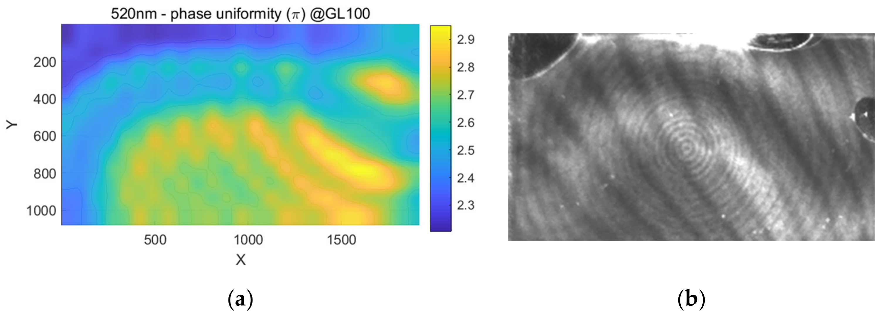
3.1. Results of the Front Reflection

According to the theory and modeling in Section 2.3, a simulated measurement when the second polarizer P2 is misaligned by 10 degrees is calculated, as demonstrated in Figure 8. Ripple-shaped measurement error can be seen in the result.
Figure 9 shows the result of a measured phase uniformity on an LCoS device. The polarization orientation was properly aligned in Figure 9a, while Figure 9b presents the result when the orientation was misaligned by 8 degrees due to NPBS distortion. Similar patterns could be seen compared to the simulated result in Figure 8, and the amplitude of measurement error was also in line with the simulation. However, since the amplitude of this error caused by the front reflection was very small (usually less than ± 0.02 π ), it could easily be confused with other noises in the measurement process, especially when the phase flicker was large. The conclusion by Martínez et al. in their demonstration of the classical polarimetric method, stating that high quality NPBS does not present a considerable difference in LCoS phase measurement [11], can be confirmed according to our simulations and experiments.

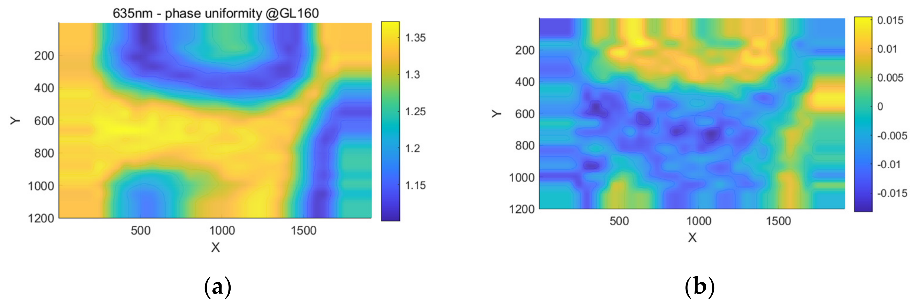
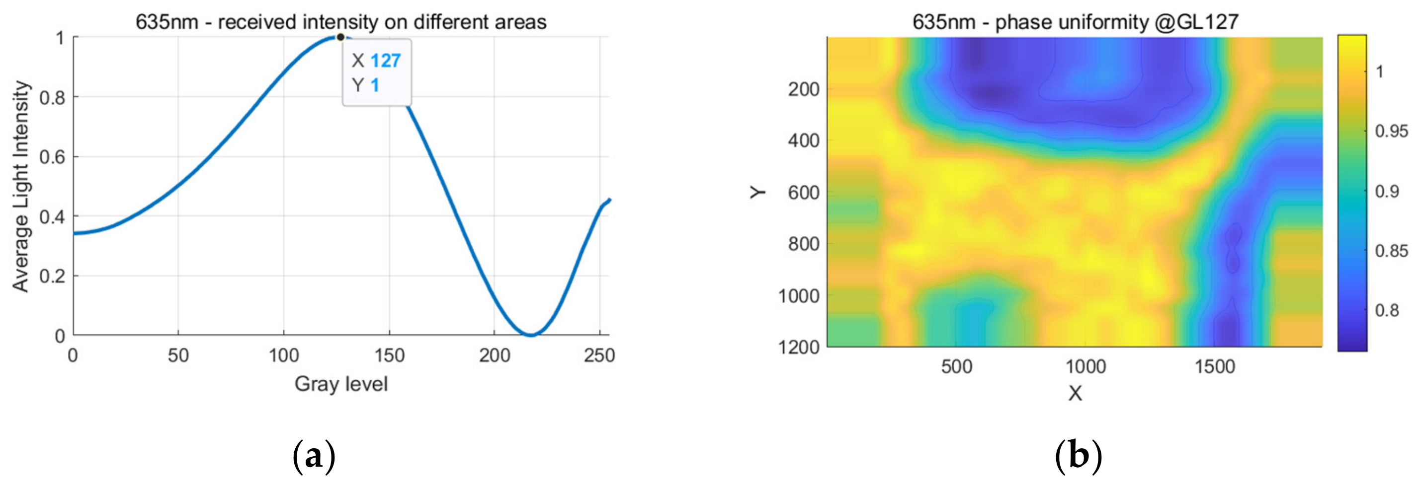
3.2. Results of the Back Reflection

As discussed and analyzed in Section 2.4, the results when back reflection is present should be discussed in two separate parts, with one part focusing the gray level where maximum error occurs, and another part focusing the gray level where only minimum error occurs.
Figure 10 demonstrates the simulated worst-case scenario, when I o u t and the measurement error are at the maximum, as indicated in Figure 10a. Compared to the real phase in Figure 10b, the measured phase distribution in Figure 10c shows a clear ripple-shaped error pattern, and the phase error can reach up to ± 0.25 π , as demonstrated in Figure 10d, completely invalidating the measurement result. The error pattern shows a clear periodical relation with the LC layer thickness, resulting in a rippled shape.
Notice that the max amplitude of such a phase measurement error has a positive relationship with the reflectivity of the cover glass. According to the simulation, when the reflectivity is 1%, the maximum measurement error is around ± 0.12 π , which is lower than that from a 5% reflection.
Meanwhile, Figure 11 demonstrates the simulated best-case scenario when I o u t and the measurement error are at the minimum, as indicated in Figure 11a. Compared to the real phase in Figure 11b, the measured phase distribution in Figure 11c shows only very little measurement error, which is around ± 0.025 π .
The phase error across the whole active area never reaches zero, as shown in Figure 6b, since the non-uniformity of the LC layer indicates that different areas would reach their error-free point of Γ = 2 k π , k Z at different input gray levels, and there will always be some area with measurement error regardless of the gray level used.
The effect of the back reflection in an actual real-life measurement is compared to the simulation and analyzed in subsequent paragraphs. According to the discussion in Section 2.4, when the measured light intensity is around its maximum value, the phase measurement error also reaches its maximum. Figure 12 demonstrates the measured intensity-GL relationship (Figure 12a) and the calculated phase distribution (Figure 12) at the indicated GL127 input. As shown in the figure, the amplitude of this ripple-shaped pattern is about ± 0.15 π , in line with the simulated results in Section 2.4 and Figure 10. This error cannot be ignored in the phase uniformity measurement.
Figure 13 demonstrates the measured intensity–GL relationship (Figure 13a) and the calculated phase distribution (Figure 13b) at the indicated GL212 input. The amplitude of the error pattern is only around ± 0.02 π in this condition, which also agrees with the simulated result in Figure 11.
By comparing the shape and amplitude of such ripple-shaped patterns under different GL inputs, the results of our experiment match the theory in Section 2 quite well, indicating that the theory is effective and can be used to guide the LCoS uniformity retrieving process.

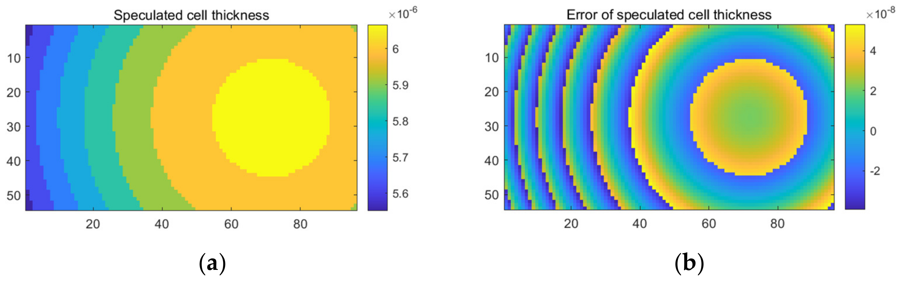
3.3. Results of the LCoS Uniformity Retrieving

Figure 14 demonstrates a simulation of our uniformity retrieving process, assuming the birefringence refractive index is accurate, and the max phase retardation is reached at G L = 255 . Figure 14a shows the speculated LC layer thickness based on measured light intensity I o u t , and the error of such speculation is less than 1%, as shown in Figure 14b.
One main source of the error is the discrete gray level control, which makes it impossible to locate the exact low point between two neighboring gray levels, where I o u t reaches its minimum. The other main source of error is the difference between the average measured phase and the actual phase, as demonstrated in Figure 6b. Additionally, the discrete gray level addressed also makes the resolution of this uniformity result relatively low, as can be seen in Figure 14a with discrete steps.
This simulation indicates that it is actually a viable option for roughly measuring the uniformity of LC layer thickness on LCoS devices, with the drawback of having to measure the full modulation range of the LCoS device and having to know the exact refractive indices of the LC material. However, if the absolute value of the thickness is not needed, both the full modulation range and the exact LC refractive indices are no longer required. The relative uniformity can still be obtained by only measuring a single full 2 π phase range of the whole active area. In this case, only the relative relation in the calculated uniformity map holds true.
For the actual measured data in real-life experiments, the LC thickness uniformity can be obtained based on Equation (22). Figure 15a shows the calculated LC layer thickness of this LCoS device indexed by subregions, and a clear saddle-shaped pattern can be seen. By comparing it to the interference pattern obtained on the same LCoS device shown in Figure 15b, obvious similarities can be seen, and the calculated thickness difference also matches the number of interference stripes, indicating the effectiveness of this method, which extracts the uniformity of the LCoS device.
The pattern and peak–peak difference in this calculated LC layer thickness also agrees with the common saddle-shaped cell gap thickness pattern on LCoS devices demonstrated in other research groups’ work [14], indicating that this process is indeed effective at phase around 2 k π ,   k Z .
It is also worth mentioning that, if the LC refractive index is inaccurate, or the max phase retardation is not reached, the absolute value of this thickness speculation will also be inaccurate as a linear scale of the real value. However, even in this case, the relative uniformity is still preserved.

4. Discussion

The LC thickness uniformity of our LCoS device has been calculated in Section 3, but the linearity of the phase response Γ is still not fully obtained. According to Equation (20), if φ o is accurately measured, the phase retardation Γ can be calculated. However, in our simulation setup, with an average LC layer thickness of 6   μ m and n o = 1.49 at 635   n m , the average value of the total ordinary phase φ o is around 55 π , which means the accuracy of measured φ o is only about 0.5 π , not including other possible errors caused by inaccurate refractive indices or driving strength. Such accuracy is not enough to calculate phase retardation Γ based on I o u t in Equation (20), which requires E r r φ o π . Therefore, an accurate result of Γ was not yet achievable in this setup.
On the other hand, since the relative uniformity of the LC layer thickness is known, the uniformity of phase retardation can still be hypothesized based on this calculated data, assuming that the phase response is only determined by the LC layer thickness and driving voltage, ignoring all other possible non-uniform aspects.
First, calculate the phase of reflected ordinary light based on the measured LC layer thickness d / 2 . The uniformity distribution of the property (e.g., φ , d or Γ ) is marked in bold to differentiate from that the measured value from a single point. The result in this step might not be accurate, but it should be proportional to the real value.
φ o = 2 π n o λ d λ
Then, for each gray level GL, assume the distribution of phase retardation Γ is proportion to the distribution of ordinary phase difference φ o , which means Γ = k φ o . The least square method can be used to determine the coefficient value k , causing the speculated Γ to match the measured Γ in the experiment. Repeating this process for all gray levels, the approximate phase distribution can be acquired. Figure 16 shows the result of such a process with simulation data.
Such speculation is far from perfect. As shown in Figure 16b, error with this speculation method is still determined by the average phase error shown in Figure 6b, which reaches up to 0.09 π . Since the least square fitting is used in the speculation process, the average error of the new speculated phase and the original faulty phase is close to the same, about 0.08 π at this gray level. On the other hand, the root mean square of error (RMSE) in this case becomes much lower at only 43% of the original RMSE, which is a huge improvement. The error comparison can be seen in Table 1.
Apart from the classical polarimetric method discussed in this paper, another outcome is also worth noting. The effect of back reflection is mainly due to the changing interference caused by overmodulation under different phase inputs, so it is not limited to uniformity measurements and not only affects the classical polarimetric method discussed in this paper but can also affect other LCoS phase measuring methods based on phase retrieving from normalized light intensity, including the binary grating method [23] and some interference methods [4,5] to a certain extent. Figure 17 shows the measured phase result with binary grating methods on the same LCoS device, and a similar ripple-shaped error pattern is also present in this result.
One possible way to suppress the effect of back reflection is by using a light source with a very short coherence length, such as an incandescent light source with a coherence length less than the LC layer thickness [24]. In this way, interference will not happen on the glass surface, which is thought to greatly reduce the amplitude of error caused in the measurement result. Additional research could be conducted by comparing the difference between coherent and non-coherent light sources.

5. Conclusions

In this paper, the effect of glass reflections on LCoS phase uniformity measurement was discussed under three conditions. Based on the idealized modeling of the classical polarimetric method for LCoS phase measurement, a more detailed analytical model, including front and back reflections from its cover glass, was constructed, and the simulation result based on this new model was compared to real-life measurements with similar parameters. According to the results comparison, the newly proposed model with included glass reflections can explain the distinct ripple-shaped pattern in the phase measurement result.
In the case of front reflection, where light was reflected before being modulated by the LC layer, the error caused by reflection was easily corrected by removing the NPBS and realigning the polarizers. Even if the error is unattended, its amplitude is maxed out around ± 0.02 π with the non-AR-coated cover glass.
In the case of back reflection, when light was reflected back into the LC layer by the cover glass, the error reached an amplitude of ± 0.2 π or more, causing the uniformity measurement to be completely ineffective. Furthermore, when the calibration process was performed based on this faulty measurement result, the actual phase distribution became more uneven. This phenomenon is thought to be one of the reasons that this non-ideal glass reflection was overlooked in most previous works.
A method to acquire the approximate phase distribution was proposed by calculating the uniformity of LC layer thickness based on a full-range measurement of the LCoS device. The phase uniformity was estimated with sub- 0.1 π accuracy and half RMSE compared to the original result, assuming a linear relationship between the phase value and LC layer thickness. Further research is needed, with investigations of the multipath reflections of LCoS devices, as well as the effect of other non-uniform aspects, such as LCoS flatness and electric field strength, to make the classical polarimetric method a viable and consistent means of measuring LCoS phase uniformity.

Author Contributions

Conceptualization, X.Z. and K.L.; methodology, X.Z. and K.L.; software, X.Z.; validation, X.Z. and K.L.; formal analysis, X.Z.; investigation, X.Z.; resources, K.L.; data curation, X.Z.; writing—original draft preparation, X.Z.; writing—review and editing, K.L.; visualization, X.Z.; supervision, K.L.; project administration, K.L.; funding acquisition, K.L. All authors have read and agreed to the published version of the manuscript.

Funding

This research was supported by the Fundamental Research Funds for the Central Universities, project no. 2242023K40002, and by the Start-up Research Fund of Southeast University, project no. RF1028623165.

Data Availability Statement

The data presented in this study are available in the article.

Acknowledgments

The authors would like to acknowledge the support from CamOptics (Suzhou) Ltd., for supplying the LCoS device used in some of the experiments.

Conflicts of Interest

The authors declare no conflict of interest.

Appendix A

The effect of non-ideal reflections on the actual phase retardation is analyzed in Appendix A. The phase retardation in the output extraordinary light with front and back reflections included can be written as:
Γ = a n g l e ( 1 A e i 0 + A B e i Γ + A ( 1 B ) e i 2 Γ )   = a n g l e ( s i n α e i 0 + c o s α c o s β e i Γ + c o s α s i n β e i 2 Γ )
When the front and back reflectivity satisfies 1 A = 1 B , and 1 A and 1 B are small enough, Γ approximately equals to Γ . In other words, it can be seen that the reflections do not change the actual phase retardation on the LCoS device. With some calculation, it can be found out that, when 1 A = 1 B 0.11 , the change of phase retardation Γ Γ is less than 0.01 π , which can be ignored in simulations and discussions within this article.
The components of the reflected light are plotted to illustrate the effect of glass reflections on the output light intensity. Figure A1 shows a simulation of reflected light before and after the second polarizer P2, separated as individual components. Assume θ 1 = π 4 and θ 2 = π 4 , respectively, and both glass reflectivities 1 A = 1 B = 0.05 . Input intensity is normalized to 1 for both ordinary light and extraordinary light. Take φ o = 50 π and Γ = 0.6 π in this simulation.
Figure A1a demonstrates the extraordinary light reflections separated as three components from W 0 , W 1 , and W 2 . As can be seen in the plot, the amplitude of the combined reflection has been changed due to the existence of W 0 and W 2 , while the phase remains unchanged compared to the reflection from W 1 . With the same principle, Figure A1b demonstrates the ordinary reflections, which also have their amplitude changed but their phase unchanged.
Finally, Figure A1c demonstrates the combined light after polarizer P2, with the solid lines representing the output light with non-ideal reflections and their dashed counterparts representing the output light under ideal conditions. As can be seen, the amplitude of the combined light has also changed due to the amplitude change in both ordinary and extraordinary light. Change in the output amplitude is related to φ o and Γ , making the final output intensity impossible to be normalized into the ideal form of I n o r m = 1 c o s Γ / 2 . This outcome will result in the ripple-shaped error pattern demonstrated in the introduction section.
Figure A1. Comparison of the light components before and after polarizer P2: (a) extraordinary reflections before P2; (b) ordinary reflections before P2; (c) combined reflections after P2.
Crystals 13 00958 g0a1aCrystals 13 00958 g0a1b
Figure A2 demonstrates a common optical setup for polarimetric method measurement. A single collimated laser beam went through polarizer P1 and NPBS and then was shaped by an aperture and reflected off a certain region of the LCoS device. The beam was steered off the main optical path by the NPBS, went through polarizer P2, and was collected by the photo detector.
Figure A2. Non-ideal optical setup for polarimetric method (P, polarizer, NPBS, non-polarizing beam splitter, AP, aperture, TS, translation stage, PD, photo detector).
Crystals 13 00958 g0a2
However, when the incident light is not fully S-polarized or P-polarized, which corresponds to X-axis or Y-axis linear polarization, respectively, in this setup, NPBS cannot guarantee the consistency between the incident light polarization state and the transmitted light polarization state, and it could cause a change in polarization orientation and a degraded polarization linearity. According to testing conducted by Thorlabs, Inc., even with the best-case scenario, the change of polarization angle reaches up to 5 degrees, not including the degraded linearity [19]. Unfortunately, the incident ± 45° linearly polarized light and the reflected elliptical polarized light meet this exact condition, indicating the NPBS is likely to cause systematic error during the measurements.
Considering the uncertain distortion from the NPBS, a quasi-perpendicular setup is preferred in the measuring process. After passing through polarizer P1 and aperture AP1, the laser beam is steered directly by the LCoS device through polarizer P2 and aperture AP2, and it is collected by the photo detector. Such a modified setup is demonstrated in Figure A3.
Figure A3. Improved optical setup for polarimetric method (P, polarizer, AP, aperture, TS, translation stage, PD, photo detector).
Crystals 13 00958 g0a3
To ensure the alignment between two polarizers, it is recommended to replace the LCoS device with a reflection mirror before the measurement, so the laser beam can be directly reflected into polarizer P2 after polarizer P1 without phase modulation between them. Adjust the transmissive direction of P2 until the received light intensity on the photo detector reaches the minimum. The polarizers should have been properly aligned to an orthogonal state after the adjustment, and the measurement can be started after switching the mirror back to the LCoS device under testing.

References

  1. Lazarev, G.; Chen, P.-J.; Strauss, J.; Fontaine, N.; Forbes, A. Beyond the Display: Phase-Only Liquid Crystal on Silicon Devices and Their Applications in Photonics [Invited]. Opt. Express 2019, 27, 16206–16249. [Google Scholar] [CrossRef] [PubMed]
  2. Chen, H.-M.P.; Yang, J.-P.; Yen, H.-T.; Hsu, Z.-N.; Huang, Y.; Wu, S.-T. Pursuing High Quality Phase-Only Liquid Crystal on Silicon (LCoS) Devices. Appl. Sci. 2018, 8, 2323. [Google Scholar] [CrossRef] [Green Version]
  3. Tong, Y.; Pivnenko, M.; Chu, D. Improvements of Phase Linearity and Phase Flicker of Phase-Only LCoS Devices for Holographic Applications. Appl. Opt. 2019, 58, G248–G255. [Google Scholar] [CrossRef] [PubMed]
  4. Liebmann, M.; Valverde, J.; Kerbstadt, F. Wavefront Compensation for Spatial Light Modulators Based on Twyman-Green Interferometry. In Proceedings of the Advances in Display Technologies XI, Bellingham, WA, USA, 5 March 2021; Volume 11708, pp. 142–149. [Google Scholar]
  5. Zeng, Z.; Li, Z.; Fang, F.; Zhang, X. Phase Compensation of the Non-Uniformity of the Liquid Crystal on Silicon Spatial Light Modulator at Pixel Level. Sensors 2021, 21, 967. [Google Scholar] [CrossRef] [PubMed]
  6. Otón, J.; Ambs, P.; Millán, M.S.; Pérez-Cabré, E. Multipoint Phase Calibration for Improved Compensation of Inherent Wavefront Distortion in Parallel Aligned Liquid Crystal on Silicon Displays. Appl. Opt. 2007, 46, 5667–5679. [Google Scholar] [CrossRef]
  7. Bing, Z.; Yuntian, T.; Lili, X.; Qiong, W. The Vibration Isolation Technologies of Load in Aviation and Navigation. Int. J. Multimed. Ubiquitous Eng. 2015, 10, 19–26. [Google Scholar] [CrossRef]
  8. Gong, W.; Li, A.; Huang, C.; Che, H.; Feng, C.; Qin, F. Effects and Prospects of the Vibration Isolation Methods for an Atomic Interference Gravimeter. Sensors 2022, 22, 583. [Google Scholar] [CrossRef]
  9. Charrière, F.; Kühn, J.; Colomb, T.; Montfort, F.; Cuche, E.; Emery, Y.; Weible, K.; Marquet, P.; Depeursinge, C. Characterization of Microlenses by Digital Holographic Microscopy. Appl. Opt. 2006, 45, 829–835. [Google Scholar] [CrossRef] [Green Version]
  10. Márquez, A.; Martínez, F.J.; Gallego, S.; Ortuño, M.; Francés, J.; Beléndez, A.; Pascual, I. Classical Polarimetric Method Revisited to Analyse the Modulation Capabilities of Parallel Aligned Liquid Crystal on Silicon Displays. In Proceedings of the Optics and Photonics for Information Processing VI, Bellingham, WA, USA, 15 October 2012; Volume 8498, pp. 179–189. [Google Scholar]
  11. Martínez, F.J.; Márquez, A.; Gallego, S.; Frances, J.; Pascual, I. Extended Linear Polarimeter to Measure Retardance and Flicker: Application to Liquid Crystal on Silicon Devices in Two Working Geometries. OE 2014, 53, 014105. [Google Scholar] [CrossRef] [Green Version]
  12. Yang, Z.; Wu, S.; Nie, J.; Yang, H. Uncertainty in the Phase Flicker Measurement for the Liquid Crystal on Silicon Devices. Photonics 2021, 8, 307. [Google Scholar] [CrossRef]
  13. Zhang, Z.; Yang, H.; Robertson, B.; Redmond, M.; Pivnenko, M.; Collings, N.; Crossland, W.A.; Chu, D. Diffraction Based Phase Compensation Method for Phase-Only Liquid Crystal on Silicon Devices in Operation. Appl. Opt. 2012, 51, 3837–3846. [Google Scholar] [CrossRef]
  14. Zhang, Z.; Jeziorska-Chapman, A.M.; Collings, N.; Pivnenko, M.; Moore, J.; Crossland, B.; Chu, D.P.; Milne, B. High Quality Assembly of Phase-Only Liquid Crystal on Silicon (LCOS) Devices. J. Display Technol. 2011, 7, 120–126. [Google Scholar] [CrossRef]
  15. Van Gelder, R.; Melnik, G. Uniformity Metrology in Ultra-Thin LCoS LCDs. J. Soc. Inf. Disp. 2006, 14, 233–239. [Google Scholar] [CrossRef]
  16. Ronzitti, E.; Guillon, M.; Sars, V.; Emiliani, V. LCoS Nematic SLM Characterization and Modeling for Diffraction Efficiency Optimization, Zero and Ghost Orders Suppression. Opt. Express 2012, 20, 17843–17855. [Google Scholar] [CrossRef]
  17. Dey, T.; Naughton, D. Cleaning and Anti-Reflective (AR) Hydrophobic Coating of Glass Surface: A Review from Materials Science Perspective. J. Sol-Gel. Sci. Technol. 2016, 77, 1–27. [Google Scholar] [CrossRef]
  18. Prado, R.; Beobide, G.; Marcaide, A.; Goikoetxea, J.; Aranzabe, A. Development of Multifunctional Sol–Gel Coatings: Anti-Reflection Coatings with Enhanced Self-Cleaning Capacity. Sol. Energy Mater. Sol. Cells 2010, 94, 1081–1088. [Google Scholar] [CrossRef]
  19. Thorlabs, Inc. Output Optical Properties of Beamsplitters with Angle of Incidence. Available online: https://www.thorlabs.com/images/TabImages/Beamsplitter_Lab.pdf (accessed on 17 March 2023).
  20. Han, Z.; Yan, B.; Qi, Y.; Wang, Y.; Wang, Y. Color Holographic Display Using Single Chip LCOS. Appl. Opt. 2019, 58, 69–75. [Google Scholar] [CrossRef]
  21. Wang, M.; Zong, L.; Mao, L.; Marquez, A.; Ye, Y.; Zhao, H.; Vaquero Caballero, F.J. LCoS SLM Study and Its Application in Wavelength Selective Switch. Photonics 2017, 4, 22. [Google Scholar] [CrossRef] [Green Version]
  22. Zhang, Z.; You, Z.; Chu, D. Fundamentals of Phase-Only Liquid Crystal on Silicon (LCOS) Devices. Light Sci. Appl. 2014, 3, e213. [Google Scholar] [CrossRef] [Green Version]
  23. Yang, S.; Yang, H.; Qin, L.; Shi, Y.; Li, Q. Measuring the Relationship between Grayscale and Phase Retardation of LCoS Based on Binary Optics. SID Symp. Dig. Tech. Pap. 2020, 51, 140–143. [Google Scholar] [CrossRef]
  24. Donges, A. The Coherence Length of Black-Body Radiation. Eur. J. Phys. 1998, 19, 245. [Google Scholar] [CrossRef]
Figure 1. Interferometry method setup for phase uniformity measurement (P, polarizer, NPBS, non-polarizing beam splitter, AP, aperture, M, reference flat mirror).
Crystals 13 00958 g001
Figure 2. Basic optical setup for polarimetric method (P, polarizer, NPBS, non-polarizing beam splitter, AP, aperture, TS, translation stage, PD, photo detector).
Crystals 13 00958 g002
Figure 3. Problematic phase measurement due to non-ideal factors: (a) phase measurement result; (b) interference pattern of extraordinary light on the LCoS device.
Crystals 13 00958 g003
Figure 4. Principle of the polarimetric method (P, polarizer, WP, waveplate).
Crystals 13 00958 g004
Figure 5. Different reflection paths in the LCoS device: (a) front reflection; (b) ideal condition; (c) back reflection. Glass thickness is shown in this figure but ignored in calculation.
Crystals 13 00958 g005
Figure 6. Simulation of the effect from 5% back reflection on I o u t and phase error: (a) I o u t G L relation; (b) peak and average phase error across the active area.
Crystals 13 00958 g006
Figure 7. Basic principle of the LCoS uniformity extraction process: (a) locate the error-free point in the measured intensity curve of a specific region as G L 2 π ; (b) calculate the average phase of the whole active area at G L 2 π and max G L ; (c) estimate the LC layer thickness in this region; (d) repeat for all regions and acquire the uniformity result.
Crystals 13 00958 g007
Figure 8. Simulated result when the polarizers are misaligned by 10 degrees: (a) actual phase in π ; (b) measured phase in π ; (c) measurement error in π .
Crystals 13 00958 g008
Figure 9. Real-life LCoS phase measurement: (a) measured phase in π with correct alignment; (b) measurement error in π , with 8° of P2 misalignment.
Crystals 13 00958 g009
Figure 10. Simulated result with 5% back reflection (maximum error point): (a) location of data point; (b) actual phase in π ; (c) measured phase in π ; (d) measurement error in π .
Crystals 13 00958 g010
Figure 11. Simulated result with 5% back reflection (minimum error point): (a) location of data point; (b) actual phase in π ; (c) measured phase in π ; (d) measurement error in π .
Crystals 13 00958 g011aCrystals 13 00958 g011b
Figure 12. Phase measurement at near 2 k + 1 π phase: (a) intensity-GL curve and indication of the data point; (b) calculated phase distribution in π .
Crystals 13 00958 g012
Figure 13. Phase measurement at near 2 k π phase: (a) intensity-GL curve and indication of the data point; (b) calculated phase distribution in π .
Crystals 13 00958 g013
Figure 14. Speculated LC layer thickness in simulation: (a) speculated thickness; (b) error of the speculation.
Crystals 13 00958 g014
Figure 15. Result of the correction: (a) calculated LC layer thickness; (b) interference pattern.
Crystals 13 00958 g015
Figure 16. Phase speculation based on the LC layer thickness uniformity result: (a) speculated phase at G L = 95 where error reaches maximum; (b) error of the speculation at G L = 95 .
Crystals 13 00958 g016
Figure 17. Measured phase in π with binary grating method.
Crystals 13 00958 g017
Table 1. Simulated comparison between the original polarimetric method and our new method at G L = 95 , where the error reaches its maximum.
Phase Calculation Methods Average   Error   ( π ) RMSE   ( π )
Original polarimetric method [10] 8.36 × 10 2 1.97 × 10 1
Our method 8.53 × 10 2 8.54 × 10 2
Disclaimer/Publisher’s Note: The statements, opinions and data contained in all publications are solely those of the individual author(s) and contributor(s) and not of MDPI and/or the editor(s). MDPI and/or the editor(s) disclaim responsibility for any injury to people or property resulting from any ideas, methods, instructions or products referred to in the content.

