Exploitation of the Concept of Vicariance to Predict the Space Group of Lithiated Manganese or Cobalt Oxides

Abstract

In this work, a machine learning program was used to predict the crystal structure of lithiated manganese or cobalt oxides based only on their chemical composition. The composition and crystal structure of lithiated iron oxides were used as trial matrix. To assign the crystal structure, the Euclidean distance between the stoichiometric coefficients of the elements of the compound under testing and the trial compound was calculated. The softmax function was used to convert this distance into a probability distribution. The compound under test was assigned the space group of the training compound that appeared with the highest percentage. The logarithmic cross-entropy loss was used in evaluating the forecast results. The results showed that the program, for logarithmic cross-entropy loss values between 0.2 and 0.3, can predict the crystalline group with an accuracy of about 0.67. In the same range, sensitivity and precision values are placed in a range between 0.6 and 0.8, respectively, and the F1_Score reaches values above 0.62.

1. Introduction

Development of next generation batteries requires a breakthrough in materials [1,2]. The traditional one-by-one method, which is suitable for synthesizing many materials, is time-consuming and costly [3]. On the other hand, the possibility to predict the properties of a material by evaluating its atomic structure opens a new perspective in the research on materials to be used as electrodes for batteries. Structure is the most basic and important property of crystalline solids; it determines most materials’ characteristics directly or indirectly [4]. The knowledge about crystal structure and its correlation with physical properties is the prerequisite for designing new materials with tailored properties [5]. The material structure can be easily determined using X-ray diffraction [6]. However, it is impossible to perform experiments on materials that have yet to be synthesized. The solution to this problem is crystal structure prediction (CSP). The field first gained popularity in the 1980s, following statements from John Maddox on how chemists still struggle to predict crystal formation [7]. The basic idea of CSP is to guess the correct crystal structure by computationally sampling a wide range of possible structures. Using CSP, it is possible to discover new materials that have not yet been created. A typical CSP algorithm works by generating a set of random structures. Different constraints (related to stoichiometry, lattice, symmetry, etc.) can be applied to limit the search space. Since the crystal structure corresponds to a minimum in the potential energy with respect to a set of parameters (such as the cell axes, cell angles, and the atomic coordinates), the structures are optimized iteratively, relaxing the structure to cancel the forces. After many generations, the lowest energy structure is likely to be found. In CSP, first principles methods are mainly used for structure relaxation and energy evaluation to find the global energy minimum [8]. However, first principles calculations are quite heavy for large systems. While significant advances have been made in research methodologies over the years, CSP is a rather time-consuming activity [9].

Recently, the discovery and design of materials using machine learning (ML) methods have been receiving increasing attention and have achieved great improvements in both time efficiency and prediction accuracy [10]. ML has found increasing success in materials science and solid-state physics. Requiring orders of magnitude less in computation time than traditional approaches, ML methods allow for the prediction of material properties with close to ab initio accuracy [11]. For this reason, computational activities related to materials science have steadily shifted from the development of technologies and purely computational studies of materials towards the discovery and design of new materials driven by computational results, ML and data mining or by a close collaboration between computational predictions and experimental validation. Some experiments can be performed virtually using not particularly powerful computational tools, therefore reducing the time and costs of the experimentation. In this context, ML proves to be a very powerful tool as it strikes a good balance between reasonable experimental requirements and a low error rate, takes full advantage of the extensive data available, and accelerates the materials research process [12]. In fact, ML approaches can predict material properties by analysing and mapping the existing nonlinear correlations between structure and activity. The accuracy of prediction and the ability to generalize in a ML system depends fundamentally on how appropriate the ML algorithm is for that system as well as on the characteristics of the materials to be predicted. Consequently, each algorithm has its own set of applications, and no specific algorithm is appropriate for all materials prediction problems [13]. Once the most appropriate ML algorithm has been selected, it is necessary to choose the classification method as this can influence the goodness of the prediction. For example, support vector machine, logistic regression, XGBoost, random forest, neural networks, k-Nearest Neighbor, quadratic discriminant analysis, and naive Bayes were trained to differentiate the acoustic emission features of the different wear rates. Most of the classifiers showed an average classification accuracy greater than 80%. The less accurate classification method were the quadratic discriminant analysis (75.4%) and naive Bayes (73.8%) [14].

In the selection of the appropriate ML algorithm, model inputs represent a key obstacle. Current methods typically use descriptors constructed from knowledge of the complete crystal structure—hence applicable only to materials with already characterized structures—or structure-independent fixed-length representations engineered by hand from stoichiometry [15]. A tool, based on neural networks, that can predict the Bravais lattice, space group, and lattice parameters of an inorganic material based only on its chemical composition was developed by Liang et al. [16]. Zhao et al. coupled random forest and multiple layer perceptron neural network models with three types of features: Magpie, atom vector, and one-hot encoding (atom frequency) for the crystal system and space group prediction of materials [17]. An approach to expanding the use of deep learning for crystal structure determination based on diffraction or atomic-resolution imaging without a priori knowledge or ab initio-based modelling was attempted by Aguiar et al. [18]. Various ML models, such as naïve Bayes, decision forest, and support vector machines, were tested before concluding that convolutional neural networks (CNNs) produce the model with the highest accuracy. A model to identify the structures of unknown ternary compounds with any arbitrary stoichiometry was also developed [19]. In addition to the stoichiometry, only the ionic radii, ionization energies, and oxidation states are used as input parameters.

The possibility of determining the space group of a crystal starting only from its stoichiometry might seem nonsensical since it is well-known that substances completely different in terms of stoichiometry can crystallize in the same spatial group. This phenomenon is called isomorphism. This isomorphism originates from the fact that the ions that make up the two isomorphic species are of comparable size and polarity as, for example, happens for potassium permanganate (KMnO₄) and Barite (BaSO₄) which, despite being very different chemically, both crystallize with the same crystalline habit (space group P n m a). The concept of isomorphism has played an important role in chemistry, crystallography, and mineralogy since its conception by Mitscherlich in 1819 [20]. Mitcherlich’s announcement of his discovery of isomorphism states that similar crystalline forms reflect an analogous chemical formula. Two isomorphs often have a very similar chemical composition. In many cases, two or more different atoms can occupy the same lattice position, without any changes in the distribution of matter in the lattice. This phenomenon is called vicariance. Ions that occupy the same positions in the lattice itself are called vicariant ions. In the mid-1920s, Victor Goldschmidt developed a set of rules of thumb to explain the ion substitution that can occur in a crystalline structure [21]. As regards the dimensions for the ions of one element to be replaced by another, Goldschmidt stated that the difference between their ionic radii must be less than 15%. The concept of vicariance opens new perspectives within the prediction of space groups. For example, it is possible to imagine that starting from the lithiated iron oxides, other lithiated oxides containing substituted ions instead of iron and whose chemical formula is similar to each other could have the same crystalline structure. The ionic radius of an element depends primarily on its electric charge and the state of coordination in the crystal. With respect to iron, manganese and cobalt have, with the same electric charge and state of coordination, an ionic radius that does not exceed the 15% rule indicated by Goldschmidt. For this reason, vicariance can be exploited to predict the crystal structure of lithiated manganese or cobalt oxides using the structures of lithiated iron oxides as a training dataset. Recently, a method for detecting the crystalline group of lithium iron oxides from their stoichiometry has been published [22]. In this work, the concept has been extended to predict the crystalline group of manganese and lithium cobalt oxides. The structures of lithiated iron oxides were used as training dataset. The CSP was carried out using a very simple and time-saving algorithm based on K-Nearest Neighbours (KNN) method.

2. Materials and Methods

In this section the origin of the dataset, the method in which the data are used to characterize the various compounds, the ML method, the classification model, the criteria for the allocation of the spatial group, and the evaluation metrics are listed. More detailed information can be found in the Supplementary Materials.

2.1. Dataset

Performance of a CSP chiefly depends on two factors: the dataset quality in terms of size and diversity, and the accuracy of labels. The extensive information on existing crystal structures available through the large open access data repositories provides an excellent starting point for implementing ML techniques for uncovering hidden relationships that might be contained in such data [23]. Among many others, the Crystallography Open Database (COD, http://www.crystallography.net, accessed on 4 January 2023) collects crystal structures of small molecules and small- to medium-sized unit cells and makes them freely available on the Internet. The dataset to train and evaluate the CSP model was obtained from the COD. To date, COD has aggregated ~150 000 facilities, offering basic search capabilities and the ability to download all or parts of the database using a variety of standard open communication protocols [24]. Three datasets were downloaded, each containing information on lithiated oxides of manganese iron and cobalt. The original datasets were refined to eliminate organometallic compound, radioactive, and less common metals. A further refining was carried out to eliminate entries that were duplicated several times.

2.2. Descriptors

One of the key points of a ML algorithm that operates on materials depends on how these are represented within the data set. This representation is carried out using descriptors. The choice of descriptors influences both the cost of assessment and the extent of the exploration space. Generally, the physical properties of a compound and their derived quantities can be used as descriptors. In their absence such properties can be calculated using DFT calculations. Alternatively, the properties of the elements and/or the structure of a compound and their derived quantities may be used. The latter approach has been used in this work. The descriptors used were the atomic number of the elements that make up the compound and the stoichiometric coefficients through which the elements appear in the chemical formula of the elemental cell of the compound.

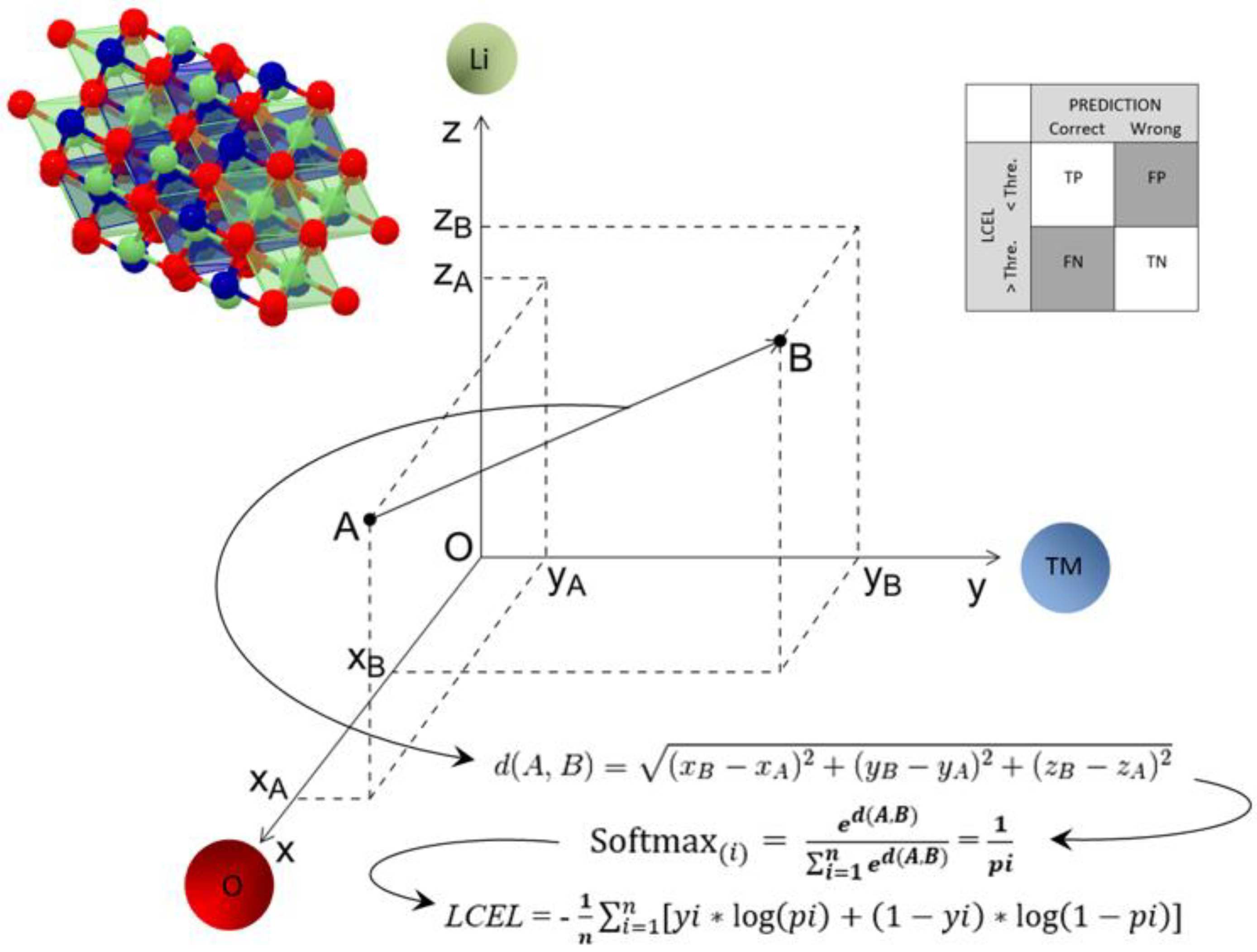
2.3. Distance Metric

Another key factor in ML algorithm is the distance metric. Among other, Euclidean distance is a widely used distance metric. It works on the principle of the Pythagoras theorem and signifies the shortest distance between two points. Mathematically, for an n-dimensional space and (pi, qi) as data points, the Euclidean distance metric is calculated using the following:

$$\mathit{d}={\left({\sum }_{\mathit{i}=1}^{\mathit{n}}{({\mathit{p}}_{\mathit{i}}-{\mathit{q}}_{\mathit{i}})}^2\right)}^{1/2}$$

(1)

In this work, the Euclidean distance was used as a metric to measure the similarity between the training compound and the one under testing. This has been made possible by the fact that the observations to be compared (chemical element and its stoichiometric coefficient) are continuous and have comparable numerical variables. In the formula, qi and pi are the stoichiometric coefficients of the ith element which constitutes the elementary cell formula of the compound to be analysed and of the training one, respectively.

2.4. Classification Model

The KNN method was used to classify the data point. KNN uses proximity to make classifications or predictions about the clustering of a single data point. Put simply, it captures information of all training cases and classifies new cases based on a similarity. Predictions are made for a new instance (x) by searching through the entire training set for the K most similar cases (neighbours) and summarizing the output variable for those K cases.

2.5. Space Group Prediction

The compound under test was compared with all those present in the training dataset and the proximity between the cell formulas was calculated. The first six compounds closest to the compound to be tested were then extrapolated. The Softmax function was used to normalize the outputs, converting them from weighted-sum values into probabilities that add up to one. Each value in the Softmax function output was interpreted as the membership probability for each space group. The compound under test was assigned the space group of the training compound that appeared with the highest percentage. At the end, for each of the n compounds forming the dataset, it is possible to have a prediction of the crystalline group to which it belongs.

2.6. Evaluation Metrics

Accuracy, precision, sensitivity, selectivity, F1 score, and false positive ratio (FPR) were used to evaluate the goodness of achieving results. The mathematical definition of these expressions can be found in Section 6 “Evaluation metrics” present within the Supplementary Materials.

The logarithmic cross-entropy loss (LCEL) was used to evaluate the goodness of the prediction. Cross-entropy is a measure of the difference between two probability distributions for a given random variable or set of events. Cross-entropy is widely used as a loss function when optimizing classification models. The closer the LCEL approaches to zero, the more reliable the prediction. For LCEL values equal to zero, the model is perfect. As the value of the LCEL increases, we have a decrease in the predictive efficacy of the model: for LCEL values lower than 0.3, we still have large margins of success in the prediction; however, for higher values, the model starts to falter.

A confusion matrix was used to determine the performance of the classification models. To predict a true/false label, a threshold value must be applied, and the threshold value affects the distributions of true/false labels. To correctly identify the threshold value, this was correlated to the LCEL value. If the value of the LCEL was less than the threshold value and the prediction was correct, the result was treated as a true positive. If the result had been wrong, it would have been a false positive. If the value of the LCEL was greater than the threshold value and the prediction was correct, the result was treated as a false negative. If the result had been wrong, it would have been a true negative. Figure 1 shows the workflow of the entire process.

3. Results

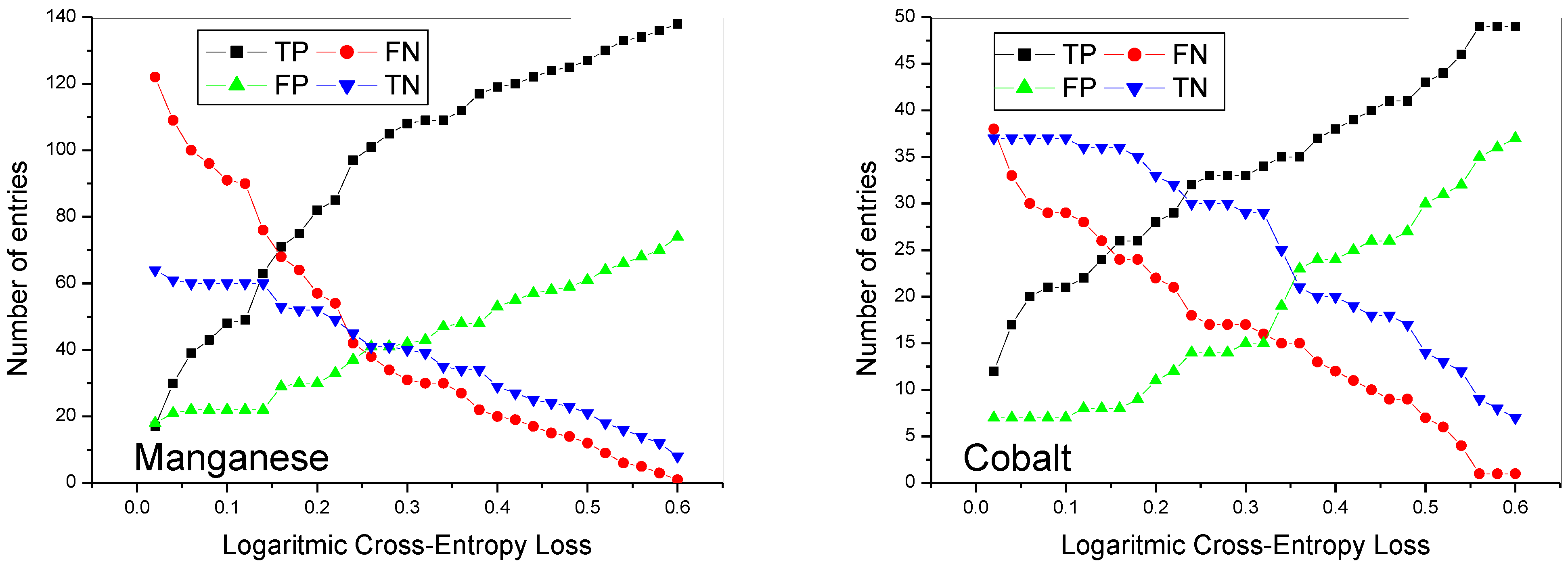
Figure 2 shows the number of true positives (TP), false negatives (FN), false positives (FP), and true negatives (TN) calculated for manganese and cobalt lithiated oxides as a function of the value of the LCEL. Although the graphs are different from each other, the trend of the curves is almost similar. For low threshold values there is a high number of false negatives. In fact, the model, although having correctly identified the crystalline group of the compound under test, fails to satisfy the requirement of a low LCEL value. Therefore, the forecast result, although correct, is considered wrong, increasing the number of false negatives. The number of true negatives is also high, while the number of true positives is low. Although cross-entropy is the theoretically preferred function for multi-label categorization [25], for low threshold values it happens that, being the class very unbalanced, the LCEL function suffers from the classic problem of unbalanced classes as it manages to predict many more true negatives than true positive [25]. This result is linked to the fact that the number of crystalline groups is very high (there are 230 different space groups in all); therefore, it is statistically easier for the compound under testing to be classified as true negative rather than true positive. False positives are very low as the model would have little chance of randomly identifying the correct crystalline group among the 230 available space groups. As it is logical to expect, as the value of the LCEL increases, there is an increase in both true and false positives and a decrease in true and false negatives. True positives are always greater than false positives. For both oxides, as the value of the LCEL increases, true positives increase at a higher rate than false positives. When the LCEL value reaches approximately 0.25, false positives begin to grow at a rate comparable to that of true positives. As far as manganese is concerned, for low values of the LCEL the false negatives are higher than the true negatives; however, for values higher than 0.25, there is a trend reversal. Subsequently, true and false negatives tend to decrease at the same rate.

In the case of cobalt, for low values of the LCEL, the false negatives are equal to the true negatives; however, as the LCEL increases, the true negatives remain constant while the false negatives decrease rapidly. Again, for LCEL values greater than 0.30, true and false negatives tend to decrease at the same rate. For this type of application, it is important, in addition to having a high number of true positives, to reduce the false positives, i.e., to avoid identifying compounds which apparently appear to belong to a determinate crystalline group and instead belong to another one. 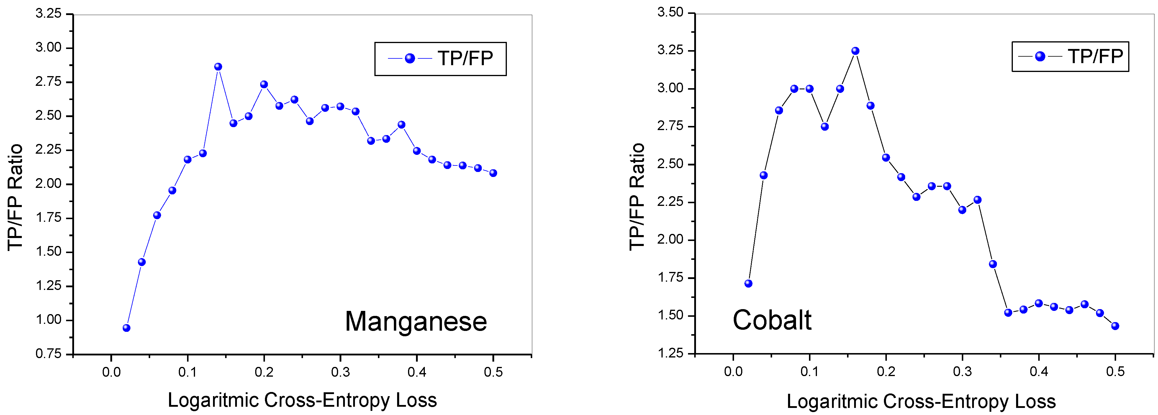Figure 3 shows the ratio between the number of true positives (TP) and that of false positives (FP) as a function of the LCEL value.

For both oxides, as the LCEL increases, there is a rapid increase in the ratio between true and false positives, which reaches values below three for manganese and above three for cobalt. However, with the increase in the LCEL value, while this ratio tends to remain constant for manganese at values higher than two, for cobalt it first drops to two and then, for LCEL values higher than 0.32, it undergoes a further decrease.

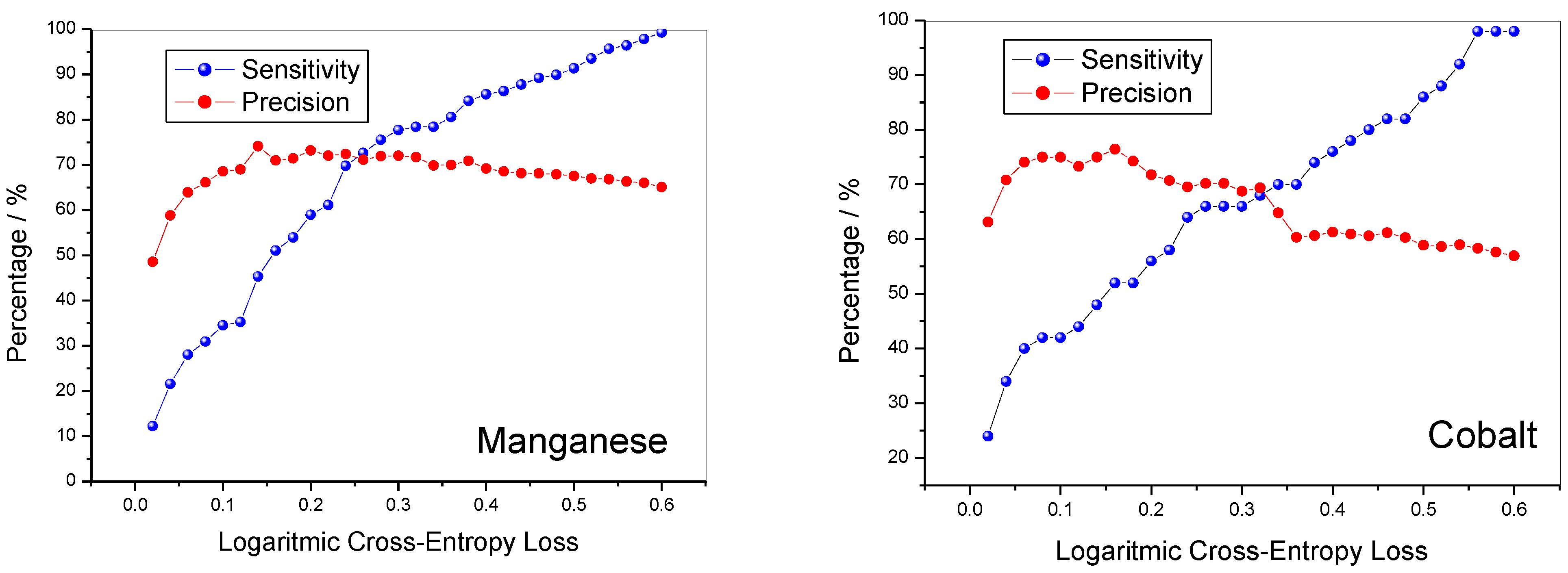
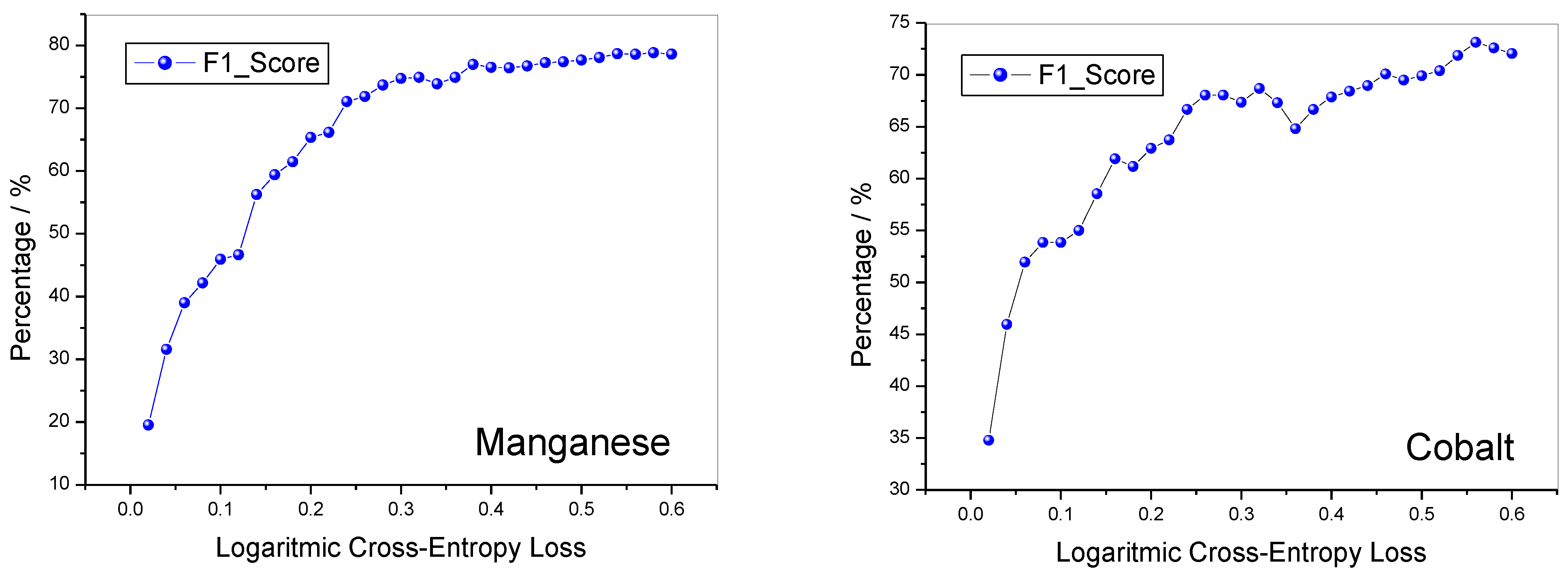
Sensitivity and precision as a function of LCEL are shown in Figure 4. Sensitivity is low for low LCEL values and tends to increase with increasing LCEL value. Precision however, after an initial increase, tends to decrease slightly as the LCEL value increases. For LCEL values between 0.2 and 0.3, precision values are placed in a range between 0.6 and 0.8, respectively. The two parameters are summarized in the value of the F1_Score whose value as a function of the LCEL are shown in Figure 5. Although the starting values of the F1 Score for manganese and cobalt lithiated oxides are different from each other, they tend to quickly increase with the increase in the LCEL value in both cases.

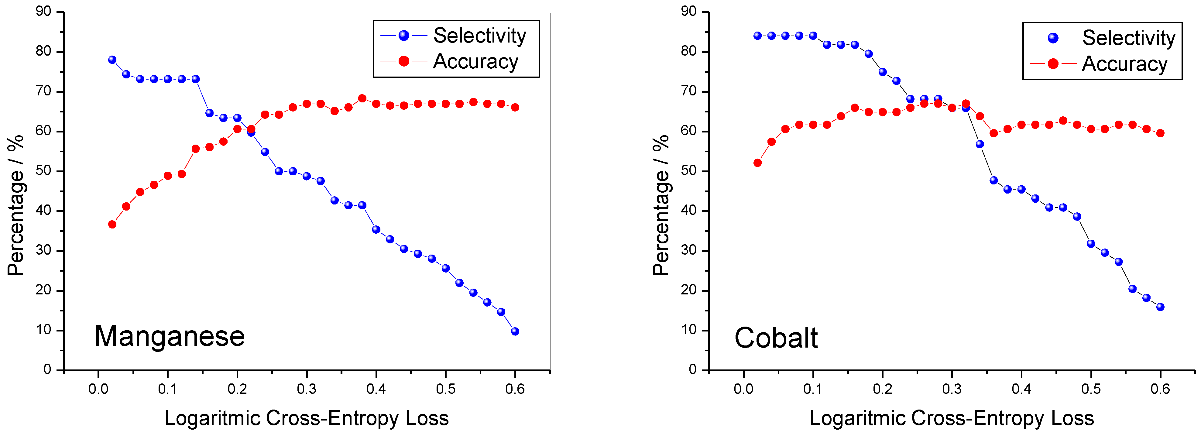
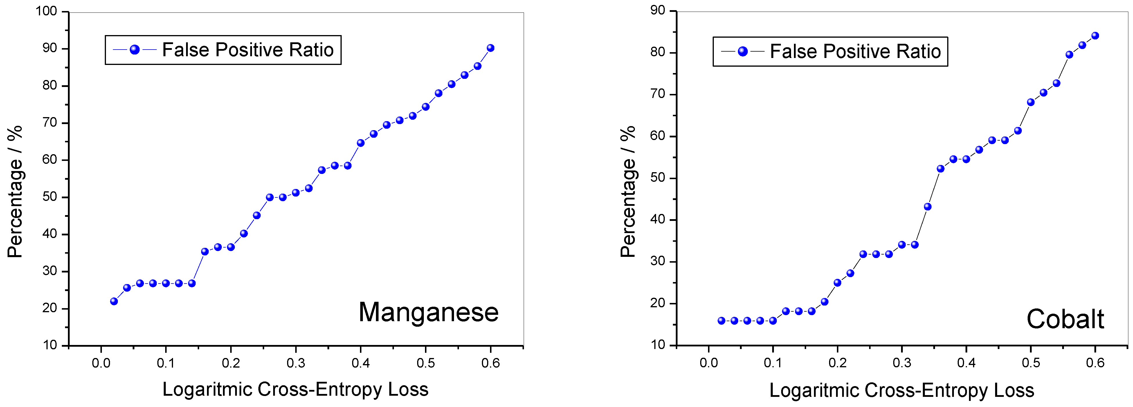
When the LCEL has reached a threshold value of 0.25, for both materials the value of the F1_Score reaches a value of 0.7 and does not change much for further increases in the LCEL. The selectivity and accuracy of the method are shown in Figure 6. For the lithiated manganese oxides, the selectivity value is slightly lower than 0.8, while for cobalt, it is slightly higher than this value and for both it remains almost constant until the LCEL value reaches 0.25. For further increases in LCEL, there is a steady decline in selectivity. The accuracy is slightly higher when the method is applied to cobalt oxides than to manganese ones; however, for LCEL values higher than 0.2, for both oxides the accuracy value is higher than 0.6. Finally, the FPR is reported in Figure 7. This value is more favourable for cobalt oxides than for manganese ones, but in any case, for small values of the LCEL, it is very low for both. For LCEL values lower than 0.14, the FPR value is lower than 0.26 for both oxides. As the LCEL increases, the FPR value is constant for both manganese and cobalt oxides.

4. Discussion

The choice of an appropriate threshold value of the LCEL is crucial to maximize the results obtained using the model. A threshold value of 0.3 brings several advantages. First, that of decreasing the number of false negatives in favour of true positives and this increases the probability to predict the crystalline structure of an unknown compound. At the same time, the risk of assigning to the test compound a crystalline structure that does not correspond to the truth increases. For this reason, assigning a lower threshold value considerably decreases this possibility but could exclude many true structures by marking them as false or true negative. In fact, this risk is very high for LCEL cut-off values below 0.20. From the obtained result, it is possible to state that a threshold of 0.25 could represent a good trade off to reduce the number of false positives maintaining good selectivity and high precision. Since some cobalt or manganese space groups may not be contained in the training dataset, the program is unable to predict these groups. A better approximation could be obtained by considering only the crystalline classes contained in the iron dataset. This model could be further implemented by generating a learning matrix that contains all three lithiated oxides of manganese, cobalt, and iron and using this matrix to predict the crystalline group of compounds not yet synthesized. Since only some crystalline compounds are capable of intercalating lithium ions, such as stratified materials or those with a spinel structure, the exact prediction of the crystalline group would allow for the directing of the synthesis exclusively towards those compounds which have a structure potentially suitable for interacting reversibly with lithium ions.