Interpretable Machine Learning Analysis of Stress Concentration in Magnesium: An Insight beyond the Black Box of Predictive Modeling

Abstract

In the present work, machine learning (ML) was employed to build a model, and through it, the microstructural features (parameters) affecting the stress concentration (SC) during plastic deformation of magnesium (Mg)-based materials are determined. As a descriptor for the SC, the kernel average misorientation (KAM) was used, and starting from the microstructural features of pure Mg and AZ31 Mg alloy, as recorded using electron backscattered diffraction (EBSD), the ML model was trained and constructed using various types of ML algorithms, including Logistic Regression (LR), Decision Trees (DT), Random Forest (RF), Naive Bayes Classifier (NBC), K-Nearest Neighbor (KNN), Multilayer Perceptron (MLP), and Extremely Randomized Trees (ERT). The results show that the accuracy of the ERT-based model was higher compared to other models, and accordingly, the nine most-important features in the ERT-based model, those with a Gini impurity higher than 0.025, were extracted. The feature importance showed that the grain size is the most effective microstructural parameter for controlling the SC in Mg-based materials, and according to the relative Accumulated Local Effects (ALE) plot, calculated to show the relationship between KAM and grain size, it was found that SC occurs with a lower probability in the fine range of grain size. All findings from the ML-based model built in the present work were experimentally confirmed through EBSD observations.

1. Introduction

Magnesium (Mg) and its alloys are among the most promising materials for several fields, including structural and medical applications [1]. This is due to its natural abundance (2.5%) and lightweight nature (33% and 75% lighter than aluminum and steel, respectively) [2]. In addition, Mg-based alloys exhibit both biocompatibility [3] and suitable mechanical properties [1] to be employed as implants in medical applications [4]. The mechanical properties, including strength, ductility, and toughness, of Mg alloys are mainly associated with their microstructural parameters, such as grain size and morphology, grain boundaries, and texture, which, in turn, evolve after the processing of these materials. Nowadays, there is huge interest in Mg-related research due to the high potentiality of these materials in various fields. Most of the work on Mg-based materials are focused on the improvement of mechanical performance. In this regard, ductility is one of those properties, which is in great need of improvement. To achieve that, various techniques, processes, and procedures have been used to control the microstructure of the targeted material, and thus to improve the ductility [1]. It is well known that the task of improving the ductility in Mg-based materials can be done successfully by a concrete understanding of the processing–microstructure–property relationships. Indeed, a huge number of studies have been conducted to solve the ductile issue in Mg-based materials using various strategies, and those are mostly experimental works [5,6,7], with some present works done based on computational methods (DFT [8] and MD [9]). Up to now, very few studies have discussed the application of data-based methods (machine learning (ML)) to figure out the relation between the structure and ductility of Mg materials. Very recently, these methods have received great interest by researchers in the various fields of medicine, science, and engineering. For example, in materials science and engineering, ML was used successfully to accelerate the discovery of new materials with high performance [10,11,12,13,14,15]. In this work, the built ML model intends to give an insight into the stress concentration and ductility relationship of Mg and AZ31 Mg alloy; specifically, the kernel average misorientation (KAM) is the chosen indicator of ductility that will be utilized and investigated. Generally, the KAM values reflect the residual stress level and dislocation density in the microstructure. Gui et al. [16] reports the KAM value evolution at specific levels in the tensile curve of Mg-4Y-3Nd-2Sm-0.5Zr alloy. Some conclusions can be withdrawn regarding the overall average KAM values: firstly, the average KAM value evolves incrementally with increased strain, as can be seen from the work done by Gui et al.; secondly, the distribution of KAM values in the sample highly relates to the residual stress concentration and dislocation density distribution, where the average KAM value increases as the strain increases up to the point where energy dissipation through cracks is initiated [16].

Up to here, the present work was designed to build an ML model through which structure–ductility relationship can be interpreted. For this purpose, experimentally collected data from two materials (pure Mg and AZ31 Mg alloy) were used in a learning process to build the model. This model, accordingly, relates the ductility (the output) and microstructural parameters, hereafter called features by known convention, including grain size, morphology, misorientation, and orientation.

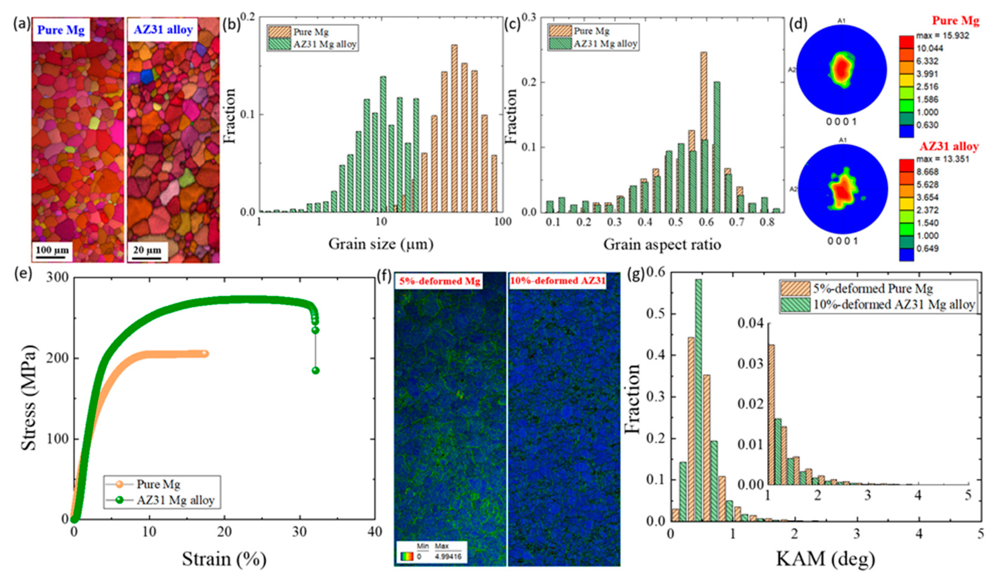
2. Materials and Experiments

Pure Mg in the form of hot-rolled plates used in the present work were supplied by Goodfellow Cambridge Limited (Huntingdon, UK). Rolled plates of AZ31 Mg alloy provided by POSCO (Pohang-si, Korea) was also used in the present work; in total 3 specimens were used for each material (pure Mg and AZ31 Mg alloy). The microstructural features of the as-received materials were characterized using electron backscattered diffraction (EBSD) in a scanning electron microscope (SEM). For electron back backscatter diffraction (EBSD), samples were prepared using a cross-sectional polisher (IM4000, Hitachi, Tokyo, Japan) and were observed by SEM (SU-5000, Hitachi, Chiyoda City, Tokyo) equipped with the EBSD analysis system (Velocity^TM Super, EDAX, Pleasanton, CA, USA). For detailed crystallographic orientation analysis, TSL, OIM version v8.6 (EDAX, Pleasanton, CA, USA) was used. For the EBSD-SEM observations, samples cut from a rolling direction–transverse direction (RD-TD) were prepared using mechanical grinding followed by cross-sectional polishing; the rolling-direction here was parallel to the tensile axis. Room-temperature tensile tests were conducted on a dog-bone-shaped sample cut from the two materials at a strain rate of 10⁻³ s⁻¹. Samples from the two materials were strained for 5 and 10%, respectively, and the microstructure evolution after the straining was observed using SEM-EBSD.

3. Learning Procedure

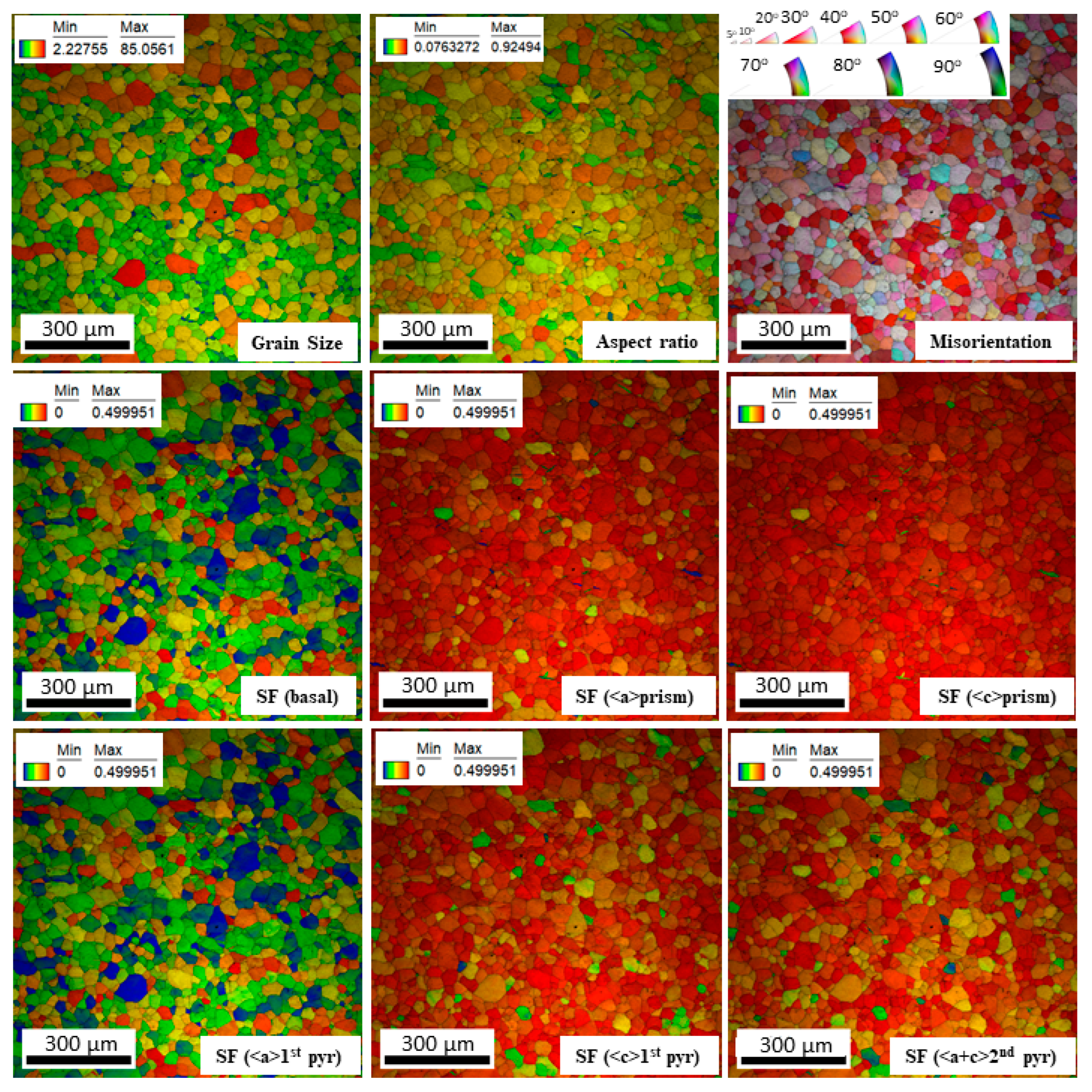
3.1. Microstructural Features

Before discussing the data to be used in the learning process employed in the present work, the microstructure, texture, and tensile properties of the pure Mg and AZ31 Mg alloy used in the present work were introduced and compared. Figure 1 summarizes the structure and properties of the pure Mg and AZ31 Mg alloy. In terms of grain structure, both materials exhibit an equiaxed grain morphology (Figure 1a), but with different sizes, where the grain size distribution in Figure 1b shows an average size of ~30 and ~10 µm in the pure Mg and AZ31 Mg alloy, respectively. The grain aspect ratios, in turn, were somehow similar in the two materials, where average ratios of 0.6 and 0.65 were recorded for pure Mg and AZ31 Mg alloy, respectively (Figure 1c). The texture of the two materials presented by the (0001) pole figures in Figure 1d show that both materials (pure Mg and AZ31 alloy) exhibit a strong basal texture, and that was stronger in the pure Mg as compared to that of AZ31 Mg alloy, as shown by the maximum intensities (15 vs. 13, Figure 1d). The room-temperature tensile curves presented in Figure 1e show the expected behaviors, in which the pure Mg exhibited less ductility as compared to that of AZ31 Mg alloy, indicating the more brittle nature of this pure Mg sample. The main and the well-known reason that explains the brittleness in pure Mg is the lack of slip systems that can be operated at room temperature [17]. This, in turn, is related to the gap between the critical resolved shear stresses (CRSS) of the various slip systems. For example, at room temperature, the CRSS of the pyramidal slip system is 100 times bigger than that of the basal slip system, and due to this nature, only the basal slip system containing 3 distinct slip systems, where 2 of them are independent systems, will be available at room temperature. Considering the 5 required independent slip systems, as determined by the von Mises criterion [17,18], the 2 independent basal systems are not enough to achieve a uniform deformation in the material, leading to a non-uniform deformation, stress concentration, and, finally, to early fracture in this material. Generally, the stress concentration caused due to the non-uniform deformation is followed using the kernel average misorientation (KAM) measurements, which are easily reached through EBSD observations. The KAM values represent the concentration of geometrical necessary dislocations activated during the plastic deformation [19]. This, in fact, can be an implicit indicator of ductility in a material, as discussed earlier. In the present experiments, pure Mg and AZ31 Mg alloy samples were strained into 5% and 10%, respectively, and the EBSD measurements were conducted to determine the microstructural parameters of the deformed samples. Those strains were basically chosen according to the full tensile behaviors of the samples (Figure 1e), where those are in the range of approximately 30% from the total elongation of the counterpart sample. The KAM measurements (maps and profiles) of the 5%-strained Mg and 10%-strained AZ31 alloy in Figure 1f,g show that, even though the amount of strain applied on the pure Mg sample was less than that applied on the AZ31 Mg alloy sample, this sample exhibited a higher KAM, suggesting that the stress concentration occurred more frequently in the pure Mg sample, which resulted in its lower ductility as compared to the AZ31 Mg alloy. Up to here and in order to understand how structural parameters influence the stress concentration in the Mg samples investigated in the present work, those parameters, including grain size, morphology (aspect ratio), misorientation, and orientation, were collected based on the EBSD observations, as shown by the maps presented in Figure 2. The data of 4694 grains from the two materials (pure Mg and AZ31 alloy) was collected. In addition to those parameters, the applied strain (5 and 10% in pure Mg and AZ31 alloy, respectively) and the composition of these materials were also considered in the basic feature space used in the learning process. In terms of the grain orientation, the Schmid factor (SF) of various slip systems was employed as a feature, and here, basal slip, <a> prismatic slip, <c> prismatic slip, 1st order <a> pyramidal slip, 1st order <c> pyramidal slip, 2nd order <a + c> pyramidal slip, were considered (Figure 2). To show the distribution of the collected features, their histograms are presented in Figure 3. Table S1 shows the features used in this work in more detail.

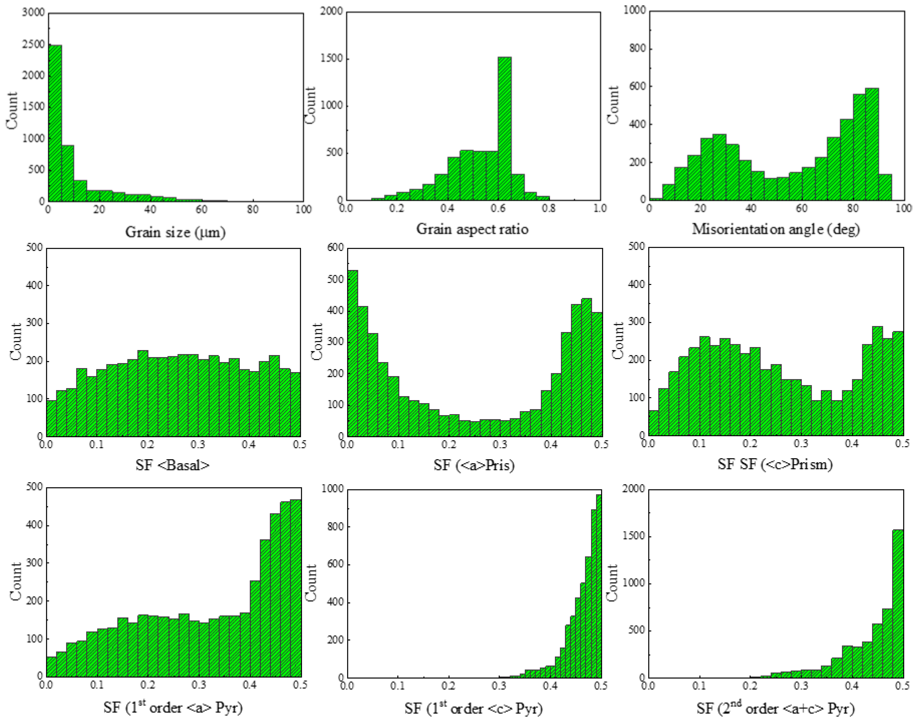
3.2. Features Engineering

Based on the established features mentioned before—let us call them basic or elemental features for the rest of this article—we opted to increase this elemental feature space by including different mathematical transformations such as sine, cosine, exponential, mean, standard deviation, and summation, to name a few. Table S2 shows a full list of the features that were generated alongside their base features that were built upon. This expansion of the feature space serves two main purposes that need to be clarified: The first is that mathematical transformations of already-set features will lead to a better performance of the predictive model overall [20]. This is due to the fact that a normal distribution in ML is the most desirable distribution that will increase the predictive capability of the model significantly because a normal distribution, simply put, makes the math easier. Most ML/DL algorithms and architectures in their innerworkings assume a normal distribution; i.e., they are derived from a normal distribution assumption. The data distribution in this work is hardly ever normal in their nature, as shown in Figure 3; the grain aspect ratio, for example, is as normal as it gets in the elemental feature space followed by SF <Basal>. Other elemental features, such as the grain size, for example, follows a Poisson distribution. The second purpose for expanding the feature space to include different mathematical transformations is simply to enhance the interpretability of the predictive model. This interpretability is mainly associated with not only understanding which feature contributes the most to the model, which can be interpreted by experimental insight, but also at which mathematical format (log, sine, cosine, etc.) it is more likely to be at, giving an analytical edge to the constructed model that can be used in a further step to construct a compact and comprehensive equation [21]. Most of the transformations that are used in this work are non-linear; therefore, it reduces the possibility of our model being too complex by incorporating many linearly correlated features that serve no purpose but to overcomplicate our model and render it overfitted in many cases. All in all, this feature-engineering process has resulted in 53 features, as presented in Table S2.

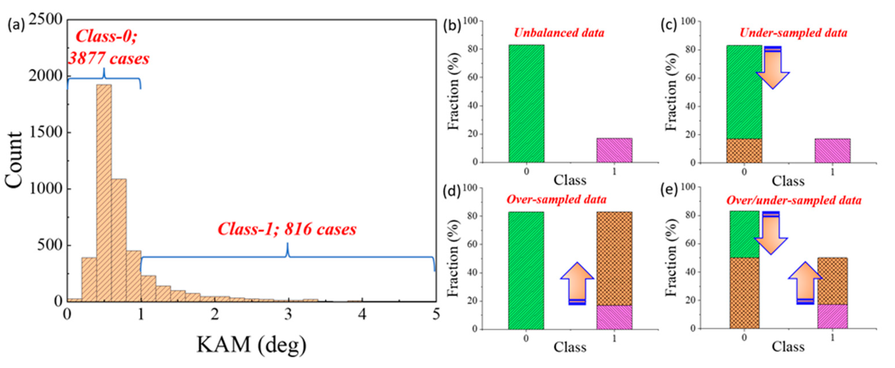
3.3. Initial Dataset and Data Analysis

In the initial stages, the data that were collected for the 5%-strained pure Mg and 10%-strained AZ31 alloy combined showed a predicted imbalance in the range of KAM, with an average of 0.78°, a variance of 0.34, and a standard deviation of 0.12. The skewness of the collected data was calculated and is 3.31 with a kurtosis of 13.8. This suggests that the distribution of the collected data is highly narrow and positively skewed, as shown in Figure 4a. This distribution is a sign of an imbalanced dataset that is to be balanced before classification goes underway. One way to balance these data is to choose a suitable classification threshold that virtually separates the data into equal chunks of two classes. This is impractical and overexaggerated when viewed from a material science perspective. In our collected data and based on the previous simplified statistical analysis, a statistical classification threshold for the KAM would suggest that anything less than the average (0.78°) is a suitable starting point for this binary partition that would, more or less, ensure that the imbalance is alleviated. Yet, this classification threshold is a problem-specific quantity, and in this problem, what constitutes the boundary between high and low KAM classes, is highly related to the material and specific distribution of the high KAM values. Thus, to remedy this problem, we are going to suggest a rather more compact and realistic threshold, which is an average KAM (0.78°) and the addition of a one standard deviation step and rounding it up to a KAM value of 1°; this value assures that the KAM values over 1° give a higher possibility for stress to be concentrated within those grains that are in the remaining 15~20%, which, as Figure 4a shows, is 816 cases. From a material science perspective, this threshold could be based on a study by Wright et al., where a microstructure can be regarded as a highly deformed structure if its average KAM value is higher than 1° [22], which could rationalize our choice of KAM threshold that was solely based on statistical analysis. The other way of balancing the data in this case, as will be expanded upon later in this work, is by utilizing the different resampling techniques for the collected data. To understand this issue deeper, Figure 4b–e shows a simple overview of those techniques in action. For a specific imbalanced dataset, as is presented in Figure 4b, one can observe how the class imbalance is obvious. Class “0”, which in this case represents the KAM values of less than 1°, practically represents a more than 80% fraction from the dataset that was used, leaving the remaining 20% for the other class, “1”, which represents KAM values that are more than 1°. This statistical imbalance can be mitigated by either under-sampling the majority class (“0” in this case), which is represented in Figure 4c, over-sampling the minority class (Figure 4d), or a hybrid approach, where a compromise is reached between the two techniques, as shown in Figure 4e; other techniques in dealing with imbalanced datasets are active learning [23], cost-sensitive learning [24], and kernel-based methods [25]. The resampling techniques that were used in this work, i.e., over-sampling and under-sampling, both have their pros and cons, and the following discussion will expand upon a few of both [26]. The first is that an imbalanced dataset is detrimental to the operation of the model and its ability to learn both classes equally, which leads to, in many cases, a misleading accuracy assessment if the practitioner is not aware. The second benefit of one of those techniques, namely, over-sampling, is that the data-balancing technique comes at no cost of the original data, meaning that the additional data generated or “synthesized” are used to enhance the predictive and exploratory capability of the model with no information loss. Of course, in the ML research field, there are no free lunches, and certainly resampling techniques are not exempt from that statement. Over-sampling, for instance, synthesizes new data that are generated based on a proximity algorithm that establishes new “guesstimated” points, as will be shown in the next sections, that are as close as possible to the original minority class in the feature hyperspace [26]. This procedure is an augmentative one, and with this comes authenticity questions that are no doubt quite philosophically challenging. However, the methodology works [27] and this work will show how it can be utilized in the study of stress concertation using KAM measurements obtained from Mg and AZ31 alloy. Under-sampling, on the other hand, reduces the amount of data that are used in the training process by restricting or deleting the majority classes in favor of balancing out the minority. This process introduces information loss that will reduce the predictive and exploratory power of the model. As a concluding statement, the resampling techniques mentioned above are not to blame for arising those concerns about data integrity; this issue stems from the data imbalance problem itself, which over-sampling and under-sampling try to solve and are reported to be quite successful at that [26]. After identifying the issues that we are to face after the short Exploratory Data Analysis (EDA) that was done earlier. We opted to use over-sampling and a hybrid mixture of both to deal with the imbalanced data. Over-sampling techniques used in this work are random over-sampling and the Adaptive Synthetic approach for imbalanced data (ADASYN). For the hybrid approach, a SMOTE-Tomek algorithm was used. Random over-sampling and under-sampling are virtually identical, but where in random over-sampling the minority class dataset is duplicated with replacement to enlarge this category to a point where it has a similar size as the majority class. This technique is very prone to overfitting, which is considered by most ML practitioners to be very unreliable in the context of predictive modeling. The second technique is ADASYN, which is an adaptive method that was first proposed by He et al. [28], and utilizes the idea of proximity between points of the same class to generate new data points with similar features to original minority classes. This is similar to the workings of the Synthetic Minority Over-sampling Technique (SMOTE) [29], which utilizes the Euclidean distance between each minority points for data syntheses but each point in the minority class is assigned a density distribution to create new points according to its nearest neighbors and their classes in a scattering fashion rather than strictly linear as in SMOTE. A hybrid approach called SMOTE-Tomek includes operating both methods of over-sampling and under-sampling in tandem, where minority class data are increased and majority class data are decreased simultaneously; using this technique affirms that the data is minimally augmented while a considerable amount of information remains, thus decreasing both information loss and gross overfitting (a discussion about the mathematical formulation of those algorithms is given in the Appendix A).

3.4. Training and Testing

In the training process, we have opted to use a myriad of different classification algorithms that allow us to explore different classification approaches with different innerworkings, such as Logistic Regression (LR) [30], Naive Bayes Classifier (NBC) [31], K-Nearest Neighbor (KNN) [32], Multilayer Perceptron (MLP) classifier [33], Decision Trees (DT) [34], Random Forest (RF) [35], and Extremely Randomized Trees (ERT) [36]. These algorithms were primarily used to construct an optimum classifier that is capable of distinguishing between low and high stress concentration in individual grains based on collected data from experimental EBSD analysis. Before delving into the results of the training and establishing the interpretability analysis, it is imperative to discuss the classification metrics that will be used to assess the model. It is conventional to use a confusion matrix as a basis for accuracy measurements in a specific classification procedure [37]. A confusion matrix consists of positive predictions (in this case, KAM > 1°) that are correctly predicted, called true positives (TP), and the countering incorrect ones, called false positives (FP). The same applies for negative predictions (KAM < 1°) that are correctly and incorrectly predicted, as mentioned before called true negatives (TN) and false negatives (FN), respectively. A robust model tends to decrease FNs and FPs as much as possible, but there is an inherent tradeoff here between a model that can correctly predict TP and TN. To assess the accuracy of the models on hand, accuracy and F1-score were used. Accuracy is a metric that is defined by the following equation [37]:

$$\mathrm{Accuracy}=\frac{\mathrm{TP}+\mathrm{TN}}{\mathrm{TP}+\mathrm{TN}+\mathrm{FP}+\mathrm{FN}}$$

(1)

Although this metric seems fairly reliable at first, it is not. In this work, it is obvious that this metric will be high regardless of the actual performance. This is by in large due to the fact that our original data are imbalanced by default, which means that even if the classifying algorithm is based on choosing a negative prediction every time, it will show a high accuracy (80%) by virtue of having an 80/20 proportion between the negative and positive classes. Therefore, due to the previous fact, ML practitioners have introduced two additional flagship accuracy measures that give more insight into how an ML model is behaving. These are recall and precision, and in mathematical terms they are defined by the following equations [37]:

$$\mathrm{Precision}=\frac{\mathrm{TP}}{\mathrm{TP}+ \mathrm{FP}}$$

(2)

$$\mathrm{Recall}=\frac{\mathrm{TP}}{\mathrm{TP}+\mathrm{FN}}$$

(3)

Precision, in simple terms, represents how many of the predicted positives are actually true according to our initial dataset; this is to assess if the model is capable of capturing true negatives in its prediction. Recall, however, represents how many of our positive values were correctly classified; therefore, it is a measure of how good our model is in predicting true positives. Both emphasize different quantities of prediction, and because in our work we are to require a balanced importance of high and low KAM regions without discrimination, the F1-score measure was used; this measure is defined as the harmonic mean of the recall and precision [37]:

$$\mathrm{F}1 \mathrm{score}=2 \frac{\mathrm{Precision}\times \mathrm{Recall}}{\mathrm{Precision}+\mathrm{Recall}}$$

(4)

This score gives a clear image of the model’s performance without prioritizing a specific class over another (high KAM or low KAM); thus, it can be used to compare between different models. The 10 k-fold cross-validated accuracy and F1-scores of the used models are provided in Figure 5. Specifically, Figure 5a represents unbalanced data; Figure 5b random over-sampling; Figure 5c over-sampling with ADASYN; and Figure 5d the hybrid approach of over/under-sampling using SMOTE-Tomek. It is clearly shown that the imbalance in the data affected the results and using the resampling techniques helped in overcoming this issue. The highest accuracy and F1-score between these models were recorded for the ERT algorithm, with a 0.89 score for the hybrid over/under-sampling technique; therefore, this model can be used for further analysis.

4. Results and Discussions

After training and testing the various ML-based models using the different data balancing techniques, the final model (ERT-based model) with the highest score in this grid (resampling technique and ML algorithm) was chosen for further inspections. Here, interpretability is the main objective of ML, and will be used for that purpose through feature important analysis that will be laid out in the rest of the work. The top 9 important features in this model (ERT), those with a higher decrease in Gini impurity [38] than others, were extracted and are shown in Figure 6a. Here, the logarithmic transformation of the grain size is the most important feature, with an impurity of 0.083. Interestingly, grain size has contributed the most of these features—7 features out of the 9—confirming the significant effect of grain size on the plasticity and SC of Mg-based materials. Of course, this observation can be done experimentally by examining the relationship and coming to the same conclusion based on expertise; yet, here it is important to know which mathematical transformation of grain size gives a stronger correlation, and thus it can help immensely in further modeling and for mathematical equation formulation of the stress concentration based on KAM measurements, increasing the accuracy and interpretation of such models. To show how a feature is significant, a global model-agnostic interpretability measure—the min–max normalized relative Accumulated Local Effects (ALE) [39] (more information about the normalization process is given in the Supplementary Materials) plots—are presented for some targeted features; those plots describe the 1st-order effects of the features and are shown in Figure 6b, and this metric reflects the dependency of the output (KAM) on the feature, where higher values of relative ALE indicate that the stress concentration (KAM > 1°) is more likely to occur as compared to lower values (a short discussion about ALE is given in Appendix A). A quick note would be necessary here regarding the choice of the interpretability metric between the Partial Dependence Plots (PDP) or ALE, as the rationale is that most of the features used in this work are indeed interrelated to one another making the partial dependence plots useless in our case [40]. Out of the 9 features presented in Figure 6a, 4 features were selected to show their counterpart relative ALE plots, and those are log (GS), exp[H(GS*AR)], SF (<c> prism), and SF (<a> prism) (Figure 6b). The results presented in Figure 6b reveal a complicated trend in the relative ALE probability as a function of the selected features, reflecting the complex nature of structure–property relationships in metals. For example, in the case of log GS (Figure 6b), the relative ALE value was found to be higher in the range of ultrafine-grained structure (GS < 1 µm), and it decreased by increasing the grain size to get a minimum value between 1.3 and 3.5 µm followed by another increase in the ALE value in the range of 14 to 20 µm. A similar trend of decreasing and increasing was also noted for the exp[H(GS*AR)]. Differently, in the case of SF, for both <a> and <c> prismatic slips, the relative ALE was high at an SF of ~0.45.

Considering the finding of the ML model reached in the present work, the GS is an important parameter that highly influences the KAM formation during straining of Mg-based materials, especially in the range of finer-grained structures; however, one can question the interpretation of these results. The low (minimum) ALE values noted between 1.3 and 3.5 µm can be explained based on the occurrence of grain boundaries sliding as an additional softening mechanism, leading to a lower accumulation of dislocations, and accordingly, less stress concentrations. The occurrence of such a mechanism in this range of grain size was introduced by Zeng et al. [41], who reported the occurrence of grain boundaries sliding in the near-micron grains of pure Mg samples extruded at 80 °C, and that happened at the expense of the other in-grain mechanisms, including dislocation slip and twinning. This reduces the probability to build the in-grain stress needed for fracture. On the other hand, the higher relative ALE values of the grains with a size between ~14 and 20 µm can be attributed to the twinning ability in this range of grain size, where it is well-known that the twining activity increases with increasing the grain size [42,43]. Indeed, the evolution of twins were noted more frequently in the coarse grains (>10 µm). To confirm this point, two grains were chosen from the 5%-deformed pure Mg samples to be analyzed separately, and this is summarized in Figure 6c–g. As shown by Figure 6f, the two selected grains were twinned due to the plastic deformation, and the related twin boundaries (TBs) measured by point-to-point misorientation profiles across those twins (Figure 6f) indicated that those represent TBs of ~86° $〈11\overline{2}0〉$, which, in turn, are the characteristic of $\left\{10\overline{1}2\right\}$ extension twins. Figure 6g shows the evolution of a high KAM within and round these twins, which is in good agreement with the increase noted in the relative ALE plot of the log GS, in the range of ~14 to 20 µm, as presented in Figure 6b.

Back to the tensile behavior in Figure 1e, due to the grain boundaries strengthening effect, as reflected by the flow stress in Figure 1e, the lower stress recorded for the pure Mg can lead to increased activation of the basal slip systems due to their lower CRSS as compared to non-basal systems [44]. On the other hand, more non-basal dislocations can be generated within the fine grains of the AZ31 Mg alloy, and this is related to the higher flow stress of the AZ31 Mg alloy (Figure 1e). The lack of slip systems in the case of the coarse-grained structure of pure Mg, where the basal family with three independent systems is majorly available, resulted in the activation of other deformation modes to accommodate the plastic strain [45]. Here, a considerable number of twin boundaries (TBs) was detected in the 5%-deformed pure Mg sample, where those formed ~6% of the total high angle boundaries (HABs), as shown by the red line in Figure 6d. Even though twins contribute as a secondary deformation mode, which can contribute to accommodate the plastic strain, those twins can evolve some characteristics [45], which, in turn, induce the crack initiation and prorogation, finally leading to an earlier fracture.

To conclude the discussion of using ML for interpretability of physical systems and especially stress concentration in Mg and its alloys, it must be reminded that, for interpretability to be useful, one should assure that the design loop for the work conducted be sound and applicable to a reasonable extent. For this work, Figure 7 shows the design strategy that motivates the flow of this work.

First, the question that was needed to be answered is how can we get statistical insight into the stress concentration of Mg and its alloys; the answer is to find a suitable established descriptor, namely, a kernel average misorientation (KAM), that enables qualitative and special recognition of the stress concentration, which itself is hard to experimentally quantify and track as a function of microstructural features. Next, one must mine the data that is useful for this kind of analysis, and in this work, the experimental EBSD data of 5%-strained and 10%-strained Mg and AZ31 alloy, respectively, were obtained to construct a dataset. Then two of the most important questions must be asked: The first is the question regarding which method of machine learning is more useful for the job at hand given the category of the model that is to be constructed—an explanatory model that is interested in understanding the relations between features and outputs or a predictive model that is more oriented towards making an informed prediction, keeping in mind that interpretability and prediction are not mutually exclusive and can be used in tandem, but a more informed and uniform direction of ML modeling reduces redundant information and effort, to further explain whether regression, classification, or clustering is more useful and which of them has a better insightful direction for the project at hand. In this work, classification is certainly more important, as our target is not to predict KAM values of new instances and recognize stress concentration hotspots according to previous data, but to interpret the outcomes of the data in terms of the relationship between the input features and output response based on a binary classification process of the existing data at a specific threshold (KAM > or < 1°). The second important question to be asked is how to extract a useful feature space from the available parameters of measurement. The elemental features, shown in Figure 7, were organized so as to give the maximum amount of information about the material, such as the microstructural parameters, strain, and composition. Those elemental features can be further expanded using basic mathematical transformations to enhance the interpretability and utility of the feature space, as explained earlier. Then, ML, data balance (if the data are unbalanced), and interpretability algorithms and methods should be carefully chosen according to accuracy and interpretability measurements. For example, here, we used a hybrid over/under-sampling technique (SMOTE-Tomek) for balancing the data as well as an Extremely Randomized Trees Classifier for the classification process. This was followed by interpretability using feature importance and relative ALE plots, as shown in Figure 6. All in all, Figure 7 gives the necessary workflow that can be followed for an interpretable ML project; however, it is by no means a strict plan to be followed, but it can be used as the starting ground for more interpretable modeling, which is critically needed in the fields of material science and engineering.

5. Conclusions

This work was designed to construct an interpretable machine learning model that can be employed to give insight into the stress concentration in magnesium-based materials. This was done by training data containing the microstructural parameters obtained from pure magnesium and AZ31 alloy. The following points can be drawn from this study:

The ML model based on Extremely Randomized Trees (ERT) was successfully built with a high accuracy and an F1 score of ~0.89 for both.

The feature importance in the ERT-based model analyzed using the Gini impurity and the relative ALE plots showed that grain size is the most important factor to control the stress concentration, and that was significant in the logarithm-transformed form of the elemental feature of grain size.

The ML results reached in this study were in good agreement with the metallurgical aspects of magnesium and its alloy.

Lastly, this work is set to increase the applicability of ML techniques as interpretation methods rather than as conventional black box modeling in material science.

References

1. Chaudry, U.M.; Tekumalla, S.; Gupta, M.; Jun, T.-S.; Hamad, K. Designing highly ductile magnesium alloys: Current status and future challenges. Crit. Rev. Solid State Mater. Sci. 2021, 47, 194–281. [Google Scholar] [CrossRef]
2. Prasad, S.V.S.; Verma, K.; Mishra, R.K.; Kumar, V.; Singh, S. The role and significance of Magnesium in modern day research-A review. J. Magnes. Alloy. 2021, 10, 1–61. [Google Scholar] [CrossRef]
3. Chen, J.; Tan, L.; Yu, X.; Etim, I.P.; Ibrahim, M.; Yang, K. Mechanical properties of magnesium alloys for medical application: A review. J. Mech. Behav. Biomed. Mater. 2018, 87, 68–79. [Google Scholar] [CrossRef] [PubMed]
4. Chaudry, U.M.; Farooq, A.; Malik, A.; Nabeel, M.; Sufyan, M.; Tayyeb, A.; Asif, S.; Inam, A.; Elbalaawy, A.; Hafez, E.; et al. Biodegradable properties of AZ31-0.5Ca magnesium alloy. Mater. Technol. 2022, 1–12. [Google Scholar] [CrossRef]
5. Chaudry, U.M.; Hamad, K.; Ko, Y.G. Effect of calcium on the superplastic behavior of AZ31 magnesium alloy. Mater. Sci. Eng. A 2021, 815, 140874. [Google Scholar] [CrossRef]
6. Liu, B.-Y.; Zhang, Z.; Liu, F.; Yang, N.; Li, B.; Chen, P.; Wang, Y.; Peng, J.-H.; Li, J.; Ma, E.; et al. Rejuvenation of plasticity via deformation graining in magnesium. Nat. Commun. 2022, 13, 1060. [Google Scholar] [CrossRef]
7. Han, G.; Noh, Y.; Chaudry, U.M.; Park, S.H.; Hamad, K.; Jun, T.-S. {10–12} extension twinning activity and compression behavior of pure Mg and Mg-0.5Ca alloy at cryogenic temperature. Mater. Sci. Eng. A 2022, 831, 142189. [Google Scholar] [CrossRef]
8. Muzyk, M.; Pakiela, Z.; Kurzydlowski, K. Generalized stacking fault energy in magnesium alloys: Density functional theory calculations. Scr. Mater. 2012, 66, 219–222. [Google Scholar] [CrossRef]
9. Mahata, A.; Sikdar, K. Molecular dynamics simulation of nanometer scale mechanical properties of hexagonal MgLi alloy. J. Magnes. Alloy. 2016, 4, 36–43. [Google Scholar] [CrossRef]
10. Jaafreh, R.; Kang, Y.S.; Hamad, K. Lattice Thermal Conductivity: An Accelerated Discovery Guided by Machine Learning. ACS Appl. Mater. Interfaces 2021, 13, 57204–57213. [Google Scholar] [CrossRef]
11. Jaafreh, R.; Kang, Y.S.; Kim, J.-G.; Hamad, K. Machine learning guided discovery of super-hard high entropy ceramics. Mater. Lett. 2022, 306, 130899. [Google Scholar] [CrossRef]
12. Jaafreh, R.; Abuhmed, T.; Kim, J.-G.; Hamad, K. Crystal structure guided machine learning for the discovery and design of intrinsically hard materials. J. Mater. 2021, 8, 678–684. [Google Scholar] [CrossRef]
13. Zhang, Z.; Tehrani, A.M.; Oliynyk, A.O.; Day, B.; Brgoch, J. Finding the Next Superhard Material through Ensemble Learning. Adv. Mater. 2021, 33, e2005112. [Google Scholar] [CrossRef]
14. Ward, L.; Liu, R.; Krishna, A.; Hegde, V.I.; Agrawal, A.; Choudhary, A.; Wolverton, C. Including crystal structure attributes in machine learning models of formation energies via Voronoi tessellations. Phys. Rev. B 2017, 96, 24104. [Google Scholar] [CrossRef]
15. Tehrani, A.M.; Oliynyk, A.O.; Parry, M.; Rizvi, Z.; Couper, S.; Lin, F.; Miyagi, L.; Sparks, T.D.; Brgoch, J. Machine Learning Directed Search for Ultraincompressible, Superhard Materials. J. Am. Chem. Soc. 2018, 140, 9844–9853. [Google Scholar] [CrossRef] [PubMed]
16. Gui, Y.; Li, Q.; Xue, Y.; Ouyang, L. Twin-twin geometric structure effect on the twinning behavior of an Mg-4Y-3Nd-2Sm-0.5Zr alloy traced by quasi-in-situ EBSD. J. Magnes. Alloy. 2021. [Google Scholar] [CrossRef]
17. Chaudry, U.M.; Hamad, K.; Kim, J.-G. On the ductility of magnesium based materials: A mini review. J. Alloy. Compd. 2019, 792, 652–664. [Google Scholar] [CrossRef]
18. Dieter, G.E.; Bacon, D. Mechanical Metallurgy; McGraw-Hill: New York, NY, USA, 1988. [Google Scholar]
19. Seret, A.; Moussa, C.; Bernacki, M.; Signorelli, J.; Bozzolo, N. Estimation of geometrically necessary dislocation density from filtered EBSD data by a local linear adaptation of smoothing splines. J. Appl. Crystallogr. 2019, 52, 548–563. [Google Scholar] [CrossRef]
20. Zheng, A.; Casari, A. Feature Engineering for Machine Learning: Principles and Techniques for Data Scientists; O’Reilly Media, Inc.: Boston, MA, USA, 2018. [Google Scholar]
21. de Franca, F.O.; Aldeia, G.S.I. Interaction–Transformation Evolutionary Algorithm for Symbolic Regression. Evol. Comput. 2021, 29, 367–390. [Google Scholar] [CrossRef]
22. Wright, S.I.; Nowell, M.M.; Field, D.P. A Review of Strain Analysis Using Electron Backscatter Diffraction. Microsc. Microanal. 2011, 17, 316–329. [Google Scholar] [CrossRef]
23. Ertekin, S.; Huang, J.; Giles, C.L. Active learning for class imbalance problem. In Proceedings of the 30th Annual International ACM SIGIR Conference on Research and Development in Information Retrieval, Amsterdam, The Netherlands, 23–27 July 2007. [Google Scholar] [CrossRef]
24. Elkan, C. The foundations of cost-sensitive learning. In Proceedings of the International Joint Conference on Artificial Itelligence, Seattle, WA, USA, 4–10 August 2001; pp. 973–978. [Google Scholar]
25. Wu, G.; Chang, E. KBA: Kernel boundary alignment considering imbalanced data distribution. IEEE Trans. Knowl. Data Eng. 2005, 17, 786–795. [Google Scholar] [CrossRef]
26. Mohammed, R.; Rawashdeh, J.; Abdullah, M. Machine Learning with Oversampling and Undersampling Techniques: Overview Study and Experimental Results. In Proceedings of the 2020 11th International Conference on Information and Communication Systems (ICICS), Irbid, Jordan, 7–9 April 2020; pp. 243–248. [Google Scholar] [CrossRef]
27. Glazkova, A. A Comparison of Synthetic Oversampling Methods for Multi-class Text Classification. arXiv 2020, arXiv:2008.04636. [Google Scholar]
28. He, H.; Bai, Y.; Garcia, E.A.; Li, S. ADASYN: Adaptive synthetic sampling approach for imbalanced learning. In Proceedings of the IEEE International Joint Conference on Neural Networks, Hong Kong, China, 1–8 June 2008; pp. 1322–1328. [Google Scholar] [CrossRef]
29. Chawla, N.V.; Bowyer, K.W.; Hall, L.O.; Kegelmeyer, W.P. SMOTE: Synthetic Minority Over-sampling Technique. J. Artif. Intell. Res. 2002, 16, 321–357. [Google Scholar] [CrossRef]
30. Cramer, J. The Origins of Logisitic Regression. Tinbergen Institute Working Paper No. 2002-119/4, December 2002. Available online: https://papers.ssrn.com/sol3/papers.cfm?abstract_id=360300 (accessed on 10 August 2022).
31. Domingos, P.; Pazzani, M. On the Optimality of the Simple Bayesian Classifier under Zero-One Loss. Mach. Learn. 1997, 29, 103–130. [Google Scholar] [CrossRef]
32. Altman, N.S. An introduction to kernel and nearest-neighbor nonparametric regression. Am. Stat. 1992, 46, 175–185. [Google Scholar] [CrossRef]
33. Baum, E.B. On the capabilities of multilayer perceptrons. J. Complex. 1988, 4, 193–215. [Google Scholar] [CrossRef]
34. Quinlan, J.R. Induction of decision trees. Mach. Learn. 1986, 1, 81–106. [Google Scholar] [CrossRef]
35. Breiman, L. Random forests. Mach. Learn. 2001, 45, 5–32. [Google Scholar] [CrossRef] [Green Version]
36. Geurts, P.; Ernst, D.; Wehenkel, L. Extremely randomized trees. Mach. Learn. 2006, 63, 3–42. [Google Scholar] [CrossRef]
37. Costa, E.P.; Carvalho, A.C.P.L.F.; Lorena, A.C.; Freitas, A.A. A Review of Performance Evaluation Measures for Hierarchical Classifiers. AAAI Work. Tech. Rep. 2007, 1–6. Available online: https://www.aaai.org/Papers/Workshops/2007/WS-07-05/WS07-05-001.pdf (accessed on 10 August 2022).
38. Louppe, G.; Wehenkel, L.; Sutera, A.; Geurts, P. Understanding variable importances in Forests of randomized trees. Adv. Neural Inf. Process. Syst. 2013, 26, 1–9. [Google Scholar]
39. Apley, D.W.; Zhu, J. Visualizing the effects of predictor variables in black box supervised learning models. J. R. Stat. Soc. Ser. B Stat. Methodol. 2020, 82, 1059–1086. [Google Scholar] [CrossRef]
40. Baniecki, H.; Kretowicz, W.; Biecek, P. Fooling Partial Dependence via Data Poisoning. arXiv 2021, arXiv:2105.12837. 1–15. [Google Scholar]
41. Zeng, Z.; Nie, J.-F.; Xu, S.-W.; Davies, C.; Birbilis, N. Super-formable pure magnesium at room temperature. Nat. Commun. 2017, 8, 972. [Google Scholar] [CrossRef]
42. Barnett, M.R. Twinning and the ductility of magnesium alloys: Part I: “Tension” twins. Mater. Sci. Eng. A 2007, 464, 1–7. [Google Scholar] [CrossRef]
43. Barnett, M. Twinning and the ductility of magnesium alloys: Part II. “Contraction” twins. Mater. Sci. Eng. A 2007, 464, 8–16. [Google Scholar] [CrossRef]
44. Wei, K.; Hu, R.; Yin, D.; Xiao, L.; Pang, S.; Cao, Y.; Zhou, H.; Zhao, Y.; Zhu, Y. Grain size effect on tensile properties and slip systems of pure magnesium. Acta Mater. 2021, 206, 116604. [Google Scholar] [CrossRef]
45. Ando, D.; Koike, J.; Sutou, Y. The role of deformation twinning in the fracture behavior and mechanism of basal textured magnesium alloys. Mater. Sci. Eng. A 2014, 600, 145–152. [Google Scholar] [CrossRef]
46. De Souto, M.C.P.; Bittencourt, V.G.; Costa, J.A.F. An Empirical Analysis of Under-Sampling Techniques to Balance a Protein Structural Class Dataset. In Proceedings of the 13th International Conference on Neural Information Processing ICONIP 2006, Hong Kong, China, 3–6 October 2006; pp. 21–29. [Google Scholar] [CrossRef]
Figure 1. (a) Inverse pole figure (IPF) maps, (b) grain size distributions, (c) grain aspect ratio distribution, and (d) pole figures (PF) of the as-received pure Mg and AZ31 Mg alloy, respectively. (e) Room temperature tensile curves of the as-received pure Mg and AZ31 Mg alloy. (f) Kernel average misorientation (KAM) maps, and (g) KAM distributions of the 5%-deformed pure Mg and 10%-deformed AZ31 Mg alloy, respectively. The scale bar interested in the KAM map of the two materials in Figure 1f represents misorientations from 0° to 5° of neighboring points in these maps. The profile in Figure 1g shows the KAMs that are higher than 1° (1–5°).
Crystals 12 01247 g001
Figure 2. Grain size, grain aspect ratio, misorientation, and Schmid factor maps obtained from the EBSD observations on the pure Mg samples. These maps together with those recorded for the alloy (not shown here) were used to extract the basic microstructural features employed in the present learning work. Those were obtained grain by grain.
Crystals 12 01247 g002
Figure 3. Histograms showing the distribution of the micrometrical parameters extracted from the maps presented in Figure 2 to be employed in the present learning work.
Crystals 12 01247 g003
Figure 4. (a) The histogram of kernel average misorientation (KAM) of the 5%-deformed pure Mg and 10%-deformed AZ31 Mg alloy. (b) Fraction of Class 0 (the grains with KAM less than 1°; 83%) and Class 1 (the grains with KAM bigger than 1°; 17%). (ce) The sampling methods usually used to balance the data.
Crystals 12 01247 g004
Figure 5. Testing results obtained using various machine learning algorithms, including LR, NBC, KNN, MLP, DT, RT, and ERT. These results were reached based on the initial dataset (unbalanced) (a) and those treated by different sampling methods, including over-sampling (Random) (b), over-sampling (ADASYN) (c), and over/under sampling (SMOTE-Tomek) (d).
Crystals 12 01247 g005
Figure 6. (a) The top 9 important features, as found by the ERT ML model built in the present work. (b) The relative probability related to 4 important features out of the top 9 in Figure 6a. (ce) Inverse pole figure (IPF), image quality (IQ), and partitioned twin maps, respectively. The colorful lines in IQ map (Figure 6d) represent the boundaries, which are classified according to their misorientation, where a red line represent the twin boundaries with misorientation of ~86o. (f) The (A,B) twined grains, as partitioned from the full microstructure presented in Figure 6c,d, and the point-to-point misorientation profiles taken along the inserted arrows. The profiles in (f) shows the evolution of the tension twins. (g) The kernel average misorientation of the two partitioned grains (A,B). The unit of GS is micrometer, and AR and SFs are dimensionless.
Crystals 12 01247 g006
Figure 7. The machine learning loop used in the present work to figure out the microstructural parameters that are highly expected to influence the stress concentration in Mg based materials.
Crystals 12 01247 g007
Publisher’s Note: MDPI stays neutral with regard to jurisdictional claims in published maps and institutional affiliations.