A Stable Mode of Dendritic Growth in Cases of Conductive and Convective Heat and Mass Transfer

Abstract

In this paper, we develop a theory of stable dendritic growth in undercooled melts in the presence of conductive and convective heat and mass transfer boundary conditions at the solid/liquid interface of a dendrite. To simplify the matter and construct the analytical theory, conductive and convective mechanisms are considered separately. Namely, the laws for total undercooling and selection criterion defining the stable growth mode (dendrite tip velocity and diameter) are derived for conductive and convective boundary conditions. To describe the case of simultaneous occurrence of these heat and mass transfer mechanisms, we sew together conductive and convective laws using power stitching functions. The generalised selection theory is compared with experimental data for Al${}_{24}$Ge${}_{76}$ and Ti${}_{45}$Al${}_{55}$ undercooled melts.

1. Introduction

A crystal with a main trunk and lateral branches extending along the main crystallographic axes of the crystal lattice is called a dendrite [1,2,3,4]. Growing single dendritic crystals and the intertwined side branches of adjacent dendrites form one of the main types of a solid structure in solidifying materials. As this takes place, the features of such a structure (e.g., its dispersion or mean interdendritic distance) are determined by heat and mass transfer processes, hydrodynamic and convective melt currents throughout the solidifying system, and the kinetics of atom attachment to the interfacial crystal surfaces [5,6,7].

One of the actual problems allowing theoretical description of dendritic structure (e.g., transition between monocrystalline and polycrystalline patterns) is the problem of selection for a stable mode of dendritic crystal growth. By solving this problem, we may find the selection criterion (the equation relating the steady-state growth rate V of the dendrite, its tip diameter $\rho$ and melt undercooling $\Delta \theta$). This equation and the total undercooling balance (the second equation linking these quantities) represent a nonlinear system of two algebraic equations to determine the governing dependencies $V(\Delta \theta )$ and $\rho (\Delta \theta )$ [8,9,10,11,12]. This system of equations has been intensively studied in recent decades for conductive heat and mass fluxes at solid–liquid dendritic interfaces (see, among others, recent review papers [13,14]). However, experimental data [15,16] show that such a model does not work over the entire range of melt undercooling. In many cases comparing experimental data with theoretical modeling predictions, it has been shown that convection may influence the growth kinetics if the dendrite growth velocity is comparable by magnitude with the value of the flow velocity [17]. This occurs at relatively “small” crystal growth velocity (mm per second or cm per second) and, respectively, at low undercooling. So, for example, when undercooling is small enough, the model no longer describes the experimental data. This can be explained by the fact that at small undercoolings, the convective melt fluxes in the thin boundary layer near the dendrite surface become essential [18]. In this case, the selection criterion and the balance of total undercooling change its form and are entirely determined by the convective mechanism of heat and mass transfer near the dendrite surface. Therefore, to describe the whole range of melt undercooling, we need to use the theory of convective heat and mass transfer for small undercooling and conductive heat and mass transfer for moderate and large undercooling. How to combine these approaches using a unified selection theory and undercooling balance is described below, where we sew together the corresponding dependencies to better describe experimental data within a broad range of melt undercooling.

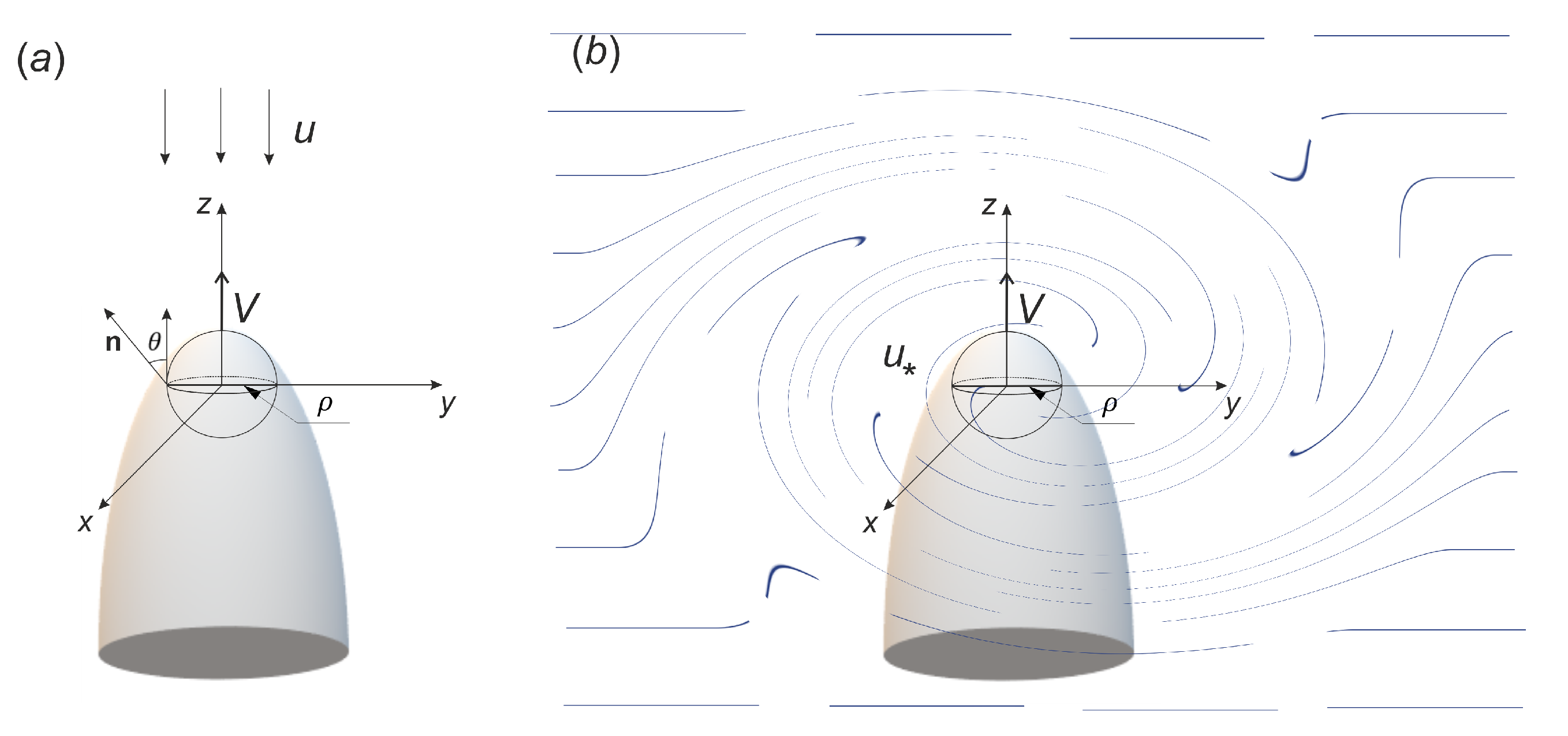
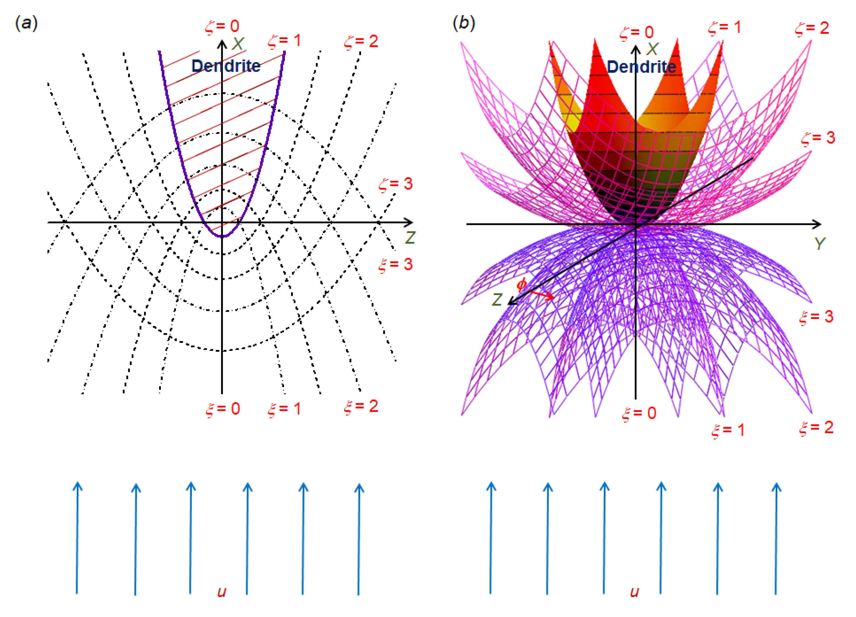
2. The Heat and Mass Transfer Model of Dendritic Growth

For simplicity, we first consider the steady-state growth of a dendritic crystal in an undercooled binary melt illustrated in Figure 1. The heat-transfer and diffusion equations in the solid and melt phases read as

$$\begin{array}{c}\hfill \frac{\partial {\theta }_s}{\partial \tau }=D_{\theta }\Delta {\theta }_s\left(\mathrm{solid}\mathrm{phase}\right),\end{array}$$

(1)

$$\begin{array}{c}\hfill \frac{\partial {\theta }_l}{\partial \tau }+(\mathbf{v}·\nabla ){\theta }_l=D_{\theta }\Delta {\theta }_l,\frac{\partial \sigma }{\partial \tau }+(\mathbf{v}·\nabla )\sigma =D_{\sigma }\Delta \sigma \left(\mathrm{liquid}\mathrm{phase}\right),\end{array}$$

(2)

where ${\theta }_s$ and ${\theta }_l$ are the temperatures in solid and liquid, $\sigma$ is the solute concentration in melt, $\tau$ is the time, $D_{\theta }$ is the temperature conductivity coefficient, $D_{\sigma }$ is the diffusivity coefficient, $\mathbf{v}$ is the velocity of oncoming melt, ∇ is the nabla operator, and $\Delta$ is the Laplacian.

We consider the viscous melt model in the Oseen hydrodynamic approximation [19,20,21], as the more general Navier–Stokes model has no analytical solutions.

$$\begin{array}{c}\hfill u\frac{\partial \mathbf{v}}{\partial z}=-\frac{1}{{\rho }_m}\nabla p+\mu \Delta \mathbf{v},\nabla ·\mathbf{v}=0,\left(\mathrm{liquid}\mathrm{phase}\right),\end{array}$$

(3)

where u is the flow velocity far from the crystal at $z\to \infty$, z is the spatial coordinate corresponding to the direction of dendrite growth, ${\rho }_m$ is the melt density, p is the hydrodynamic pressure, and $\mu$ is the kinematic viscosity. Note that the last equation in (3) describes the incompressible fluid model.

The system of hydrodynamic Equation (3) must be supplemented with appropriate boundary conditions for fluid adhesion to the dendrite surface. Since the hydrodynamic problem about the flow of a viscous melt around a dendrite does not depend on the thermal and concentration distributions, but is an independent one, below we use its solution constructed in Refs. [22,23].

Considering the case of plane-parallel melt flow far from the dendrite, we fix temperature ${\theta }_{\infty }$ and solute concentration ${\sigma }_{\infty }$ far from the growing crystal, i.e.,

$$\begin{array}{c}\hfill {\theta }_l\to {\theta }_{\infty },\sigma \to {\sigma }_{\infty }\left(\mathrm{far}\mathrm{from}\mathrm{the}\mathrm{crystal}\right).\end{array}$$

(4)

Below, we consider two possible regimes of melt flow around the growing crystal. The first of them occurs in slow laminar currents when thermal and mass fluxes are described by classical Fourier’s laws. Dealing with this case, we have

$$\begin{array}{c}\hfill \mathbf{V}·\mathbf{n}=\frac{D_{\theta }{\kappa }_p}{Q}\left(\nabla {\theta }_s-\nabla {\theta }_l\right)·\mathbf{n},(1-k_e)\sigma \mathbf{V}·\mathbf{n}=-D_{\sigma }\nabla \sigma ·\mathbf{n}\left(\mathrm{at}\mathrm{the}\mathrm{interface}\right),\end{array}$$

(5)

where V stands for the growth rate of solid/liquid interface, ${\kappa }_p$ is the specific heat, Q is the latent heat parameter, and $k_e$ is the equilibrium segregation coefficient.

The second regime occurs in cases of intense hydrodynamic currents near the solid/liquid surface of a dendrite. If this is really the case, the heat and mass fluxes become of convective-type and boundary conditions read as [24,25,26,27,28]

$$\begin{array}{c}\hfill \frac{{\theta }_Q}{D_{\theta }}\mathbf{V}·\mathbf{n}=\nabla {\theta }_s·\mathbf{n}+\frac{{\alpha }_{\theta }{\rho }_m{\kappa }_p{u}_{*}}{{\lambda }_s}({\theta }_i-{\theta }_{\infty }),\left(\mathrm{at}\mathrm{the}\mathrm{interface}\right)\\ \hfill (1-k_e){\sigma }_i\mathbf{V}·\mathbf{n}={\alpha }_{\sigma }{u}_{*}({\sigma }_i-{\sigma }_{\infty }),\left(\mathrm{at}\mathrm{the}\mathrm{interface}\right),\end{array}$$

(6)

where ${\theta }_Q=Q/{\kappa }_p$ is the adiabatic temperature, ${\alpha }_{\theta }$ and ${\alpha }_{\sigma }$ are the convective heat and mass coefficients, and ${\lambda }_s$ is the temperature conductivity in the solid. The friction velocity $u_{*}$, defining the intensity of flow near the dendrite, can be expressed in terms of shear stress $s_s$ as $u_{*}={(s_s/{\rho }_m)}^{1/2}$ [29]. In addition, the ratio of convective heat and mass coefficients is expressed as ${\alpha }_{\theta }/{\alpha }_{\sigma }={(D_{\theta }/D_{\sigma })}^{\overline{n}}$, $2/3<\overline{n}<4/5$ [24,30,31,32,33].

The last boundary condition defines the interfacial temperature in the form of

$$\begin{array}{c}\hfill {\theta }_s={\theta }_l={\theta }_{*}-m_e\sigma -{\theta }_{Q}d\mathcal{K}-\tilde{\beta }\mathbf{V}·\mathbf{n},\left(\mathrm{at}\mathrm{the}\mathrm{interface}\right),\end{array}$$

(7)

where ${\theta }_{*}$ is the phase transition temperature for a single-component melt ($\sigma =0$), $m_e$ is the equilibrium liquidus line slope, and d and $\tilde{\beta }$ stand for the capillary length and kinetic coefficient, which due to the anisotropic growth, are the functions of polar angle $\theta$ [34] shown in Figure 1

$$\begin{array}{c}\hfill d\left(\theta \right)=d_0\left\{1-{\chi }_{d}cos\left[n(\theta -{\theta }_d)\right]\right\},\tilde{\beta }\left(\theta \right)={\beta }_0{\theta }_Q\left\{1-{\chi }_{\beta }cos\left[n(\theta -{\theta }_{\beta })\right]\right\}.\end{array}$$

(8)

Here, $d_0$ and ${\beta }_0$ are the constant factors. Note that expressions (8) work in the case of n-fold dendritic symmetry. The constants ${\chi }_d$ and ${\chi }_{\beta }$ are assumed to be much smaller than unity. It is also significant to note that the crystal curvature $\mathcal{K}$ equates to $2/\rho$ and $4/\rho$ in the 2D and 3D geometries, respectively. Here, $\rho$ stands for the dendrite tip diameter. Following papers [14,18] we assume that the misalignment angles ${\theta }_d$ and ${\theta }_{\beta }$ are negligibly small.

It is convenient to solve the model (1)–(8) using special curvilinear coordinate systems (Figure 2). So, we use the parabolic cylinder reference frame in the 2D case and paraboloid of revolution reference frame in the 3D case. These curvilinear coordinates are introduced as follows

$$\begin{array}{c}\hfill z=\rho \frac{\zeta -\xi }{2},x=\rho \sqrt{\xi \zeta }\mathrm{in}2\mathrm{D},\\ \hfill z=\rho \frac{\zeta -\xi }{2},x=\rho \sqrt{\xi \zeta }cos\varphi ,y=\rho \sqrt{\xi \zeta }sin\varphi \mathrm{in}3\mathrm{D}.\end{array}$$

(9)

Here, $\rho$ represents the dendrite tip radius, and x, y, and z are the Cartesian coordinates. The coordinate $\zeta =1$ is introduced to be constant at the crystal surface and the surfaces $\zeta =const$ represent isothermal (isoconcentration) surfaces surrounding the growing dendrite.

Rewriting the model (1)–(8) in the coordinates (9) and considering that ${\theta }_l={\theta }_l\left(\zeta \right)$ and $\sigma =\sigma \left(\zeta \right)$ (the temperature ${\theta }_s$ in the solid phase is fixed), we obtain the steady-state solutions in the form of

$$\begin{array}{c}\hfill {\theta }_l\left(\zeta \right)={\theta }_i+({\theta }_{\infty }-{\theta }_i)\frac{I_{\theta }\left(\zeta \right)}{I_{\theta }(\infty )},\sigma \left(\zeta \right)={\sigma }_i+({\sigma }_{\infty }-{\sigma }_i)\frac{I_{\sigma }\left(\zeta \right)}{I_{\sigma }(\infty )}.\end{array}$$

(10)

Here, ${\theta }_i$ and ${\sigma }_i$ are the temperature and solute concentration at the dendrite surface $\zeta =1$, and $I_{\theta }\left(\zeta \right)$ and $I_{\sigma }\left(\zeta \right)$ are the temperature and concentration integrals. These functions depend on the heat and mass transfer mechanism (conductive or convective) near the crystal and are given in Section 3.1 and Section 3.2.

3. The Total Undercooling Balance

The undercooling is a measure of the deviation of the temperature at any point of a system from the equilibrium temperature of phase co-existence. The full and experimentally measurable undercooling is a sum of a number of processes: heat and mass transport in the bulk and at the interface as well as the solid–liquid interface stability due to interface energy and attachment of particles (atoms, molecules, or clusters) to the interface. All these contributions give their own influence on the growth kinetics that is expressed by the following undercooling balance.

The melt undercooling $\Delta \theta ={\theta }_{*}-{\theta }_{\infty }-m_e{\sigma }_{\infty }$ represents the driving force of dendritic growth and is given by the following terms

$$\begin{array}{c}\hfill \Delta \theta =\Delta {\theta }_{\theta }+\Delta {\theta }_{\sigma }+\Delta {\theta }_{\rho }+\Delta {\theta }_k,\end{array}$$

(11)

where $\Delta {\theta }_{\theta }$ is the thermal undercooling, $\Delta {\theta }_{\sigma }$ is the concentration undercooling, $\Delta {\theta }_{\rho }$ is the undercooling connected with the curved phase transition interface, and $\Delta {\theta }_k$ is the kinetic undercooling. The first two of them are substantially dependent on the heat and mass transfer mechanism at the dendrite interface. The last two contributions are only dependent on dendrite tip diameter $\rho$ and tip velocity V.

So, $\Delta {\theta }_{\rho }$ is given by

$$\begin{array}{c}\hfill \Delta {\theta }_{\rho }\left(\rho \right)=\frac{2d_0{\theta }_Q}{\rho }\left(2\mathrm{D}\right)\mathrm{and}\Delta {\theta }_{\rho }\left(\rho \right)=\frac{4d_0{\theta }_Q}{\rho }\left(3\mathrm{D}\right).\end{array}$$

(12)

The kinetic undercooling $\Delta {\theta }_k$ reads as

$$\begin{array}{c}\hfill \Delta {\theta }_k\left(V\right)={\left(\frac{V}{{\nu }_k}\right)}^j,\end{array}$$

(13)

where ${\nu }_k$ represents the kinetic coefficient and j is the constant derived from experimental data or numerical calculations.

3.1. Conductive Heat and Mass Transfer

Dealing with conductive heat and mass transfer near the dendritic surface, we come to the following thermal and concentration undercoolings [13,18]

$$\begin{array}{c}\hfill \Delta {\theta }_{\theta }(\rho ,V)={\theta }_i-{\theta }_{\infty }={\theta }_Q{\mathrm{Iv}}_{\theta }^{*}(\rho ,V),\\ \hfill \Delta {\theta }_{\sigma }(\rho ,V)=m_e({\sigma }_i-{\sigma }_{\infty })=\frac{m_e{\sigma }_{\infty }(1-k_e){\mathrm{Iv}}_{\sigma }^{*}(\rho ,V)}{1-(1-k_e){\mathrm{Iv}}_{\sigma }^{*}(\rho ,V)},\end{array}$$

(14)

where the modified (thermal and concentration) Ivantsov functions take the form

$${\mathrm{Iv}}_{\theta }^{*}(\rho ,V)=P_{\theta }(\rho ,V)exp\left[P_0(\rho ,V)\right]I_{\theta }(\infty ),$$

$${\mathrm{Iv}}_{\sigma }^{*}(\rho ,V)=P_{\theta }(\rho ,V)\frac{D_{\theta }}{D_{\sigma }}exp\left[\frac{P_0(\rho ,V)D_{\theta }}{D_{\sigma }}\right]I_{\sigma }(\infty ).$$

Here, the thermal ($P_{\theta }$) and flow ($P_u$) Péclet numbers are defined as

$$P_{\theta }(\rho ,V)=\frac{\rho V}{2D_{\theta }},P_u\left(\rho \right)=\frac{\rho u}{2D_{\theta }}\mathrm{and}{P}_0(\rho ,V)=P_{\theta }(\rho ,V)+P_u\left(\rho \right).$$

The interfacial temperature ${\theta }_i$ and solute concentration ${\sigma }_i$, as well as the integrals $I_{\theta }$ and $I_{\sigma }$, are given by [13,18]

$${\theta }_i={\theta }_{\infty }+{\theta }_Q{P}_{\theta }exp\left(P_0\right)I_{\theta }(\infty ),$$

$${\sigma }_i=\frac{{\sigma }_{\infty }}{1-(1-k_e)exp(P_0{D}_{\theta }/D_{\sigma })P_{\theta }{I}_{\sigma }(\infty )D_{\theta }/D_{\sigma }},$$

$$I_{\theta }\left(\zeta \right)=\underset{1}{\overset{\zeta }{\int }}exp\left[(k-1)P_u\underset{1}{\overset{{\zeta }_1}{\int }}\frac{G\left({\zeta }_2\right)d{\zeta }_2}{\sqrt{{\zeta }_2}}-P_0{\zeta }_1\right]\frac{d{\zeta }_1}{{\zeta }_1^{(k-1)/2}},$$

$$I_{\sigma }\left(\zeta \right)=\underset{1}{\overset{\zeta }{\int }}exp\left[(k-1)P_u\frac{D_{\theta }}{D_{\sigma }}\underset{1}{\overset{{\zeta }_1}{\int }}\frac{G\left({\zeta }_2\right)d{\zeta }_2}{\sqrt{{\zeta }_2}}-P_0\frac{D_{\theta }}{D_{\sigma }}{\zeta }_1\right]\frac{d{\zeta }_1}{{\zeta }_1^{(k-1)/2}},$$

where $k=2$ and $k=3$ in cases of the 2D and 3D dendritic geometry.

The function $G\left(\zeta \right)$ entering these expressions is determined from the hydrodynamic solution of the Oseen viscous flow model and is given by [22,23] in the 2D and 3D cases

$$G\left(\zeta \right)=\frac{\sqrt{2}}{\sqrt{\pi \Re }\mathrm{erfc}\sqrt{\Re /2}}\left[exp\left(-\frac{\Re }{2}\right)-exp\left(-\frac{\zeta \Re }{2}\right)\right]+\frac{\mathrm{erfc}\sqrt{\zeta \Re /2}}{\mathrm{erfc}\sqrt{\Re /2}}\sqrt{\zeta }\mathrm{in}2\mathrm{D},$$

$$G\left(\zeta \right)=\frac{exp(-\Re /2)-exp(-\zeta \Re /2)}{\sqrt{\zeta }\Re E_1(\Re /2)}+\frac{\sqrt{\zeta }{E}_1(\zeta \Re /2)}{2E_1(\Re /2)}\mathrm{in}3\mathrm{D},$$

where $\Re =\rho u/\mu$ stands for the Reynolds number, and $E_1\left(w\right)={\int }_w^{\infty }{\lambda }^{-1}exp(-\lambda )d\lambda$.

As a result, the contributions in the total undercooling balance (11) in the case of conductive heat and mass transfer mechanism are defined by expressions (12)–(14).

3.2. Convective Heat and Mass Transfer

Dealing with intense fluid motions and mixing near the dendrite surface, we come to the following temperature and concentration undercoolings for convective heat and mass transfer mechanism [18]

$$\begin{array}{c}\hfill \Delta {\theta }_{\theta }\left(V\right)={\theta }_i-{\theta }_{\infty }=\frac{{\theta }_{Q}V{\lambda }_s}{{\alpha }_{\theta }{\rho }_m{\kappa }_p{u}_{*}{D}_{\theta }},\\ \hfill \Delta {\theta }_{\sigma }\left(V\right)=m_e({\sigma }_i-{\sigma }_{\infty })=\frac{(1-k_e)V{m}_e{\sigma }_{\infty }}{{\alpha }_{\sigma }{u}_{*}-(1-k_e)V}.\end{array}$$

(15)

The integrals $I_{\theta }\left(\zeta \right)$ and $I_{\sigma }\left(\zeta \right)$ entering in (10) in the case of convective transfer mechanism are given by

$$I_{\theta }\left(\zeta \right)=\underset{1}{\overset{\zeta }{\int }}\frac{exp(-P_{\theta }{\zeta }_1)}{{\zeta }_1^{(k-1)/2}}d{\zeta }_1,I_{\sigma }\left(\zeta \right)=\underset{1}{\overset{\zeta }{\int }}\frac{exp(-P_{\sigma }{\zeta }_1)}{{\zeta }_1^{(k-1)/2}}d{\zeta }_1,P_{\sigma }=\frac{\rho V}{2D_{\sigma }},$$

and, as before, $k=2$ and $k=3$ describe the 2D and 3D growth geometries. Thus, the contributions in the total undercooling balance (11) in the case of convective heat and mass transfer mechanism are defined by expressions (12), (13) and (15).

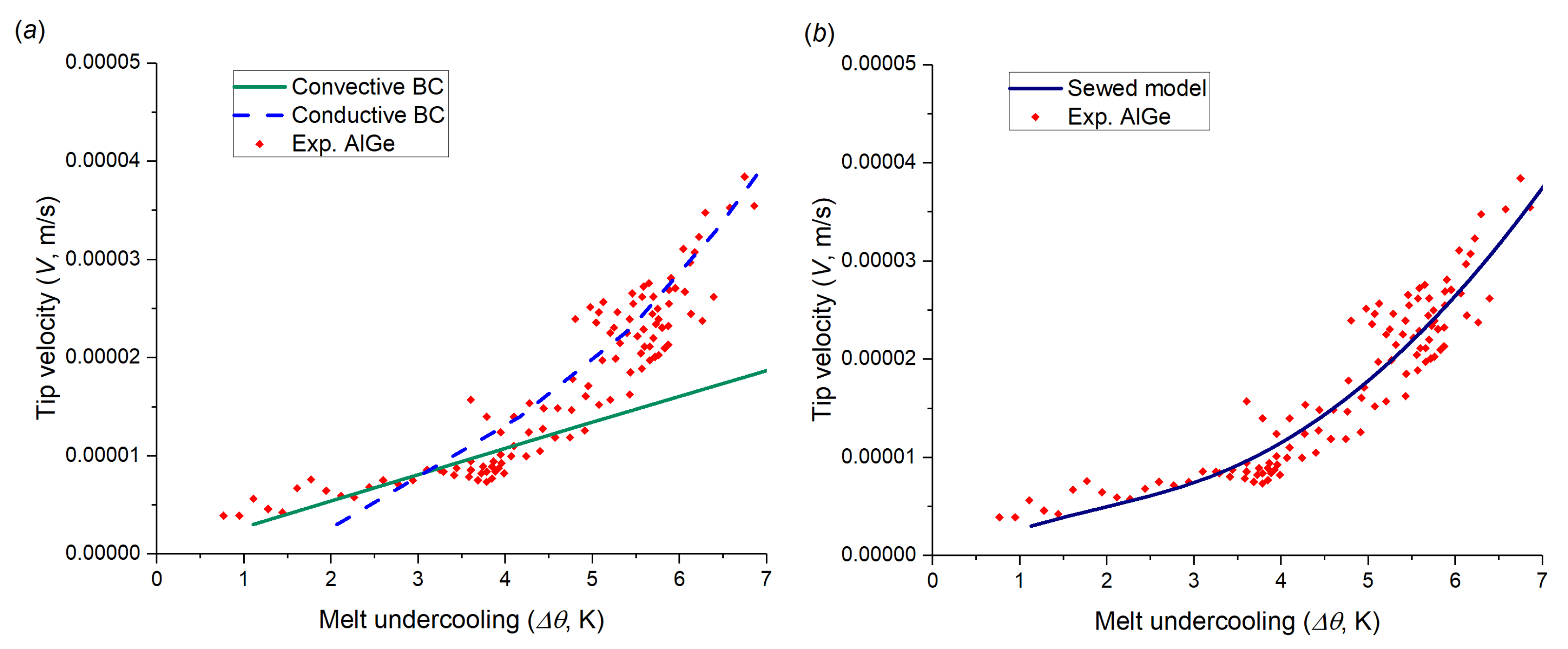
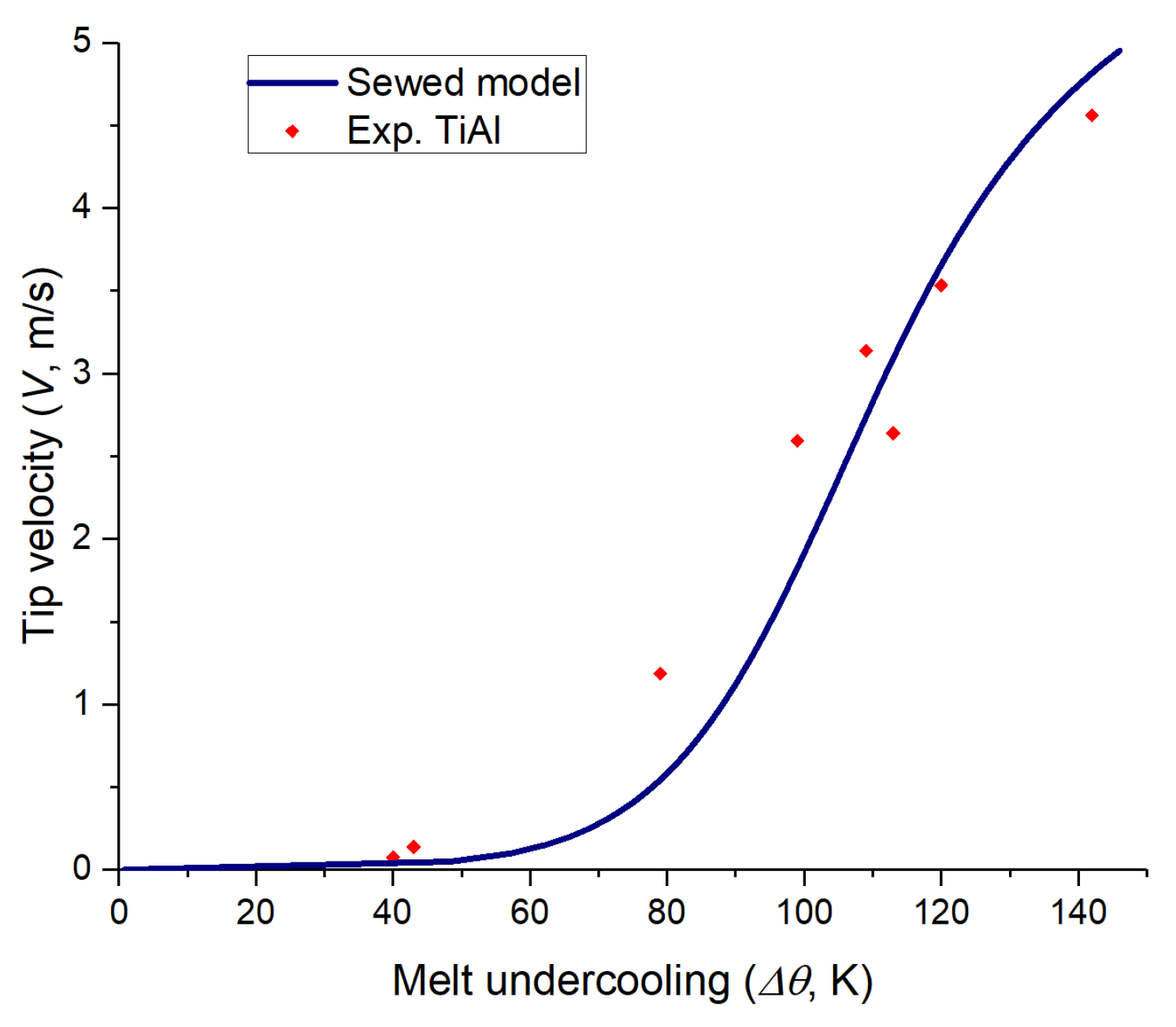
3.3. Sewing Together Undercooling Balances

In this section, we sew together the undercooling balances for conductive and convective heat and mass transfer to describe mixed transfer mechanisms near the dendritic surface. To do this, we introduce the corresponding superscripts “cond” and “conv”, i.e., we write the melt undercoolings as $\Delta {\theta }^{cond}$ for conductive mechanism and $\Delta {\theta }^{conv}$ for convective mechanism. To sew together these functions of $\Delta \theta$ let us write down the following law

$$\begin{array}{c}\hfill \Delta \theta =\Delta {\theta }_{sewed}=\frac{\Delta {\theta }^{conv}{B}^{conv}(\Delta \theta )+\Delta {\theta }^{cond}{B}^{cond}(\Delta \theta )}{B^{conv}(\Delta \theta )+B^{cond}(\Delta \theta )},\end{array}$$

(16)

where $B^{cond}(\Delta \theta )$ and $B^{conv}(\Delta \theta )$ are the sewing functions. These functions should satisfy the following limiting cases: $B^{cond}(\Delta \theta )\to 0$ for $\Delta \theta \to 0$ and $B^{conv}(\Delta \theta )\to 0$ for $\Delta \theta \gg \Delta {\theta }_c$, where $\Delta {\theta }_c$ is a characteristic undercooling (e.g., initial undercooling). In other words, $\Delta {\theta }_{sewed}\approx \Delta {\theta }^{conv}$ for small and $\Delta {\theta }_{sewed}\approx \Delta {\theta }^{cond}$ for large melt undercoolings. The sewing functions can be chosen in various ways. So, for example, when describing dendritic tip shapes, the authors of Refs. [35,36] used the exponential sewing functions. On the other hand, when describing dynamics of intracellular clusters of nanoparticles, the authors of Ref. [37] used power functions to stitch together different asymptotic solutions.

4. Selection Criterion

Equation (16) expresses $\rho$, V and $\Delta \theta$. To obtain $\rho (\Delta \theta )$ and $V(\Delta \theta )$ independently, we need one more equation between these variables. Such an equation, known as the selection criterion, follows from the solvability theory and stability analysis [13,18,34,38,39,40].

4.1. Solvability Condition

The solvability condition defines the family of solutions for temperature and solute concentration distributions lying in the vicinity of parabolic/paraboloidal Ivantsov solutions. This condition takes the form [41]

$$\begin{array}{c}\hfill \underset{-\infty }{\overset{\infty }{\int }}A\left[{\Xi }_0(\ell )\right]{\wp }_m(\ell )d\ell =0,{\wp }_m(\ell )=exp\left[i\underset{0}{\overset{\ell }{\int }}{\kappa }_m\left({\ell }_1\right)d{\ell }_1\right].\end{array}$$

(17)

Here, A represents a curvature operator, ${\kappa }_m$ is the wavenumber found from stability theory (see Section 4.2), ${\Xi }_0(\ell )$ is the solution of corresponding boundary-value problem, and i is the unit imaginary number. Equation (17) will be used below to obtain the second equation connecting $\rho$, V and $\Delta \theta$.

4.2. Conductive Heat and Mass Transfer

Now we consider the conductive-type boundary conditions at the growing dendritic surface. Following the theory [10], we expand the flow velocity components $u_{\xi }$ and $u_{\zeta }$ in series at the point $\zeta =1$ for the 2D crystal. The result reads as

$$\begin{array}{c}\hfill u_{\xi }={\left(\frac{\xi }{\xi +1}\right)}^{1/2}\left(V+b(\Re )u(\zeta -1)\right),u_{\zeta }=-V{(\xi +1)}^{-1/2},\end{array}$$

(18)

where

$$b(\Re )={\left(\frac{\Re }{2\pi }\right)}^{1/2}\frac{exp(-\Re /2)}{\mathrm{erfc}\left(\sqrt{\Re /2}\right)}\mathrm{in}2\mathrm{D}\mathrm{and}b(\Re )=\frac{exp(-\Re /2)}{E_1(\Re /2)}\mathrm{in}3\mathrm{D}.$$

Again, following the theory [10], we use the local Cartesian reference frame ($x_l,y_l$) fixed at the dendrite surface and shifting together with the crystal. Keeping this in mind, we rewrite Formulas (18) as (here the axes $x_l$ and $y_l$ point out the tangent and normal directions)

$$\begin{array}{c}\hfill \tilde{u}=-y_l\frac{b(\Re )u}{2\rho }sin\left(2\theta \right)-Vsin\theta ,\tilde{v}=-Vcos\theta ,\end{array}$$

(19)

where $\tilde{u}$ and $\tilde{v}$ represent the tangent and normal velocities near dendritic surface.

The boundary conditions (5) determine the following derivatives at the solid/liquid surface $y_l=0$

$$\begin{array}{c}\hfill \frac{d{\tilde{\theta }}_l}{d{y}_l}=-\frac{{\theta }_{Q}Vcos\theta }{D_{\theta }},\frac{d\tilde{\sigma }}{d{y}_l}=\frac{(k_e-1)V{\sigma }_{i}cos\theta }{D_{\sigma }},y_l=0.\end{array}$$

(20)

Here, and below the “tilde” above, the symbols indicate the steady-state solutions. Keeping this in mind, we have the temperature and solute concentration near the solid/liquid surface

$$\begin{array}{c}\hfill {\tilde{\theta }}_l={\theta }_i-y_l\frac{{\theta }_{Q}Vcos\theta }{D_{\theta }},\tilde{\sigma }={\sigma }_i+y_l\frac{(k_e-1)V{\sigma }_{i}cos\theta }{D_{\sigma }}.\end{array}$$

(21)

To find the wavenumber ${\kappa }_m$ in (17), we perturb the steady-state solutions of (i) fluid flow near the growing dendrite as $u^{\prime }$ and $v^{\prime }$, (ii) temperature field in the solid and liquid phases as ${\theta }_s^{\prime }$ and ${\theta }_l^{\prime }$, (iii) solute concentration in liquid as ${\sigma }^{\prime }$, (iv) hydrodynamic pressure as $p^{\prime }$, and (v) solid/liquid interface as ${\Sigma }^{\prime }$. All perturbations are assumed to be small compared to the corresponding steady-state functions. Equations governing a behaviour of perturbations follow from (1)–(3) and take the form

$$\begin{array}{c}\hfill \frac{\partial {\theta }_s^{\prime }}{\partial \tau }+\tilde{u}\frac{\partial {\theta }_s^{\prime }}{\partial x_l}+\tilde{v}\frac{\partial {\theta }_s^{\prime }}{\partial y_l}+v^{\prime }\frac{d{\tilde{\theta }}_s}{d{y}_l}=D_{\theta }\Delta {\theta }_s^{\prime },\\ \hfill \frac{\partial {\theta }_l^{\prime }}{\partial \tau }+\tilde{u}\frac{\partial {\theta }_l^{\prime }}{\partial x_l}+\tilde{v}\frac{\partial {\theta }_l^{\prime }}{\partial y_l}+v^{\prime }\frac{d{\tilde{\theta }}_l}{d{y}_l}=D_{\theta }\Delta {\theta }_l^{\prime },\\ \hfill \frac{\partial {\sigma }^{\prime }}{\partial \tau }+\tilde{u}\frac{\partial {\sigma }^{\prime }}{\partial x_l}+\tilde{v}\frac{\partial {\sigma }^{\prime }}{\partial y_l}+v^{\prime }\frac{d\tilde{\sigma }}{d{y}_l}=D_{\sigma }\Delta {\sigma }^{\prime },\\ \hfill \nabla p^{\prime }=\mu {\rho }_m\Delta {\mathbf{v}}^{\prime },\nabla ·{\mathbf{v}}^{\prime }=0.\end{array}$$

(22)

Here, ${\mathbf{v}}^{\prime }$ means the vector of hydrodynamic perturbations.

Expanding expressions (5) and (7) in series near dendrite surface $y_l=0$, we arrive at

$$\begin{array}{c}\hfill {\theta }_s^{\prime }+{\theta }_l^{\prime }-\frac{{\theta }_{Q}Vcos\theta }{D_{\theta }}{\Sigma }^{\prime }=0,\\ \hfill {\theta }_s^{\prime }-{\theta }_{Q}d\left(\theta \right)\frac{{\partial }^2{\Sigma }^{\prime }}{\partial y_l^2}+\tilde{\beta }\left(\theta \right)\frac{\partial {\Sigma }^{\prime }}{\partial \tau }-m_e{\sigma }^{\prime }+\frac{m_e{\sigma }_i(1-k_e)Vcos\theta }{D_{\sigma }}{\Sigma }^{\prime }=0,\\ \hfill u^{\prime }=0,v^{\prime }+\frac{\partial {\Sigma }^{\prime }}{\partial \tau }=0,\frac{{\theta }_Q}{D_{\theta }}\frac{\partial {\Sigma }^{\prime }}{\partial \tau }-\frac{\partial {\theta }_s^{\prime }}{\partial y_l}+\frac{\partial {\theta }_l^{\prime }}{\partial y_l}+\frac{{\theta }_Q{V}^2{cos}^2\theta }{D_{\theta }^2}{\Sigma }^{\prime }=0.\end{array}$$

(23)

Let us especially underline that all perturbations are proportional to

$$\begin{array}{c}\hfill exp\left(\varpi \tau +i\kappa x_l-\epsilon \kappa y_l\right)\end{array}$$

(24)

within the framework of linear stability theory (see, among others, [10,13,18]). Here, $\varpi$ and $\kappa$ stand for the frequency and wavenumber of perturbations, and $\left|\epsilon \right|=1$ defines the convergence of perturbations for $y_l\to \infty$.

The method for constructing the analytical expressions for perturbations is described in detail in several papers devoted to the morphological stability theory (see, among others, [10,13,18]). Therefore, to save room, we mention only the main idea for finding such solutions. Considering all perturbations to be proportional to the exponential function (24), we find equations for their amplitudes from the boundary conditions (23). Then, to obtain a nontrivial solution for a system of linear equations for such amplitudes, we equate the determinant of this linear system to zero and come to the following cubic equation for the wavenumber $\kappa ={\kappa }_m$

$$\begin{array}{c}\hfill {\kappa }_m^3-{\kappa }_m\left(\frac{V}{2D_{\theta }d\left(\theta \right)}+\frac{m_e(1-k_e){\sigma }_{i}V}{{\theta }_Q{D}_{\sigma }d\left(\theta \right)}\right)exp\left(i\theta \right)-i{\kappa }_m\frac{b(\Re )usin\left(2\theta \right)}{16\rho D_{\theta }}\\ \hfill -i{\kappa }_m\frac{b(\Re )usin\left(2\theta \right)}{8\rho D_{\sigma }}+i{\kappa }_m^2\frac{Vsin\theta }{2D_{\theta }}-\frac{V^{2}cos\theta exp\left(i\theta \right)}{4D_{\theta }^{2}d\left(\theta \right)}-i{\kappa }_m^2\frac{\tilde{\beta }\left(\theta \right)Vsin\theta }{{\theta }_{Q}d\left(\theta \right)}=0.\end{array}$$

(25)

In deriving Equation (25), it was taken into account that the moving coordinate system associated with the dendrite tip is travelling in space at velocity $-i\kappa Vsin\theta$. As this takes place, the perturbation evolves with the velocity $\varpi \left(\kappa \right)$. Therefore, the real velocity of a perturbation represents the sum of these velocities and looks like $\varpi \left(\kappa \right)-iV\kappa sin\theta$. Again, let us mention that the growth rate V of the dendritic tip is assumed to be constant throughout this paper. Here, we refer the interested reader to the theory [42] of how fast the dendrite reaches its steady-state velocity V. Furthermore, we have considered the neutral stability surface, where $\kappa ={\kappa }_m$ ($\varpi =0$), put $\epsilon =-1$, and changed i by $-i$ accordingly to the theory of Ref. [10]. An important point is that expression (25) corresponds to previously developed theories [8,9,10,13,41,43,44,45,46,47] in various limiting cases.

Next, combining (17) and (25), we get the selection criterion for conductive heat and mass transfer boundary conditions

$$\begin{array}{c}\hfill {\sigma }^{*cond}\equiv 2d_0{D}_{\theta }{\rho }^{-2}{V}^{-1}=\frac{{\sigma }_{0n}{\chi }_d^{7/n}{B}_n^{7/n}}{1+\beta {\overline{\nu }}_n^{s_n}}\left\{\frac{1}{{\left[1+b_{1n}{\chi }_d^{2/n}{B}_n^{2/n}{P}_{\theta }\left(1+{\Delta }_0{\beta }_0{D}_{\theta }/d_0\right)\right]}^2}\right.\\ \hfill +\left.\frac{2m_e(1-k_e){\sigma }_i{D}_{\theta }}{{\left[1+b_{2n}{\chi }_d^{2/n}{B}_n^{2/n}{P}_{\sigma }\left(1+{\Delta }_0{\beta }_0{D}_{\sigma }/d_{0CD}\right)\right]}^2{D}_{\sigma }{\theta }_Q}\right\},\end{array}$$

(26)

where

$${\overline{\nu }}_n={\chi }_d^{-3/n}{B}_n^{-3/n}\left(\frac{b(\Re )u{d}_0}{4V\rho R}+\frac{b(\Re )u{d}_0{D}_{\theta }}{2V\rho R{D}_{\sigma }}\right),s_n=\frac{7+n}{2(3+n)},R=1+\frac{2m_e(1-k_e){\sigma }_i{D}_{\theta }}{D_{\sigma }{\theta }_Q},$$

$$d_{0CD}=\frac{d_0{\theta }_Q}{2m_e(1-k_e){\sigma }_i},B_n=\frac{1}{2^{3n/4}}\sum _{j=0}^n\left(\genfrac{}{}{0pt}{}{n}{j}\right)i^{n-j}cos\frac{\pi (n-j)}{2},$$

$$b_{1n}={\left(\frac{8{\sigma }_{0n}}{7}\right)}^{1/2}{\left(\frac{3}{56}\right)}^{3/8}{B}_n^{3/2n}{\chi }_d^{3/2n-3/8},b_{2n}=\sqrt{2}{b}_{1n},{\Delta }_0=20{\left(\frac{7}{24}\right)}^{1/2}{\left(\frac{56}{3}\right)}^{3/8}.$$

Here, ${\sigma }_{0n}$ and $\beta$ are the selection constants. The first of them defines the stable mode of dendritic growth in the absence of hydrodynamic flow, whereas the second one is responsible for hydrodynamic flows. The selection criterion (26) determines the second equation connecting $\rho$, V and $\Delta \theta$ for conductive heat and mass transfer boundary conditions. Now, coupling (11) and (26), one can find the functions $\rho (\Delta \theta )$ and $V(\Delta \theta )$. Note that criterion (26) has limiting transitions to previously developed theories [8,9,10,13,41,43,44,45,46,47]. The theory developed can be used for the three-dimensional dendritic growth as well. In this case, we have to replace the solution of the two-dimensional heat and mass transfer and hydrodynamic equations with the corresponding three-dimensional solutions. Therefore, the system (11) and (26) works in the 3D case too.

4.3. Convective Heat and Mass Transfer

Now, we consider the convective-type boundary conditions at the growing dendritic surface. In this case, the theory considered in Section 4.2 should be modified. At first, now expressions (19) look like $\tilde{u}=-Vsin\theta$ and $\tilde{v}=-Vcos\theta$. The boundary conditions (23) become

$$\begin{array}{c}\hfill {\theta }_l^{\prime }+(f_1+m_e{f}_2){\Sigma }^{\prime }+m_e{\sigma }^{\prime }+d{\theta }_Q\frac{{\partial }^2{\Sigma }^{\prime }}{\partial y_l^2}-\tilde{\beta }\frac{\partial {\Sigma }^{\prime }}{\partial \tau }=0,\\ \hfill {\theta }_s^{\prime }-m_e{f}_2{\Sigma }^{\prime }-m_e{\sigma }^{\prime }-d{\theta }_Q\frac{{\partial }^2{\Sigma }^{\prime }}{\partial y_l^2}+\tilde{\beta }\frac{\partial {\Sigma }^{\prime }}{\partial \tau }=0,\\ \hfill \frac{{\theta }_Q}{D_{\theta }}\frac{\partial {\Sigma }^{\prime }}{\partial \tau }-\frac{\partial {\theta }_s^{\prime }}{\partial y_l}+2h{f}_1{\Sigma }^{\prime }+2h{\theta }_l^{\prime },\\ \hfill \frac{1-k_e}{{\alpha }_{\sigma }{u}_{*}}\left[Vcos\theta ({\sigma }^{\prime }+f_2{\Sigma }^{\prime })+{\sigma }_i\frac{\partial {\Sigma }^{\prime }}{\partial \tau }\right]+{\sigma }^{\prime }+f_2{\Sigma }^{\prime }=0,\end{array}$$

(27)

where $h={\alpha }_{\theta }{\rho }_m{\kappa }_p{u}_{*}/\left(2{\lambda }_s\right)$.

Equating to zero the determinant of coefficients at perturbations following from Equation (27), we obtain the marginal mode of the wavenumber

$$\begin{array}{c}\hfill {\kappa }_m^2+{\kappa }_m\left(2h-i\frac{\tilde{\beta }Vsin\theta }{{\theta }_{Q}d}-i\frac{Y_{2}sin\theta }{Y_{1}d}\right)-i\frac{2h\tilde{\beta }Vsin\theta }{{\theta }_{Q}d}-i\frac{Vsin\theta }{D_{\theta }d}-i\frac{2h{Y}_{2}sin\theta }{Y_{1}d}=0,\end{array}$$

(28)

where

$$Y_1=1+\frac{(1-k_e)Vcos\theta }{{\alpha }_{\sigma }{u}_{*}},Y_2=\frac{(1-k_e)m_e{\sigma }_{i}V}{{\alpha }_{\sigma }{\theta }_Q{u}_{*}}.$$

Now, combining (17) and (28), we get the selection criterion for convective heat and mass transfer boundary conditions

$$\begin{array}{c}\hfill {\sigma }^{*conv}\equiv 2d_0{D}_{\theta }{\rho }^{-2}{V}^{-1}=\frac{2{\sigma }_{0n}^c{\chi }_d^{2/n}{B}_n^{2/n}{D}_{\theta }{\beta }_1}{\rho }\\ \hfill +\frac{{\sigma }_{0n}^c{\chi }_d^{5/n}{B}_n^{5/n}\left(1+b_1{\beta }_1{D}_{\theta }\right){\left[1+r_n{\tilde{\nu }}_{1n}^{(n+5)/2(n-1)}\right]}^2}{{\left[1+l_n\left({\chi }_d^{3/n}{B}_n^{3/n}{b}_1\rho +3{\chi }_d^{1/4}{B}_n^{2/n}{P}_{\theta }{D}_{\theta }{\beta }_1/\left(2^{1/4}{d}_0\right)\right)\right]}^2},\end{array}$$

(29)

where

$$b_1=\frac{{\alpha }_{\theta }{u}_{*}{\rho }_m{\kappa }_p}{2{\lambda }_s},{\beta }_1={\beta }_0+\frac{m_e(1-k_e){\sigma }_i}{{\alpha }_{\sigma }{u}_{*}{\theta }_Q},l_n^2=2^{9/2}\frac{25}{27}{\sigma }_{0n}^c,{\tilde{\nu }}_{1n}=\frac{b_1^2{\chi }_d^{1/n}{B}_n^{1/n}\rho d_0}{2^{1/4}{P}_{\theta }(1+b_1{\beta }_1{D}_{\theta })}.$$

Here, ${\sigma }_{0n}^c$ and $r_n$ represent selection constants dependent on the crystalline symmetry (subscript n).

The selection criterion (29) defines the second equation connecting $\rho$, V and $\Delta \theta$ for convective heat and mass-transfer boundary conditions. Now, coupling (11) and (29), one can find the functions $\rho (\Delta \theta )$ and $V(\Delta \theta )$. As before, the theory developed can be used for the three-dimensional dendritic growth as well.

4.4. Sewing Together Selection Criteria

Let us now sew together selection criteria (26) and (29) for conductive and convective heat and mass transfer near a dendrite surface

$$\begin{array}{c}\hfill {\sigma }_{sewed}^{*}=\frac{{\sigma }^{*conv}{B}^{conv}(\Delta \theta )+{\sigma }^{*cond}{B}^{cond}(\Delta \theta )}{B^{conv}(\Delta \theta )+B^{cond}(\Delta \theta )}.\end{array}$$

(30)

As before, ${\sigma }_{sewed}^{*}\approx {\sigma }^{*conv}$ for smaller and ${\sigma }_{sewed}^{*}\approx {\sigma }^{*cond}$ for larger melt undercoolings.This means that criterion (30) contains limiting transitions to the conductive and convective mechanisms of heat and mass transfer. If both mechanisms take place simultaneously, we have two nonlinear Equations (16) and (30) to find $\rho (\Delta \theta )$ and $V(\Delta \theta )$. An important point is that these equations should describe both undercooling limits: low $\Delta \theta$ (convective mechanism prevails) and moderate $\Delta \theta$ (conductive mechanism prevails). Note that a behaviour of $\rho (\Delta \theta )$ and $V(\Delta \theta )$ will substantially depend on the sewing functions $B^{cond}(\Delta \theta )$ and $B^{conv}(\Delta \theta )$, which can be chosen in different ways [35,36,37,48,49]. The essential conditions are only those $B^{cond}(\Delta \theta )\to 0$ for $\Delta \theta \to 0$ and $B^{conv}(\Delta \theta )\to 0$ for $\Delta \theta \gg \Delta {\theta }_c$. In the next section, we analyse the sewed solutions (16) and (30) for different undercooled melts.

5. Behaviour of Sewed Functions

First of all, let us choose the stitching functions entering in the sewed undercooling balance (16) and selection criterion (30). Following previous studies [35,36,37], we chose power functions as follows

$$\begin{array}{c}\hfill B^{conv}(\Delta \theta )={ϵ}_{conv}{\left(\frac{{\theta }_Q}{\Delta \theta }\right)}^{j_{conv}},B^{cond}(\Delta \theta )={ϵ}_{cond}{\left(\frac{\Delta \theta }{{\theta }_{*}}\right)}^{j_{cond}}.\end{array}$$

(31)

Here, ${ϵ}_{conv}$ and ${ϵ}_{cond}$ are the stitching constants, and $j_{conv}\ge 1$ and $j_{cond}\ge 1$ are the parameters determining the smoothness of stitching functions. These values should also provide the correct behaviour of $B^{conv}(\Delta \theta )$ and $B^{cond}(\Delta \theta )$ for small and large melt undercoolings. Namely, $B^{conv}(\Delta \theta )\to 0$ at large $\Delta \theta$ ($\Delta \theta \gg {\theta }_Q$) and $B^{cond}(\Delta \theta )\to 0$ at small $\Delta \theta$ ($\Delta \theta \ll {\theta }_{*}$). Taking these limiting cases into account, we see that

$$\Delta \theta \approx \Delta {\theta }^{conv}\mathrm{and}{\sigma }^{*}\approx {\sigma }^{*conv},\mathrm{small}\mathrm{undercooling},$$

$$\Delta \theta \approx \Delta {\theta }^{cond}\mathrm{and}{\sigma }^{*}\approx {\sigma }^{*cond},\mathrm{large}\mathrm{undercooling}.$$

Such behaviour provides a correct smooth transition of the sewed solution compared with purely convective and conductive branches shown in Figure 3 for the Al${}_{24}$Ge${}_{76}$ melt. The solidification experiments with Al${}_{24}$Ge${}_{76}$ alloy (see for details [15]) were carried out using a horizontal sample alignment, minimising gravity-induced fluid flow. The driving force for solidification is the total undercooling $\Delta \theta$ at the dendrite tip. It is determined as the sum of solutal and curvature (Gibbs–Thomson effect) undercooling; kinetic and thermal undercooling were neglected (i.e., $\Delta {\theta }_{\theta }=0$ and $\Delta {\theta }_k=0$), because fast thermal diffusion was assumed.

Comparing the theory with the experimental data, it is easy to see that each of these branches moves away from the experimental points into the region of its invalidity: the convective branch (solid line in Figure 3a) does not work for larger $\Delta \theta$, while the conductive one (dashed line in Figure 3a) does not describe experiments for smaller $\Delta \theta$. Both branches sewed together (solid line in Figure 3b) well satisfy experimental points in the whole diapason of melt undercooling.

To check the theory functionality for another system, we compare the sewed solution for the Ti${}_{45}$Al${}_{55}$ droplets processed in electromagnetic levitators [13] in Figure 4. The sewed model is able to quantitatively reproduce the experimental results obtained by Hartmann et al. (see [16]). Note that that the intensity of convection and flow velocity are not measured in experiments of [16] directly. In this sense, the theoretical model uses the fluid velocity $u_{*}$ as the parameter, which relates to the process of viscous flow in levitated droplets realistically. Thus, convective boundary conditions well describe two experimental points lying near 40 K and conductive boundary conditions covering the intermediate region, as well as the whole undercooling diapason. As is easily seen, the sewed “tip velocity—melt undercooling” curve describes both limiting regimes with smaller and larger $\Delta \theta$, as well as the intermediate regime between them. In other words, the whole diapason of experimental measurements is covered.

The reason for this behaviour, from a practical viewpoint, is that vigorous currents of liquid could occur in the vicinity of growing dendrites. This in turn is associated with a laminar-to-turbulent transition when undercooled droplets solidify in electromagnetic levitators [50]. This transition may be driven as a result of vigorous fluid swirls, resulting in a convective heat and mass transport near the surfaces of crystals. Therefore, taking all of the above into account, we conclude that convective boundary conditions might outline experimental data on melt solidification for small undercooling by analogy with ice dendrites grown in sea water [24,25,26,27].

6. Conclusions

In summary, we developed a generalised theory of stable dendritic growth in undercooled binary melts in the presence of convective flows. First of all, we considered two kinds of solidification conditions: (i) forced melt convection when conductive-type heat and mass transfer boundary conditions take place, and (ii) intense melt convection (e.g., caused by turbulent flows near the dendrite surface or various peculiarities of hydrodynamics currents) when convective-type heat and mass transfer boundary conditions occur. The first of these cases describes moderate and high melt undercoolings $\Delta \theta$, whereas the second one corresponds to smaller values of the driving force $\Delta \theta$. Let us especially underline that small driving forces $\Delta \theta$ happen at $P_{\theta }\lesssim {10}^{-3}$, moderate $\Delta \theta$ occur at ${10}^{-3}\lesssim P_{\theta }\lesssim {10}^{-2}$, and high $\Delta \theta$ correspond to $P_{\theta }\gtrsim {10}^{-2}$ [35]. Sewing together these cases, we described a wider range of melt undercoolings (both of these cases) until local-equilibrium crystallisation conditions are fulfilled. To do this, we derived undercooling balances and stability criteria for cases (i) and (ii) independently. Then these expressions were sewed together using the generalised Formulas (16) and (30), which represent the main outcome of our theory. Analysing these laws, we saw that the present solution contained two branches, convective and conductive. The first of them describes low melt undercoolings, while the second one is valid for moderate and high driving forces. The stitching functions $B^{conv}(\Delta \theta )$ and $B^{cond}(\Delta \theta )$ ensure a smooth transition between these branches. These functions can only be chosen by comparing theory and experimental data. Our simulations based on Formulas (16) and (30) demonstrated that the theory and experiments are in good agreement. Let us especially highlight in this conclusion that the stable growth mode of dendrites in local nonequilibrium crystallisation conditions $P_{\theta }\gtrsim 1$ can also be selected using the hyperbolic diffusion equation, modified mass balance condition, and nonequilibrium expressions for the segregation coefficient and liquidus line slope. Such a theory was developed in our previous studies [51,52].

Note that it is convenient to use the power laws “dendrite tip velocity—undercooling” and “dendrite tip diameter—undercooling” to compare the theory and experimental data. Such laws can be derived analytically in some limiting cases (see, among others, Ref. [46]). When studying different asymptotics to derive similar power laws for different undercoolings, Péclet and Reynolds numbers represent one of the important tasks for future investigations.

The theory under consideration could be further developed to describe the anomalous (U-shape) behaviour of the velocity–undercooling relationship found in experiments aboard the International Space Station [53]. To describe these experiments where dendritic growth and crystal nucleation occur simultaneously ahead of the recalescence front, we also need to use nucleation theory at initial and intermediate stages (see, among others, recently published papers [54,55,56,57]). This will be the subject of further investigations in the near future.

References

1. Chernov, A.A. Modern Crystallography III: Crystal Growth; Springer: Berlin, Germany, 1984. [Google Scholar]
2. Huang, S.-C.; Glicksman, M.E. Overview 12: Fundamentals of dendritic solidification—I. Steady-state tip growth. Acta Metall. 1981, 29, 701–715. [Google Scholar] [CrossRef]
3. Trivedi, R.; Kurz, W. Dendritic growth. Int. Mater. Rev. 1994, 39, 49–74. [Google Scholar] [CrossRef]
4. Galenko, P.K.; Zhuravlev, V.A. Physics of Dendrites; World Scientific: Singapore, 1994. [Google Scholar]
5. Kurz, W.; Fisher, D.J. Fundamentals of Solidification; Trans Tech Publ.: Aedermannsdorf, Switzerland, 1989. [Google Scholar]
6. Huppert, H.E. The fluid mechanics of solidification. J. Fluid Mech. 1990, 212, 209–240. [Google Scholar] [CrossRef] [Green Version]
7. Herlach, D.; Galenko, P.; Holland-Moritz, D. Metastable Solids from Undercooled Melts; Elsevier: Amsterdam, The Netherlands, 2007. [Google Scholar]
8. Pelcé, P. Dynamics of Curved Fronts; Academic Press: Boston, MA, USA, 1988. [Google Scholar]
9. Ben Amar, M.; Pelcé, P. Impurity effect on dendritic growth. Phys. Rev. A 1989, 39, 4263–4269. [Google Scholar] [CrossRef] [PubMed]
10. Bouissou, P.; Pelcé, P. Effect of a forced flow on dendritic growth. Phys. Rev. A 1989, 40, 6637–6680. [Google Scholar] [CrossRef]
11. Brener, E.A.; Mel’nikov, V.I. Pattern selection in two-dimensional dendritic growth. Adv. Phys. 1991, 40, 53–97. [Google Scholar] [CrossRef]
12. Alexandrov, D.V.; Galenko, P.K. Selected mode of dendritic growth with n-fold symmetry in the presence of a forced flow. EPL 2017, 119, 16001. [Google Scholar] [CrossRef]
13. Alexandrov, D.V.; Galenko, P.K. Dendrite growth under forced convection: Analysis methods and experimental tests. Physics-Uspekhi 2014, 57, 771–786. [Google Scholar] [CrossRef]
14. Alexandrov, D.V.; Galenko, P.K. A review on the theory of stable dendritic growth. Phil. Trans. R. Soc. A 2021, 379, 20200325. [Google Scholar] [CrossRef]
15. Becker, M.; Klein, S.; Kargl, F. Free dendritic tip growth velocities measured in Al-Ge. Phys. Rev. Mat. 2018, 2, 073405. [Google Scholar] [CrossRef] [Green Version]
16. Hartmann, H.; Galenko, P.K.; Holland-Moritz, D.; Kolbe, M.; Herlach, D.M.; Shuleshova, O. Non-equilibrium solidification in undercooled Ti45Al55 melts. J. Appl. Phys. 2008, 103, 073509. [Google Scholar] [CrossRef]
17. Galenko, P.K.; Reuther, K.; Kazak, O.V.; Alexandrov, D.V.; Rettenmayr, M. Effect of convective transport on dendritic crystal growth from pure and alloy melts. Appl. Phys. Lett. 2017, 111, 031602. [Google Scholar] [CrossRef]
18. Alexandrov, D.V.; Galenko, P.K.; Toropova, L.V. Thermo-solutal and kinetic modes of stable dendritic growth with different symmetries of crystalline anisotropy in the presence of convection. Phil. Trans. R. Soc. A 2018, 376, 20170215. [Google Scholar] [CrossRef] [PubMed] [Green Version]
19. Lamb, H. Hydrodynamics; Dover Publications: New York, NY, USA, 1945. [Google Scholar]
20. Kochin, N.E.; Kibel, I.A.; Roze, N.V. Theoretical Hydromechanics; Interscience: New York, NY, USA, 1964. [Google Scholar]
21. Buyevich, Y.A.; Alexandrov, D.V.; Zakharov, S.V. Hydrodynamics. Examples and Problems; Begell House: New York, NY, USA, 2001. [Google Scholar]
22. Alexandrov, D.V.; Galenko, P.K. Dendritic growth in an inclined viscous flow. Part 1. Hydrodynamic solutions. AIP Conf. Proc. 2017, 1906, 200003. [Google Scholar]
23. Alexandrov, D.V.; Galenko, P.K. Dendritic growth in an inclined viscous flow. Part 2. Numerical examples. Aip Conf. Proc. 2017, 1906, 200004. [Google Scholar]
24. McPhee, M.G.; Maykut, G.A.; Morison, J.H. Dynamics and thermodynamics of the ice/upper ocean system in the marginal ice zone of the Greenland sea. J. Geophys. Res. 1987, 92, 7017–7031. [Google Scholar] [CrossRef]
25. Notz, D.; McPhee, M.G.; Worster, M.G.; Maykut, G.A.; Schlünzen, K.H.; Eicken, H. Impact of underwater-ice evolution on Arctic summer sea ice. J. Geophys. Res. 2003, 108, 3223. [Google Scholar] [CrossRef]
26. Alexandrov, D.V.; Nizovtseva, I.G. Nonlinear dynamics of the false bottom during seawater freezing. Dokl. Earth Sci. 2008, 419, 359–362. [Google Scholar] [CrossRef]
27. Alexandrov, D.V.; Nizovtseva, I.G. To the theory of underwater ice evolution, or nonlinear dynamics of ‘false bottoms’. Int. J. Heat Mass Trans. 2008, 51, 5204–5208. [Google Scholar] [CrossRef]
28. Alexandrov, D.V.; Malygin, A.P. Convective instability of directional crystallization in a forced flow: The role of brine channels in a mushy layer on nonlinear dynamics of binary systems. Int. J. Heat Mass Trans. 2011, 54, 1144–1149. [Google Scholar] [CrossRef]
29. Tritton, D.J. Physical Fluid Dynamics; Clarendon Press: Oxford, UK, 1988. [Google Scholar]
30. Feltham, D.L.; Worster, M.G.; Wettlaufer, J.S. The influence of ocean flow on newly forming sea ice. J. Geophys. Res. 2002, 107, 3009. [Google Scholar] [CrossRef] [Green Version]
31. Owen, P.R.; Thomson, W.R. Heat transfer across rough surfaces. J. Fluid Mech. 1963, 15, 321–334. [Google Scholar] [CrossRef]
32. Yaglom, A.M.; Kader, B.A. Heat and mass transfer between a rough wall and turbulent flow at high Reynolds and Peclet numbers. J. Fluid Mech. 1974, 62, 601–623. [Google Scholar] [CrossRef]
33. Alexandrov, D.V.; Alexandrova, I.V.; Ivanov, A.A.; Malygin, A.P.; Starodumov, I.O.; Toropova, L.V. On the theory of the nonstationary spherical crystal growth in supercooled melts and supersaturated solutions. Russ. Metall. (Met.) 2019, 2019, 787–794. [Google Scholar] [CrossRef]
34. Barbieri, A.; Langer, J.S. Predictions of dendritic growth rates in the linearized solvability theory. Phys. Rev. A 1989, 39, 5314–5325. [Google Scholar] [CrossRef]
35. Alexandrov, D.V.; Galenko, P.K. The shape of dendritic tips. Phil. Trans. R. Soc. A 2020, 378, 20190243. [Google Scholar] [CrossRef] [Green Version]
36. Alexandrov, D.V.; Toropova, L.V.; Titova, E.A.; Kao, A.; Demange, G.; Galenko, P.K.; Rettenmayr, M. The shape of dendritic tips: A test of theory with computations and experiments. Phil. Trans. R. Soc. A 2021, 379, 20200326. [Google Scholar] [CrossRef]
37. Alexandrov, D.V.; Korabel, N.; Currell, F.; Fedotov, S. Dynamics of intracellular clusters of nanoparticles. Cancer Nanotechnol. 2022, 13, 15. [Google Scholar] [CrossRef]
38. Ben Amar, M. Theory of needle-crystal. Phys. D 1988, 31, 409–423. [Google Scholar] [CrossRef]
39. Brener, E.A.; Mel’nikov, V.I. Two-dimensional dendritic growth at arbitrary Peclet number. J. Phys. France 1990, 51, 157–166. [Google Scholar] [CrossRef]
40. Brener, E.A. Effects of surface energy and kinetics on the growth of needle-like dendrites. J. Cryst. Growth 1990, 99, 165–170. [Google Scholar] [CrossRef]
41. Pelcé, P.; Bensimon, D. Theory of dendrite dynamics. Nucl. Phys. B 1987, 2, 259–270. [Google Scholar] [CrossRef]
42. Titova, E.A.; Galenko, P.K.; Alexandrov, D.V. Method of evaluation for the non-stationary period of primary dendritic crystallization. J. Phys. Chem. Solids 2019, 134, 176–181. [Google Scholar] [CrossRef]
43. Langer, J.S.; Hong, D.C. Solvability conditions for dendritic growth in the boundary-layer model with capillary anisotropy. Phys. Rev. A 1986, 34, 1462–1471. [Google Scholar] [CrossRef]
44. Alexandrov, D.V.; Galenko, P.K. Selection criterion of stable dendritic growth at arbitrary Péclet numbers with convection. Phys. Rev. E 2013, 87, 062403. [Google Scholar] [CrossRef] [Green Version]
45. Alexandrov, D.V.; Galenko, P.K. Thermo-solutal and kinetic regimes of an anisotropic dendrite growing under forced convective flow. Phys. Chem. Chem. Phys. 2015, 17, 19149–19161. [Google Scholar] [CrossRef]
46. Alexandrov, D.V.; Galenko, P.K. Dendritic growth with the six-fold symmetry: Theoretical predictions and experimental verification. J. Phys. Chem. Solids 2017, 108, 98–103. [Google Scholar] [CrossRef]
47. Alexandrov, D.V.; Galenko, P.K. Thermo-solutal growth of an anisotropic dendrite with six-fold symmetry. J. Phys. Condens. Matter 2018, 30, 105702. [Google Scholar] [CrossRef]
48. Toropova, L.V. Shape functions for dendrite tips of SCN and Si. Eur. Phys. J. Spec. Top. 2022, 231, 1129–1133. [Google Scholar] [CrossRef]
49. Toropova, L.V.; Alexandrov, D.V.; Rettenmayr, M.; Liu, D. Microstructure and morphology of Si crystals grown in pure Si and Al-Si melts. J. Condens. Matter Phys. 2022, 34, 094002. [Google Scholar] [CrossRef]
50. Hyers, R.W.; Trapaga, G.; Abedian, B. Laminar-turbulent transition in an electromagnetically levitated droplet. Metall. Mater. Trans. B 2003, 34B, 29–36. [Google Scholar] [CrossRef]
51. Alexandrov, D.V.; Galenko, P.K. Selection criterion of stable mode of dendritic growth with n-fold symmetry at arbitrary Péclet numbers with a forced convection. In Proceedings of the IUTAM Symposium on Recent Advances in Moving Boundary Problems in Mechanics, Christchurch, New Zealand, 12–15 February 2019; pp. 203–215. [Google Scholar]
52. Alexandrov, D.V.; Galenko, P.K. Selected mode for rapidly growing needle-like dendrite controlled by heat and mass transport. Acta Mater. 2017, 137, 64–70. [Google Scholar] [CrossRef]
53. Reinartz, M.; Kolbe, M.; Herlach, D.M.; Rettenmayr, M.; Toropova, L.V.; Alexandrov, D.V.; Galenko, P.K. Study on anomalous rapid solidification of Al-35 at%Ni in microgravity. JOM 2022, 74, 2420–2427. [Google Scholar] [CrossRef]
54. Alexandrov, D.V.; Dubovoi, G.Y.; Malygin, A.P.; Nizovtseva, I.G.; Toropova, L.V. Solidification of ternary systems with a nonlinear phase diagram. Russ. Metall. (Met.) 2017, 2017, 127–135. [Google Scholar] [CrossRef]
55. Alexandrov, D.V. Nonlinear dynamics of polydisperse assemblages of particles evolving in metastable media. Eur. Phys. J. Spec. Top. 2020, 229, 383–404. [Google Scholar] [CrossRef]
56. Alexandrova, I.V.; Alexandrov, D.V. Dynamics of particulate assemblages in metastable liquids: A test of theory with nucleation and growth kinetics. Phil. Trans. R. Soc. A 2020, 378, 20190245. [Google Scholar] [CrossRef] [Green Version]
57. Toropova, L.V.; Alexandrov, D.V. Dynamical law of the phase interface motion in the presence of crystals nucleation. Sci. Rep. 2022, 12, 10997. [Google Scholar] [CrossRef]
Figure 1. A three-dimensional sketch of dendritic crystal. (a) Laminar flow with conductive boundary conditions, (b) local convection in front of dendrite tip with convective boundary conditions, where u * represents friction velocity appearing as a result of intensive heat and mass transfer.
Crystals 12 00965 g001
Figure 2. A sketch of dendritic crystal streamlined by fluid flow in 2D (panel a, parabolic cylinder coordinates ζ and ξ ) and 3D (panel b, paraboloid of revolution coordinates ζ , ξ and ϕ ). The phase transition boundary corresponds to ζ = 1 in panels a and b.
Crystals 12 00965 g002
Figure 3. Tip velocity V as a function of the melt undercooling Δ θ for Al 24 Ge 76 [15] undercooled melt. (a) Convective (solid line) and conductive (dashed line) boundary conditions. Material and calculation parameters are given in Table 1. (b) Sewed model. Stitching parameters: ϵ c o n v = 4.5 × 10 10 , ϵ c o n d = 0.48 , j c o n v = j c o n d = 2 .
Crystals 12 00965 g003
Figure 4. Tip velocity V as a function of the melt undercooling Δ θ for Ti 45 Al 55 [16] undercooled melt. Sewed model, material and calculation parameters are given in Table 1. Stitching parameters: ϵ c o n v = 3 × 10 9 , ϵ c o n d = 0.03 , j c o n v = j c o n d = 3 .
Crystals 12 00965 g004