Multi-Component Diffusion in the Vicinity of a Growing Crystal

Abstract

Co-crystallization from multi-component solutions occurs in many solids formation processes. The measurement or simulative description of concentration courses in the fluid vicinity of a growing crystalline substrate is difficult for such systems. These are relevant with respect to developing concentrations of crystallizing components at the solid-liquid interface due to diffusion fluxes in the solution. Concentrations may change such that unintended crystalline states can develop. With Fickian multi-component diffusion modeling we are able to simulate the timely evolution of the concentrations in the diffusion boundary layer during crystallization of various solid entities. Not only single solvate crystallization is modeled but also co-crystallization from multi-component solutions with different solvate states. The simulations are run with the assumption that diffusion limitation dominates. However, the model can be easily adapted to integration limitation. The interdependence of two diffusing components is taken into account in Fick’s multicomponent diffusion with a diffusion coefficient between these two components. We show that the consideration of so called cross-diffusion effects between dissolved materials can be neglected during crystallization of single decahydrates and during co-crystallization of anhydrous electrolytes. The presented model is also capable of fitting crystal growth kinetics with single point desupersaturation measurements in a thin film. In addition to the study of the kinetic parameters, the simulation allows the determination of the spatial concentration evolution from the single point concentration measurements.

1. Introduction

Co-crystallization means simultaneous formation of crystalline matter from a common multi-component solution. Several solid layer forming processes such as granulation, coating or thin film processing involve co-crystallization [1,2,3,4,5,6,7,8]. Also, unintended fouling processes on surfaces from multi-component solutions may be seen as co-crystallization processes [9,10]. For process control it is required to understand crystallization and diffusion behavior of the components. Additives may have a great impact on crystal growth and diffusion processes [11,12,13,14,15]. At crystallization from multi-component solutions, each of the dissolved components may act as an additive. Under simultaneous growth conditions, the growth of one component is known to influence the growth of the other components, because the solidification flux of one component may influence the diffusion processes of the other components [16,17].

It is known that the process pathway with respect to concentration to produce co-crystals may be narrow [18,19]. This means that even small fluctuations in concentration lead to solidification of unintended substances. Since crystal growth processes always involve diffusion steps, concentration profiles in the vicinity of growing crystals are transient [20]. Hence, the kinetics of co-crystal growth are of interest, respectively [21,22]. Of particular interest are the prevailing concentrations at the solid-liquid interface in the liquid phase. The solid phase will not be considered in this publication regarding diffusion in the crystal itself. In Figure 1, two possible concentration profiles in a slab of a three-component system are given.

In Figure 1a, component 2 is the only one crystallizing onto a substrate while component 1 does not crystallize. This displays a special case of a strictly non-crystallizing component. Hence, solvent and component 1 enrich in the liquid phase in the vicinity of the substrate. In fact, such an enrichment would also be possible if both components crystallize and the segregation coefficient of a second component is less than unity [23]. However, in this work, we focus on the previously described special case. Hence, in the case that both components 1 and 2 crystallize, only the third component, i.e., the solvent, enriches (Figure 1b). The diffusion process is induced due to the concentration difference between position S at the (impermeable) surface of the film and the solid-liquid interface. The depicted concentration profiles in the liquid phase in Figure 1 arise as a function of the mass transfer limitations. If the process is limited by surface integration, the slope of the concentration profile would be very steep close to the surface and moderate until the end of the diffusion boundary layer (position S). If the diffusion step is limiting, the slope of the concentration profile is notable in the entire diffusion boundary layer (as is depicted in both figures) [24]. In multi-component systems, interdependencies between the components influence mass transport even more. Non-crystallizing components level-up at the crystallization front, which therefore, results in a diffusion flux towards the bulk [15]. It is difficult to experimentally determine such concentration profiles in the diffusion boundary layer, because such films must be thin. Their thickness should be in the order of about 100 µm to prevent macroscopic convection. Although it is possible to follow concentration profiles of a single component using interference measurement techniques such as the Jamin interferometer, it is not possible to measure multiple components simultaneously [25]. Hence, diffusion models are necessary to determine multi-component concentration profiles in the diffusion boundary layer.

In the following, we describe the evolution of multi-component concentration in the diffusion boundary layer of a liquid film during crystallization with 1D Fickian diffusion simulations. For this, we choose aqueous solution of $\mathrm{N}{\mathrm{a}}_2\mathrm{S}{\mathrm{O}}_4$ and $\mathrm{N}{\mathrm{a}}_2\mathrm{C}{\mathrm{O}}_3$ as a specific but generic model system. Its phase equilibrium is well studied and allows simultaneous crystallization of two components, i.e., sodium sulfate decahydrate and sodium carbonate decahydrate, at temperatures below 25 °C. Additionally, it is a system that builds hydrates as stable forms, which is an additional benefit investigating the influence of parameters like diffusivity or number of solvent atoms in the crystal lattice during co-crystallization. We aim to contribute to the understanding of co-crystal growth from multi-component solutions. Different diffusivities and hence, different molar fluxes of the dissolved materials may lead to non-ideal or non-intended concentrations at the growth interface, which may affect co-crystal build-up. Besides singular crystallization, hydration building and simultaneous crystallization will be investigated.

Furthermore, the necessity to consider cross-diffusion effects will be analyzed during simultaneous crystallization of $\mathrm{N}{\mathrm{a}}_2\mathrm{S}{\mathrm{O}}_4$$·10$${\mathrm{H}}_2\mathrm{O}$ and $\mathrm{N}{\mathrm{a}}_2\mathrm{C}{\mathrm{O}}_3$$·10$${\mathrm{H}}_2\mathrm{O}$ from aqueous solutions. The term cross-diffusion relates to a certain mode of multi-component Fickian diffusion. Other works point at the necessity to consider cross-diffusion effects in electrolytic systems [13,26,27]. We ask, if this is necessary in our case of co-crystal formation, too.

2. Materials and Method

In our simulation calculations, most of the physico-chemical properties are taken from the material system $\mathrm{N}{\mathrm{a}}_2\mathrm{S}{\mathrm{O}}_4$ and $\mathrm{N}{\mathrm{a}}_2\mathrm{C}{\mathrm{O}}_3$ dissolved in water. The model material system is well investigated and equilibrium data is available [28]. Also, it gives the opportunity to investigate solvate building and simultaneous solidification of two entities, i.e., sodium sulfate decahydrate and sodium carbonate decahydrate. A summary of the model properties used is given in

Table 1. List of physico-chemical properties used in the simulations. Mass fractions are given with respect to ternary solubility at given temperatures.

Properties	Value	Source
$x_{1,init}$ (saturated at 25 °C)	0.162	[28]
$x_{2,init}$ (saturated at 25 °C)	0.179	[28]
$x_{1,eq}$ (saturated at 20 °C)	0.11	[28]
$x_{2,eq}$ (saturated at 20 °C)	0.15	[28]
${\rho }^S$ (both solids)	1300 (1470) kg m−3	assumption (actual values [29,30])
${\rho }^L$	1300 (1346) kg m−3	assumption (calc., PhreeqC at 25 °C and $x_{i,init}$)
${\tilde{M}}_{\mathrm{N}{\mathrm{a}}_2\mathrm{S}{\mathrm{O}}_4}$	0.142 kg mol−1
${\tilde{M}}_{\mathrm{N}{\mathrm{a}}_2\mathrm{C}{\mathrm{O}}_3}$	0.106 kg mol−1
${\tilde{M}}_{{\mathrm{H}}_2\mathrm{O}}$	0.018 kg mol−1
$s_{init}$	$150\times {10}^{-6}$ m	-

.

Index 1 corresponds to $\mathrm{N}{\mathrm{a}}_2\mathrm{S}{\mathrm{O}}_4$ and index 2 to $\mathrm{N}{\mathrm{a}}_2\mathrm{C}{\mathrm{O}}_3$. The fluid density is assumed to be constant. Saturated mass fractions are given, which are taken from a literature source [28]. For simulations, these were converted into molar units. All occurring solids are assumed to have the density of the fluid, hence volumetric change of the system during crystallization shall not be considered here. Initial solutions are saturated at 25 °C. Supersaturation shall be achieved by cooling this solution to 20 °C.

2.1. Method

Fluid concentration profiles in the vicinity of a growing crystal are of interest, especially in the case of co-crystallization, which relates to more than one component crystallizing. Concentrations at the solid-liquid interface may change and result in non-stoichiometry ratios with respect to the desired co-crystal. Hence, no crystallization or unintended crystallization of other possible entities occur. Typically, non-crystallizing components enrich at the interface in the liquid phase and influence the phase transition behavior. To describe the temporal and spatial development of the molar concentration $c_i$ of component i in a differential fluid volume element, the continuity equation is applied (Equation (1)).

$$\frac{\mathsf{\partial }\overrightarrow{c}}{\mathsf{\partial }t}=-\nabla \overrightarrow{\dot{n}}$$

(1)

The vectors $\overrightarrow{c}$, $\overrightarrow{\dot{n}}$ and the molar diffusional flux $\overrightarrow{j}$ are related to the values $c_i$, ${\dot{n}}_i$ and $j_i$ of the components at a given position in space and time. They are defined by Equation (2).

$$\overrightarrow{c}=\left(\begin{array}{c}{c}_1\\ c_2\\ ⋮\\ c_{n-1}\end{array}\right),\overrightarrow{\dot{n}}=\left(\begin{array}{c}{\dot{n}}_1\\ {\dot{n}}_2\\ ⋮\\ {\dot{n}}_{n-1}\end{array}\right),\overrightarrow{j}=\left(\begin{array}{c}{j}_1\\ j_2\\ ⋮\\ j_{n-1}\end{array}\right)$$

(2)

The concentration and fluxes of the nth component may be calculated by:

$$c_n={\tilde{\rho }}^L-\sum c_i$$

(3)

$${\dot{n}}_n=\dot{n}-\sum n_i$$

(4)

$$j_n=-\sum j_i$$

(5)

with ${\tilde{\rho }}^L$ being the molar density of the solution, $\dot{n}$ the total molar flux and $i\ne n$. The molar flux ${\dot{n}}_i$ of component i is related to the molar diffusional flux $j_i$ as follows:

$${\dot{n}}_i=j_i+\dot{n}·{\tilde{x}}_i$$

(6)

The total molar flux of component i is defined by sum of the diffusional flux and the convective term $\dot{n}·{\tilde{x}}_i$. In this publication, Fick’s theory is used for modeling of $j_i$ because of its simpler mathematical application than Maxwell-Stefan’s theory. Furthermore, Gupta et al. [27] used a similar modeling set-up for similar systems of electrolytic solutions, i.e., a common cation and different anions. The solvent is designated as matrix material while the solutes are able to diffuse within. According to this approach, the molar diffusional flux of component i is defined by Fick’s law (Equation (7)):

$$\overrightarrow{j}=-\mathbf{D}·\nabla \overrightarrow{c}$$

(7)

The matrix of Fickian diffusion coefficients for a ternary system is given by the following matrix [31].

$$\mathbf{D}=\left[\begin{array}{cc}\hfill D_{11}& \hfill D_{12}\\ \hfill D_{21}& \hfill D_{22}\end{array}\right]$$

(8)

Assuming constant molar density and one-dimensional mass transfer ${\dot{n}}_i=j_i$ is valid as well as $\sum j_i=0$. Therefore, Equations (1) and (7) combine to Equation (9).

$$\frac{\mathsf{\partial }\overrightarrow{c}}{\mathsf{\partial }t}=\mathbf{D}·\frac{{\mathsf{\partial }}^2\overrightarrow{c}}{\mathsf{\partial }{z}^2}$$

(9)

The Fickian diffusion coefficients $D_{ij}$ can be related to the Maxwell-Stefan coefficients ${Đ}_{ij}$ by the thermodynamic correction factor ${\Gamma }_{ij}$ (Equation (10)) [32].

$$D_{ij}={Đ}_{ij}·{\Gamma }_{ij}$$

(10)

with

$${\Gamma }_{ij}={\delta }_{ij}+{\tilde{x}}_i·\frac{\mathsf{\partial }ln\left({\gamma }_i\right)}{\mathsf{\partial }{\tilde{x}}_j}{|}_{T,p},{\delta }_{ij}=\{\begin{array}{c}1,i=j\\ 0,i\ne j\end{array}$$

(11)

The derivative $\frac{\mathsf{\partial }ln\left({\gamma }_i\right)}{\mathsf{\partial }{x}_j}$ can be determined with activity models, e.g., Pitzer model. The Darken relation allows to correlate self-diffusion coefficients $D_i$ and $D_j$ to Maxwell-Stefan diffusion coefficients ${Đ}_{ij}$ (Equation (12)) [33].

$${Đ}_{ij}=\frac{{\tilde{x}}_i}{{\tilde{x}}_i+{\tilde{x}}_j}·D_j+\frac{{\tilde{x}}_j}{{\tilde{x}}_i+{\tilde{x}}_j}·D_i$$

(12)

Kim and Srinivasan [34] showed that the generalized Darken relation can be used for electrolytic systems up to a concentration of 3 M. Self-diffusion coefficients can be taken from literature, modeled by molecular dynamics calculations or can be measured, e.g., by nuclear magnetic resonance [35,36,37].

Gupta et al. [27] showed that the cross-diffusional terms, i.e., $D_{ij}$ or $D_{ji}$, between ions have an influence on electrolytic systems. In case, cross-diffusion effects are not considered, diffusion coefficients between component i and j result in $D_{ij}=D_{ji}=0$. They investigated experimentally and numerically the diffusion process of electrolytic solutions (with concentrations up to 4 mM for each electrolyte used). The material systems had always a common cation and different anions. They modeled the impact of the other ion on another, i.e., cross-diffusion, with a Nernst-Planck term. They showed that the impact of cross-diffusion on diffusion fluxes and hence, on concentration evolution is considerable if the diffusion coefficients of the ions deviate strongly. The impact of cross-diffusion on concentration evolution can be neglected if the ion diffusivities are similar. In these cases, the Nernst-Planck term diminished, which led to a pseudo-binary diffusion relation. Considering the Fickian multi-component diffusion coefficient (Equation (8)), this would result in $D_{ij}=D_{ji}=0$.

2.2. Model Set-Up

Simulation of the diffusion boundary layer by solving the above equations for given boundary and initial conditions must be done numerically. To this end, the numerical set-up is that of a 1D liquid film in contact with a crystalline substrate. The simulation model is kept as general as possible to be able to describe also the problem of co-crystal growth. The liquid film is discretized into $M=1000$ equidistant cells, see Figure 2. The film thickness is set arbitrarily to 150 µm. The fluid density in each cell is constant over time and equals solid density. Therefore, any residual convection can be excluded. The whole process is assumed to be isothermal, i.e., phase transition enthalpies are neglected. An Eulerian frame is used in order that the cells are fixed. The film is composed of three components, i.e., two electrolytes and a solvent. As initial condition, the crystallizing electrolytic components are assumed to be supersaturated in all cells (designated as m) of the liquid ($c_i(m,t=0)>c_{i,eq}$, $c_{\mathrm{solvent}}(m,t=0)={\tilde{\rho }}^L-\sum c_i(m,t=0)$). The mass fractions ($x_{i,init}$) given in Table 1 are used in all calculations. Hence, a driving force for growth of the crystalline substrate is provided. By this, we aim at simulating crystal growth of multiple components and determining the timely evolution of all components, in particular, the enrichment of components at the growing solid-liquid interface. Because of varying concentrations at the interface, insights into co-crystal growth will be obtained. Due to different diffusion resistances of different materials, it is possible that concentrations at the interface are not conform with necessary process conditions to build co-crystals, and even well designed process routes for the formation of co-crystals may lead to unintended results.

All physical properties are leaned on the exemplary material system sodium sulfate, sodium carbonate, and water. The two electrolytic components dissociate into a common cation and different anions. Other dissociation reactions are not considered in the model, i.e., to $\mathrm{N}\mathrm{a}$⁺ and $\mathrm{N}\mathrm{a}\mathrm{S}{\mathrm{O}}_4$⁻ or $\mathrm{N}\mathrm{a}\mathrm{C}{\mathrm{O}}_3$⁻. This assumption is made, because the dissolution of $\mathrm{N}{\mathrm{a}}_2\mathrm{C}{\mathrm{O}}_3$ and $\mathrm{N}{\mathrm{a}}_2\mathrm{S}{\mathrm{O}}_4$ in deionized water leads to a pH-value > 11. At lower pH-values, the dissociation to other ions has to be considered. Also, it is assumed that electro-neutrality stiffly connects the diffusion of cations and anions to each other. Hence, one diffusion coefficient is sufficient to describe the flux of one electrolyte, each. In addition, this means that the consideration of intermaterial impact, i.e., cross-diffusion, is not related to the ion entities but to the electrolyte molecules as a whole. The simulation set-up is displayed in Figure 2 at $t=0$ and illustrates the diffusion-reaction theory [20]. We utilize this theory for the description of concentration changes in the liquid during crystal growth. The theoretical approach divides the volume in a diffusion and a reaction part. The reaction part is designated to one cell of the simulation volume and represents a hypothetical volume (cell $m=C$). This cell is effectively not part of the fluid volume but of the solid and implements one of the boundary conditions. For better understanding, the boundary cell will be assigned the symbol C for crystal. At the other boundary $m=M$, no-flux condition is applied for all components ($c_i(m=M,t>0)=c_i(m=M-1,t>0)$). The diffusional part ($C<m<M$) is calculated with Equation (9).

The concentrations of crystallizing components (assigned as “cryst”) in cell $m=C$ are fixed to the solubility value ($c_{i,cryst}(m=C,t>0)=c_{i,eq}$). Cell C is a virtual cell that is not fixed to a certain cell (e.g., $m=C=1$) but moving (to cells $m=C>1$). The approach will be explained at the end of this section with Equation (21). It also provides the boundary condition that is not only a fixed concentration but also a mass flux of the crystallizing components.

To calculate the flux from liquid to solid at the boundary, it is assumed that simple linear kinetics can be applied (compare Equation (13)).

$$j_{i,cryst}(m=C,t)=k_{r,i}·[c_i(m=(C+1),t-\Delta t)-c_i(m=C,t-\Delta t)]$$

(13)

The kinetics depend on the concentration difference of the crystallizing component in cell $m=C$ and $m=(C+1)$ and on the kinetic coefficient $k_{r,i}$. The coefficient for the integration process $k_{r,i}$ has to be determined experimentally. If the process is integration limited, $k_{r,i}<<D_{ij}/\Delta s$ applies. If $k_{r,i}>D_{ij}/\Delta s$, the process is diffusion limited. For conducted simulations in this study, the coefficient is set to reasonable values such that mostly diffusion limitation prevails, i.e., $k_{r,i}>D_{ij}/\Delta s$. Because of the virtual state of cell $m=C$, the molar flux $j_{i,cryst}(m=C,t)$ is not dependent on the width of cell $m=C$. Hence, Equation (13) is valid at all times. Considering the stoichiometry of the solvate crystal, the solvent flux at $m=C$ is the multiple of the flux of component i depending on the solvation number ${\eta }_i$ (see Equation (14)).

$$j_{3,cryst}(m=C,t>0)=\sum {\eta }_i·j_{i,cryst}(m=C,t>0)$$

(14)

Non-crystallizing components (assigned as “inert”) are set such that no-flux condition prevails at the interface ($c_{i,\mathrm{inert}}(m=C,t>0)=c_{i,\mathrm{inert}}(m=C+1,t>0)$). In case of ansolvate crystallization, for the solvent as well as the third component no flux condition applies. If one component solidifies as a solvate, no flux condition prevails for the third component, while the solvent concentration is calculated from the stoichiometry of the solvate.

In the special case of one component crystallizing as an anhydrate, e.g., component 1, it is assumed that the ratio of molar fractions of non-crystallizing components 2 and 3 are the same in cell $m=C$ compared to all other cells $m>C$ at $t=0$. To fulfill the constraint $\sum {\tilde{x}}_i=1$, the Equations (15)–(17) arise.

$$\frac{{\tilde{x}}_2(m>C,t=0)}{{\tilde{x}}_3(m>C,t=0)}=const=\xi =\frac{{\tilde{x}}_2(m=C,t=0)}{{\tilde{x}}_3(m=C,t=0)}$$

(15)

The ratio of molar fractions $\frac{{\tilde{x}}_2(m>C,t=0)}{{\tilde{x}}_3(m>C,t=0)}$ attains the constant value $\xi$ in cells $m>C$. It is calculated with the prevailing molar fractions at $t=0$. With this, molar fractions in cell C of components 2 and 3 may be determined with the two following Equations (16) and (17) at $t=0$.

$${\tilde{x}}_3(m=C,t=0)=\frac{1-{\tilde{x}}_1(m=C,t=0)}{\xi +1}$$

(16)

$${\tilde{x}}_2(m=C,t=0)=1-{\tilde{x}}_1(m=C,t=0)-{\tilde{x}}_3(m=C,t=0)$$

(17)

With these Equations for cell C and Equation (1) for all other cells ($m>C$) the transient concentrations of all components can be determined.

Diffusion coefficients are determined in each time step and in each cell according to Equations (10)–(12). Self-diffusion coefficients are assumed to be constant in the prevailing concentration range. Later on in the manuscript, the influence of cross-diffusion is investigated. For this purpose, diffusion coefficients $D_{12}$ and $D_{21}$ are calculated according to Equations (10)–(12). In case no cross-diffusion effects are considered, both $D_{12}$ and $D_{21}$ equal zero. With this, components 1 and 2 diffuse independently from each other (independent Fickian diffusion). The derivatives of activity coefficients are estimated with PhreeqC version 3 [38]. The FREZCHEM database is used for that purpose [39]. It is valid from −60 to 25 °C. The resulting thermodynamic correction matrix for the exemplary material system $\mathrm{N}{\mathrm{a}}_2\mathrm{S}{\mathrm{O}}_4$-$\mathrm{N}{\mathrm{a}}_2\mathrm{C}{\mathrm{O}}_3$-${\mathrm{H}}_2\mathrm{O}$ is as follows:

$${\Gamma }_{\mathbf{ij}}=\left[\begin{array}{cc}\hfill 1+10.461·{\tilde{x}}_1& \hfill -11.021·{\tilde{x}}_1\\ \hfill -7.995·{\tilde{x}}_2& \hfill 1+8.813·{\tilde{x}}_2\end{array}\right]$$

(18)

The liquid film thickness as well as the change in moles are calculated in each step according to Equations (19) and (20).

$$\frac{\mathsf{\partial }s}{\mathsf{\partial }t}=-\frac{\sum j_{i,cryst}(m=C)·{\tilde{M}}_i}{{\rho }^S}$$

(19)

$$\frac{\mathsf{\partial }{n}_{total}}{\partial t}=-\sum j_{i,cryst}(m=C)$$

(20)

The number of cells M and the cell width $\Delta s$ are kept constant. In order to incorporate the moving boundary, which is necessary because of crystal growth, the width $\Delta s_0$ of cell $m=C$ is calculated each time step according to Equation (21).

$$\Delta s_0(t+\Delta t)=\Delta s_0\left(t\right)+\frac{\partial s}{\partial t}·\Delta t$$

(21)

This is comparable to the Volume-of-Fluid (VoF) method. The ratio $\frac{\Delta s_0}{\Delta s}$ is analogous to the fluid volume fraction $\alpha$ in the VoF-method [40]. If $\Delta s_0<0$, the cell $m=C$ changes to $m=C+1$. The former “overgrown” cell C is set such that no flux condition prevails. In order to minimize the error of the assumption of a virtual cell at the interface, a rather high spatial resolution of $\Delta s=1.5\times {10}^{-7}$ m is applied. Time steps are set to $\Delta t={10}^{-6}$ s. The explicit method is used to solve the 1D finite volume problem.

3. Results

The simulations were conducted in MATLAB^® R2019b. Initial and equilibrium concentrations were leaned on the material system sodium sulfate, sodium carbonate, and water. First, the simpler case of crystallization of a single solvate is considered. Thereafter, the results of the more complex case of co-crystallization, i.e., simultaneous crystallization of multiple components, are given.

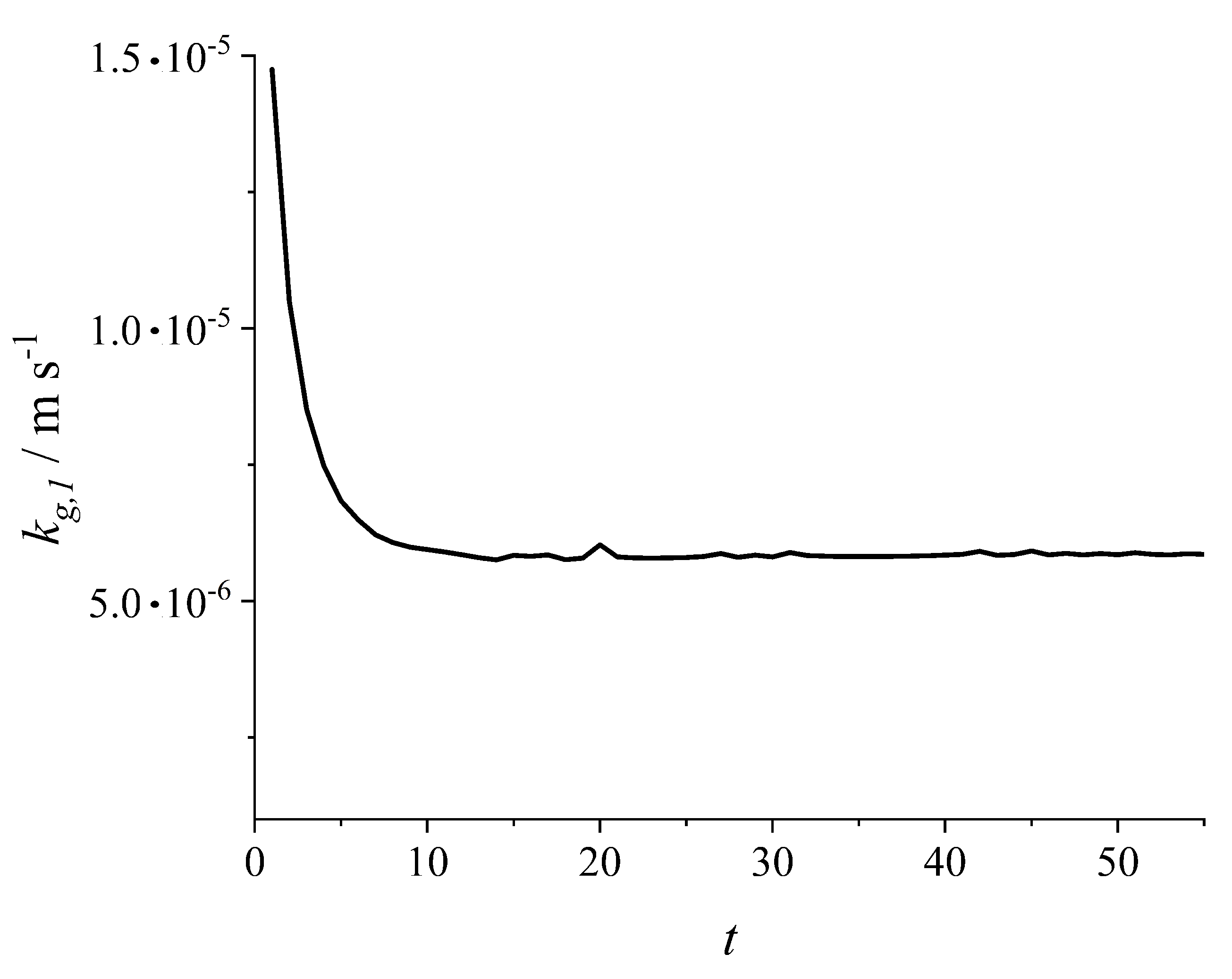
3.1. Solvate Crystallization of a Single Component

A single component crystallizing as solvate in presence of a solvent and another component will be discussed in terms of: (i) cross-diffusional effects and (ii) diffusion coefficient variations. First, the results from diffusion limited cases with and without cross-diffusion will be presented. Diffusion coefficients $D_{12}$ and $D_{21}$ were set to zero or to non-zero. Self-diffusion coefficients of the involved species were assumed to be $D_1=3\times {10}^{-10}$ m² s^$-1$, $D_2=3\times {10}^{-10}$ m² s^$-1$, and $D_3=10\times {10}^{-10}$ m² s^$-1$. These are reasonable values for ions in water, i.e., SO₄²⁻ [35]. CO₃²⁻ diffusivity was assumed to be equal. All other parameters were kept constant.

The growth coefficient to describe the integration process (compare Equation (13)) was set to $k_{r,1}=7\times {10}^{-3}$ m s^$-1$. The coefficient of phase transition is greater than diffusion resistance $D_{ii}/\Delta s$ but in the same order of magnitude. Hence, the simulated processes were mostly diffusion limited. Equilibrium molar fraction of component 1 was set to ${\tilde{x}}_1=0.0187$, which was calculated from the given mass fraction in Table 1. In Figure 3, the spatial and timely evolution in the liquid phase of all molar fractions (Diagrams (a)–(c)) and of the resulting concentrations at the point furthest away from the substrate, i.e., the impermeable (no evaporation) surface of the film (Diagram (d)) are depicted with full lines for the case that cross-diffusion is considered. Results from the same calculation but omitting cross-diffusion are depicted with dashed lines. The concentration at the point furthest away from the growing surface was chosen, because at this position, changes in diffusion behavior have the greatest impact.

Because of the moving boundary and the stationary mesh, thicknesses of the solid layer can be read from Diagrams (a)–(c). The distance between $s=0$ and the onset of concentration curves at each time step corresponds to the thickness of the solid layer at this time. The distance represents the cells $m<C$ and hence, the thickness of solid. In order to verify the calculations, the mass balances were checked.

It is evident from the diagrams that the spatial concentration profiles in the diffusion boundary layer of the liquid of all components developed immediately and independent from cross-diffusion. After three seconds, it reached nearly the end of modeling volume for all components. After five seconds process time, the concentration at $m=M$ changed noticeable. The modeling set-up predicted equilibration after about 50 s with and without consideration of cross-diffusion. Component 1 was slightly affected in its concentration development by cross-diffusion. The profiles in Diagram (a) are very similar at each time step. In Diagram (d), it can be seen that the concentration evolution at the point furthest away from the substrate with and without consideration of cross-diffusion of components 1 and 2 were alike. The concentration course of component 1 was shifted to slightly higher values whereas the enrichment of component 2 was slower and shifted to lower values without consideration of cross-diffusion. The most significant impact of considering cross-diffusion or not on concentration profiles can be observed in Diagram (b) which represents molar fraction courses of non-crystallizing component 2. Equilibration was reached earlier and the spatial profile was weaker developed with consideration of cross-diffusion than without. When considering cross-diffusion effects, the concentration at the interface increased steadily. Without considering cross-diffusion, surface concentration of component 2 reached the final steady-state value more or less immediately. Since component 1 was not affected when considering cross-diffusion, component 3 was influenced due to the closing relation ${\tilde{x}}_3=1-{\tilde{x}}_1-{\tilde{x}}_2$. As a result, simulations considering cross-diffusion predicted a stronger enrichment close to the substrate in early stages of the process. Nevertheless, the effect of considering cross-diffusion on the molar fractions is marginal. This is because of high crystallization phase transfer fluxes of the solvate. Due to that, concentration profile of component 2 became rather high and back diffusion rather strong. This resulted in a mostly independent diffusion of all components. Thus, for investigation of the influence of different diffusion coefficients, the cross-diffusion effect will be considered ($D_{ij}=D_{ji}=0$).

If a single component crystallizes, the variation of diffusion coefficients resulted in varied process times as would be expected. Higher diffusivities led to a faster development of the spatial concentration profile in the diffusion boundary layer and earlier equilibration. In Figure 4, concentration evolutions (Diagrams (a)–(c)) and concentrations at the point furthest away from the substrate (Diagram (d)) of three sets of self-diffusion coefficients are shown.

The self-diffusion coefficient of the solvent was kept constant at $D_3=10\times {10}^{-10}$ m² s^$-1$ and the others were changed in order to examine the influence of higher and lower values and significant diffusivity disagreements between component 1 and 2. The mass transfer coefficient for the integration process was set to $k_{r,1}=7\times {10}^{-3}$ m s^$-1$ and equilibrium concentration of component 1 was fixed to ${\tilde{x}}_1=0.0187$. As would be expected from independent diffusion of each material, the courses of similar diffusion coefficients of component 1 are similar - compare dashed and dotted lines. With higher diffusion coefficients, the concentrations equilibrated earlier. Also, the profile developed faster for higher diffusivities.

In case of a significant lower diffusivity of component 2 (full lines), the concentration profiles of non-crystallizing components were distorted in the diffusion boundary layer. Close to the surface in the liquid phase, component 2 enriched and a sharp concentration profile developed throughout the diffusion boundary layer. Due to the low diffusivity, material transport through diffusion was lowered, which resulted in stronger developed concentration profiles. Nevertheless, steady-state was reached after 40 s. Since component 3 (the solvent) was taken as matrix material, its concentration profiles were mostly a result from the others. After a second, molar fraction at the interface was reduced below the initial value. The point furthest away from the substrate was not affected but the course in between is characterized with a maximum molar fraction of about 0.931. Afterwards, molar fraction increased even at the furthest point. With reaching a maximum at this position, the qualitative course was similar to component 1.

When both diffusing materials have low diffusion coefficients (dotted lines), the courses are qualitatively similar for all materials but with different signs. If the diffusivities are significantly different, it results either in a drastic enrichment of the second component (full lines—$D_1/D_3=1$ and $D_2/D_3=0.3$) or of the matrix component (dashed lines—$D_1/D_3=0.3$ and $D_2/D_3=1$). This has to be taken into account for growth processes, because an enrichment of non-crystallizing material could hinder integration which was not considered in the simulations.

In Diagram (d), the molar fraction courses over time show that steady-state conditions were mostly dictated by the crystallizing component. Even though component 2 had a low diffusion coefficient in the full line case, it ran into a steady state earlier than in the dashed line case. Due to slower and ongoing crystallization of component 1, molar fraction of component 2 increased slowly at the solid-liquid interface which resulted in continuing diffusion.

By taking the concentration at the position furthest away from the substrate it is possible to retrieve overall mass transfer kinetics. By applying the power law function (Equation (22)) on the measured data, e.g., from desupersaturation measurements, it is possible to identify overall mass transfer coefficient $k_{g,i}$ and order g.

$${\dot{n}}_i=k_{g,i}·{\tilde{\rho }}^L·{({\tilde{x}}_i-{\tilde{x}}_i^{*})}^g$$

(22)

Equation (22) was applied on the data of the simulation of the single decahydrate in dotted lines ($D_1/D_3=D_2/D_3=0.3$) in Figure 4, i.e., the change of molar fraction of component 1. The mass flux ${\dot{n}}_1$ of component 1 was calculated with Equation (13). The overall mass transfer coefficient $k_{g,1}$ retrieved from the data is depicted in Figure 5 as a function of time.

The mass transfer coefficient $k_{g,1}$ takes a constant value after a short time. Prior to this point, the mass flux is mostly influenced by the varying mass transfer coefficient. Thus, after a certain process time, in this case 10 s, a constant value can be examined from desupersaturation measurements at a single point.

With the knowledge of diffusion coefficients, integration mass transfer coefficient $k_{r,i}$ in Equation (13) can be adapted such that simulation data resembles experiments. Hence, it is possible to determine concentration profiles in the diffusion boundary layer from the combination of a single point desupersaturation measurement and the presented model.

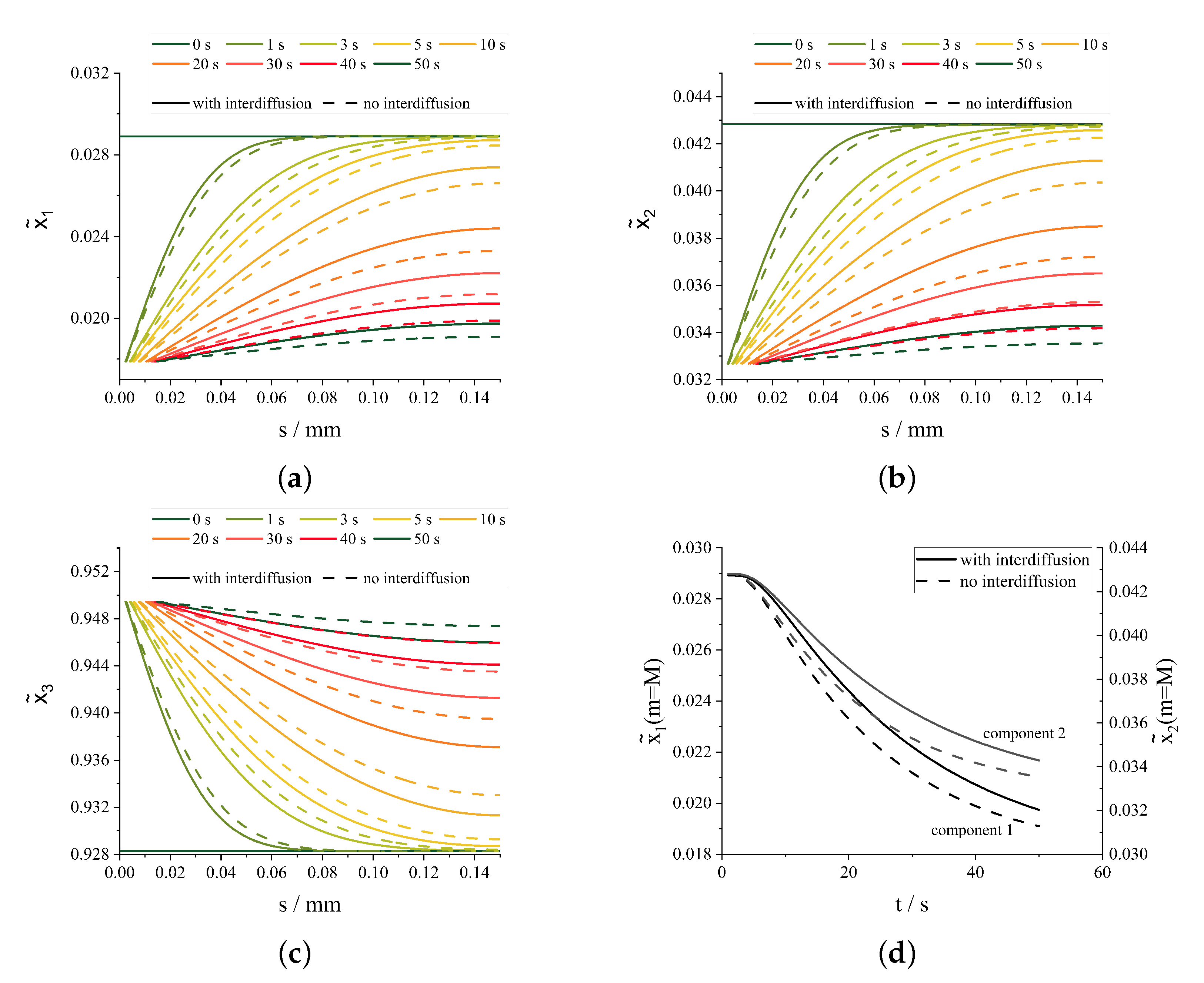
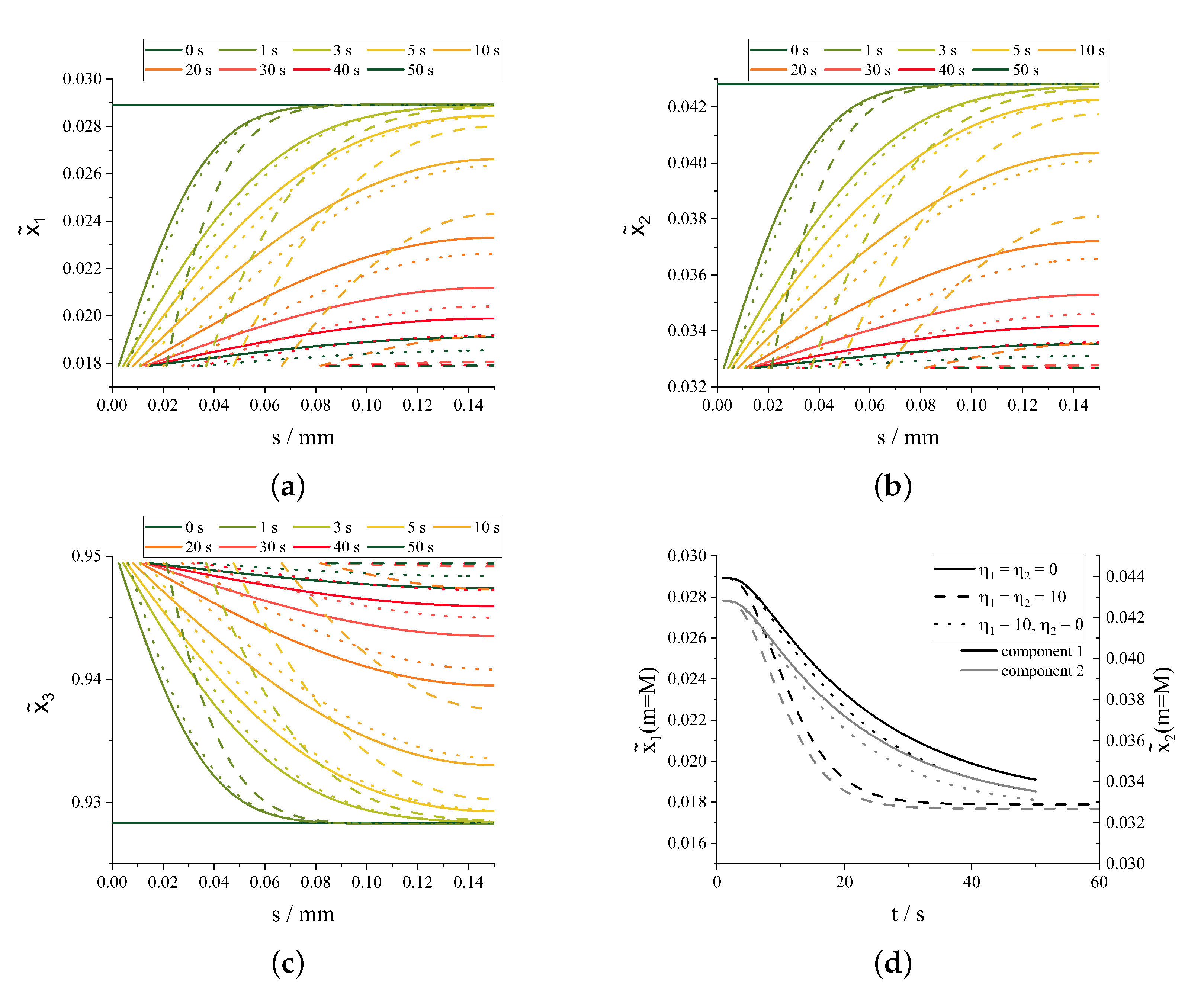
3.2. Simultaneous Crystallization of Multiple Components

First, the effect of cross-diffusion in the case simultaneous anhydrous crystallization of components 1 and 2 will be addressed (Figure 6).

Similarly to the above presented study on the effect of cross-diffusion on decahydrate crystallization (compare Figure 3), the diffusion coefficients of the three components were assumed here to be $D_1=3\times {10}^{-10}$ m² s^$-1$, $D_2=3\times {10}^{-10}$ m² s^$-1$, and $D_3=10\times {10}^{-10}$ m² s^$-1$. The Fickian diffusion coefficients were calculated according to Equations (10)–(12). The non-diagonal diffusion coefficients $D_{12}$ and $D_{21}$ of matrix $\mathbf{D}$ were either non-zero (full lines) or zero (dashed lines). The growth coefficient to describe the integration process was set to $k_{r,1}=7\times {10}^{-3}$ m s^$-1$. Equilibrium concentrations of component 1 and 2 were set to ${\tilde{x}}_1=0.0179$ and ${\tilde{x}}_2=0.0327$, respectively.

From Diagrams (a) and (b) it is visible that both diffusing components 1 and 2 are not significantly influenced by each other. Due to consideration of cross-diffusion effects, concentration profiles in the diffusion boundary layer develop a little slower compared to diffusion simulations with both components diffusing independently from each other. Hence, the time to reach equilibrium state all over the film extends. No other significant difference can be identified, which is why the consideration of interdependencies in diffusion between both dissolved materials can be disregarded. Because the solvent (component 3) concentration results from ${\tilde{x}}_3=1-{\tilde{x}}_1-{\tilde{x}}_2$, no additional observations other than those mentioned above could be made from the courses. Diagram (d) sums up the findings. The concentrations of components 1 and 2 at position $m=M$ diminished similarly. By taking into account cross-diffusion effects, the courses were shifted upward by approximately $\Delta {\tilde{x}}_i=0.001$. In case of the simultaneous crystallization of both electrolytes, the mass transport direction of both diffusing materials is the same. This influence will be neglected in the upcoming study on simultaneous crystallization of two components with different solvate states.

If two components crystallize in a three component solution there are three possible cases. First, both components crystallize as ansolvates. Second, both crystallize as solvates. Lastly, one component solidifies as a solvate the other as an ansolvate. All cases have in common that concentrations at the boundary were fixed to the equilibrium states of the two crystallizing components. The three cases are displayed in Figure 7.

All parameters disregarding the solvation number were kept constant. Self-diffusion coefficients of component 1 and 2 were equal and set to $D_i=3\times {10}^{-10}$ m² s^$-1$. Component 3 had a self-diffusion coefficient of $D_3=10\times {10}^{-10}$ m² s^$-1$. The integration mass transfer coefficients were $k_{r,i}=7\times {10}^{-3}$ m s^$-1$. Equilibrium state was set to ${\tilde{x}}_1=0.0179$ and ${\tilde{x}}_2=0.0327$ at the solid interface. In the first seconds, the concentration diffusion boundary layer developed mostly independent from solvation numbers. With lower solvation numbers—${\eta }_1={\eta }_2=0$ in full lines or ${\eta }_1=10,{\eta }_2=0$ in dotted lines—the courses are shifted left towards the solid interface in contrast to the dashed lines. This is because of the resulting solid thickness. Due to solidification of additional solvent in case three, the mass transport increased. Nevertheless, the solvation numbers had an impact on the resulting profiles later on. At the point furthest away from the substrate, concentration decreased faster and led to an earlier equilibration at higher solvation numbers. This is because of the shorter diffusion distance resulting from the moving boundary of the solid. However, equilibration of all processes took at maximum 60 s. The concentrations in Diagram (d) depict the behavior of equilibration. Just in case both components crystallized as solvates, a faster equilibration was achieved. The courses of both other cases are very similar and just slightly shifted to lower molar fraction if component 1 crystallized as a solvate. Hence, equilibration and developing profiles are strongly dependent on solvation state of crystallizing materials or on the mass transfer to the solid, respectively.

4. Discussion

Multi-component diffusion in the liquid phase during mostly diffusion limited crystallization processes were modeled using the Fickian approach. Influences of diffusivities or solvation states of the different materials on concentration profiles in the diffusion boundary layer were studied. Self-diffusion coefficients were varied to show their impact on the developement of concentrations in the diffusion boundary layer ($3\times {10}^{-10}$ m² s^$-1$$\le D_i\le {10}^{-9}$ m² s⁻¹). With significantly different diffusion coefficients, the enrichment of solvent or of other non-crystallizing materials at the interface was predicted. The change in concentration at the integration interface will have an impact on co-crystal growth. If the available amount of co-crystallizing components deviates from the stoichiometrically desired values, other solids are stable with respect to phase equilibria and crystallize at the surface.

The importance of considering cross-diffusion effects was investigated in case of crystallization of a single decahydrate and simultaneous crystallization of two anhydrates. It was found to be not significantly relevant on the resulting concentration profiles in the diffusion boundary layer. The neglection of cross-diffusion effects was attributed to the fact that phase transfer fluxes of solvates were rather high, which resulted in a strong development of concentration profiles in the diffusion boundary layer. Hence, the diffusion driving force of both components was rather strong, which is why cross-diffusion effects play a minor role. In case of the simultaneous crystallization of both electrolytes, the mass transport direction of both diffusing materials is the same. Hence, interdependencies between both components during diffusion diminished. However, it is imaginable that cross-diffusion effects have to be considered in cases of crystallization of single hydrates with fewer water atoms. Additionally, the influence of the effect has to be examined experimentally.

Integration limited processes were not part of the investigation. Nevertheless, it would be easy to incorporate integration limitation by reducing mass transfer coefficient $k_{r,i}$ in Equation (13) and hence, in simulation.

In addition to simulative studies, the presented model offers the opportunity to extract kinetic parameters from experimental data and to obtain not measurable concentration profiles in the diffusion boundary layer. With the knowledge of diffusion coefficients, it is solely necessary to measure the concentration at a single point in solution experimentally and adapt the kinetic coefficient $k_{r,i}$ in the model such that timely concentration trends at the specific single point equal the calculated concentration trends of the model at the same position. As was shown with concentration courses at position $m=M$ in diagrams (d) of Figure 3, Figure 4, Figure 5, Figure 6 and Figure 7, desupersaturation measurements at a single point are performable in reasonable time-scales even for diffusion limited growth processes, which represent the fastest possible growth process. Hence, it is possible to retrieve the two unknown variables $k_{g,i}$ and g in mass transfer kinetic equations, e.g., Equation (22), from desupersaturation measurements.

Desupersaturation measurements relating to this theoretical study were conducted recently by Helfenritter and Kind [41].

References

1. Guignon, B.; Duquenoy, A.; Dumoulin, E.D. Fluid bed encapsulation of particles: Principles and practice. Dry. Technol. 2002, 20, 419–447. [Google Scholar] [CrossRef]
2. Degrève, J.; Baeyens, J.; van de Velden, M.; de Laet, S. Spray-agglomeration of NPK-fertilizer in a rotating drum granulator. Powder Technol. 2006, 163, 188–195. [Google Scholar] [CrossRef]
3. Suresh, P.; Sreedhar, I.; Vaidhiswaran, R.; Venugopal, A. A comprehensive review on process and engineering aspects of pharmaceutical wet granulation. Chem. Eng. J. 2017, 328, 785–815. [Google Scholar] [CrossRef]
4. Römbach, E.; Ulrich, J. Self-controlled coating process for drugs. Cryst. Growth Des. 2007, 7, 1618–1622. [Google Scholar] [CrossRef]
5. Shin, G.S.; Choi, W.G.; Na, S.; Ryu, S.O.; Moon, T. Rapid crystallization in ambient air for planar heterojunction perovskite solar cells. Electron. Mater. Lett. 2017, 13, 72–76. [Google Scholar] [CrossRef]
6. Sakai, N.; Pathak, S.; Chen, H.W.; Haghighirad, A.A.; Stranks, S.D.; Miyasaka, T.; Snaith, H.J. The mechanism of toluene-assisted crystallization of organic–inorganic perovskites for highly efficient solar cells. J. Mater. Chem. A 2016, 4, 4464–4471. [Google Scholar] [CrossRef]
7. Nijdam, J.; Trouillet, V.; Kachel, S.; Scharfer, P.; Schabel, W.; Kind, M. Coat formation of surface-active proteins on aqueous surfaces during drying. Colloids Surf. B Biointerfaces 2014, 123, 53–60. [Google Scholar] [CrossRef]
8. Seo, K.S.; Han, H.K. Multilayer-coated tablet of clopidogrel and rosuvastatin: Preparation and in vitro/in vivo characterization. Pharmaceutics 2019, 11, 313. [Google Scholar] [CrossRef] [Green Version]
9. Song, K.S.; Lim, J.; Yun, S.; Kim, D.; Kim, Y. Composite fouling characteristics of CaCO3 and CaSO4 in plate heat exchangers at various operating and geometric conditions. Int. J. Heat Mass Transf. 2019, 136, 555–562. [Google Scholar] [CrossRef]
10. Lv, Y.; Lu, K.; Ren, Y. Composite crystallization fouling characteristics of normal solubility salt in double-pipe heat exchanger. Int. J. Heat Mass Transf. 2020, 156, 119883. [Google Scholar] [CrossRef]
11. Yuan, J.J.; Stepanski, M.; Ulrich, J. Fremdstoffeinflüsse auf Kristallwachstumsgeschwindigkeiten bei der Kristallisation aus Lösungen. Chem. Ing. Tech. 1990, 62, 645–646. [Google Scholar] [CrossRef]
12. Rauls, M.; Bartosch, K.; Kind, M.; Lacmann, R.; Mersmann, A. The influence of impurities on crystallization kinetics–a case study on ammonium sulfate. J. Cryst. Growth 2000, 213, 116–128. [Google Scholar] [CrossRef]
13. Vergara, A.; Paduano, L.; Vitagliano, V.; Sartorio, R. Multicomponent diffusion in solutions where crystals grow. Mater. Chem. Phys. 2000, 66, 126–131. [Google Scholar] [CrossRef]
14. Kubota, N. Effect of impurities on the growth kinetics of crystals. Cryst. Res. Technol. J. Exp. Ind. Crystallogr. 2001, 36, 749–769. [Google Scholar] [CrossRef]
15. Louhi-Kultanen, M.; Kallas, J.; Partanen, J.; Sha, Z.; Oinas, P.; Palosaari, S. The influence of multicomponent diffusion on crystal growth in electrolyte solutions. Chem. Eng. Sci. 2001, 56, 3505–3515. [Google Scholar] [CrossRef]
16. Zago, G.P.; Penha, F.M.; Seckler, M.M. Product characteristics in simultaneous crystallization of NaCl and CaSO4 from aqueous solution with seeding. Desalination 2020, 474, 114180. [Google Scholar] [CrossRef]
17. Penha, F.M.; Andrade, F.R.D.; Lanzotti, A.S.; Moreira Junior, P.F.; Zago, G.P.; Seckler, M.M. In Situ Observation of Epitaxial Growth during Evaporative Simultaneous Crystallization from Aqueous Electrolytes in Droplets. Crystals 2021, 11, 1122. [Google Scholar] [CrossRef]
18. Chiarella, R.A.; Davey, R.J.; Peterson, M.L. Making co-crystals the utility of ternary phase diagrams. Cryst. Growth Des. 2007, 7, 1223–1226. [Google Scholar] [CrossRef]
19. Urbanus, J.; Roelands, C.M.; Verdoes, D.; Jansens, P.J.; ter Horst, J.H. Co-crystallization as a separation technology: Controlling product concentrations by co-crystals. Cryst. Growth Des. 2010, 10, 1171–1179. [Google Scholar] [CrossRef]
20. Mersmann, A. Crystallization Technology Handbook; CRC Press: Boca Raton, FL, USA, 2001. [Google Scholar]
21. Sun, C.C. Cocrystallization for successful drug delivery. Expert Opin. Drug Deliv. 2013, 10, 201–213. [Google Scholar] [CrossRef]
22. Pawar, N.; Saha, A.; Nandan, N.; Parambil, J.V. Solution cocrystallization: A scalable approach for cocrystal production. Crystals 2021, 11, 303. [Google Scholar] [CrossRef]
23. Burton, J.A.; Prim, R.C.; Slichter, W.P. The distribution of solute in crystals grown from the melt. Part I. Theoretical. J. Chem. Phys. 1953, 21, 1987–1991. [Google Scholar] [CrossRef]
24. Garside, J.; Mersmann, A.; Nývlt, J. Measurement of Crystal Growth and Nucleation Rates; IChemE: Rugby, UK, 2002. [Google Scholar]
25. Eder, C.; Choscz, C.; Müller, V.; Briesen, H. Jamin-interferometer-setup for the determination of concentration and temperature dependent face-specific crystal growth rates from a single experiment. J. Cryst. Growth 2015, 426, 255–264. [Google Scholar] [CrossRef]
26. Lin, H.; Rosenberger, F.; Alexander, J.I.; Nadarajah, A. Convective-diffusive transport in protein crystal growth. J. Cryst. Growth 1995, 151, 153–162. [Google Scholar] [CrossRef]
27. Gupta, A.; Shim, S.; Issah, L.; McKenzie, C.; Stone, H.A. Diffusion of multiple electrolytes cannot be treated independently: Model predictions with experimental validation. Soft Matter 2019, 15, 9965–9973. [Google Scholar] [CrossRef]
28. Caspari, W.A. CCCXXIV.—The system sodium carbonate–sodium sulphate–water. J. Chem. Soc. Trans. 1924, 125, 2381–2387. [Google Scholar] [CrossRef]
29. von Plessen, H. Sodium Sulfates. In Ullmann’s Encyclopedia of Industrial Chemistry; John Wiley & Sons, Ltd.: Hoboken, NJ, USA, 2000. [Google Scholar] [CrossRef]
30. Thieme, C. Sodium Carbonates. In Ullmann’s Encyclopedia of Industrial Chemistry; John Wiley & Sons, Ltd.: Hoboken, NJ, USA, 2000. [Google Scholar] [CrossRef]
31. Taylor, R.; Krishna, R. Multicomponent Mass Transfer; John Wiley & Sons, Ltd.: Hoboken, NJ, USA, 1993; Volume 2. [Google Scholar]
32. Rehfeldt, S.; Stichlmair, J. Measurement and calculation of multicomponent diffusion coefficients in liquids. Fluid Phase Equilibria 2007, 256, 99–104. [Google Scholar] [CrossRef]
33. Krishna, R.; van Baten, J.M. The darken relation for multicomponent diffusion in liquid mixtures of linear alkanes: An investigation using molecular dynamics (MD) simulations. Ind. Eng. Chem. Res. 2005, 44, 6939–6947. [Google Scholar] [CrossRef]
34. Kim, S.U.; Srinivasan, V. A Method for Estimating Transport Properties of Concentrated Electrolytes from Self-Diffusion Data. J. Electrochem. Soc. 2016, 163, A2977. [Google Scholar] [CrossRef]
35. Nielsen, J.M.; Adamson, A.W.; Cobble, J.W. The self-diffusion coefficients of the ions in aqueous sodium chloride and sodium sulfate at 25. J. Am. Chem. Soc. 1952, 74, 446–451. [Google Scholar] [CrossRef]
36. Liu, X.; Schnell, S.K.; Simon, J.M.; Krüger, P.; Bedeaux, D.; Kjelstrup, S.; Bardow, A.; Vlugt, T.J.H. Diffusion coefficients from molecular dynamics simulations in binary and ternary mixtures. Int. J. Thermophys. 2013, 34, 1169–1196. [Google Scholar] [CrossRef]
37. Stejskal, E.O.; Tanner, J.E. Spin diffusion measurements: Spin echoes in the presence of a time–dependent field gradient. J. Chem. Phys. 1965, 42, 288–292. [Google Scholar] [CrossRef] [Green Version]
38. Parkhurst, D.L.; Appelo, C.A.J. Description of Input and Examples for PHREEQC Version 3: A Computer Program for Speciation, Batch-Reaction, One-Dimensional Transport, and Inverse Geochemical Calculations; U.S. Geological Survey: Denver, CO, USA, 2013.
39. Marion, G.M.; Mironenko, M.V.; Roberts, M.W. FREZCHEM: A geochemical model for cold aqueous solutions. Comput. Geosci. 2010, 36, 10–15. [Google Scholar]
40. Hirt, C.W.; Nichols, B.D. Volume of fluid (VOF) method for the dynamics of free boundaries. J. Comput. Phys. 1981, 39, 201–225. [Google Scholar] [CrossRef]
41. Helfenritter, C.; Kind, M. Determination of crystal growth rates in multi-component solutions. Cryst. Growth Des. 2022. in review process. [Google Scholar]
Figure 1. Diagram (a) represents concentration evolution in a slab of a solution of two components dissolved in a solvent. The special case of only one component (component 2) crystallizing while both other components do not crystallize is shown. The two non-crystallizing components level-up in the liquid phase. In Diagram (b), simultaneous crystallization of components 1 and 2 is depicted. Again, at the solid-liquid interface concentrations are set to equilibrium. Here, only the solvent enriches in the vicinity of the interface.
Crystals 12 00872 g001
Figure 2. The numerical model: At m = C concentrations of crystallizing component are set to equilibrium conditions. No flux condition prevails for non-crystallizing components. At m = M , no flux condition for all components applies. The cells in between are modeled by Equation (9).
Crystals 12 00872 g002
Figure 3. Time and space evolution of molar fractions of component 1 (a), 2 (b), and 3 (c). Diagram (d) shows the development of the molar fraction x ˜ i of the dissolved components at the point m = M . Data with consideration of cross-diffusion is represented by full lines whereas the dashed lines illustrate the same case, but without cross-diffusion.
Crystals 12 00872 g003
Figure 4. Simulated evolution in time and space of molar fractions of component 1 (a), 2 (b), and 3 (c) in solution. Diagram (d) shows the development of the molar fraction x ˜ i ( i = 1 , 2 ) at m = M . Full lines represent the results with self-diffusion coefficients of: D 1 / D 3 = 1 and D 2 / D 3 = 0.3 . Dashed lines show the results of reduced diffusion coefficient of component 1 ( D 1 / D 3 = 0.3 and D 2 / D 3 = 1 ). Finally, dotted lines stand for reduced coefficients of both materials ( D 1 / D 3 = D 2 / D 3 = 0.3 ).
Crystals 12 00872 g004
Figure 5. Time dependent overall mass transfer coefficient k g , 1 retrieved from the simulative study in Figure 5 with diffusion coefficient ratios of D 1 / D 3 = D 2 / D 3 = 0.3 (dotted lines).
Crystals 12 00872 g005
Figure 6. Time and space evolution of molar fractions of component 1 (a), 2 (b), and 3 (c) in solution. Diagram (d) depicts the development of the concentration x ˜ i at the point m = M over time. Simultaneous crystallization of component 1 and 2 are shown with and without consideration of cross-diffusion effects. Full lines represent cases with consideration of cross-diffusion. Dashed lines show results of simulation without consideration of cross-diffusion.
Crystals 12 00872 g006
Figure 7. Time and space evolution of molar fractions of component 1 (a), 2 (b), and 3 (c) in solution. Diagram (d) depicts the development of the concentration x ˜ i at the point m = M over time. Simultaneous crystallization of component 1 and 2 are shown with different solvation states of either material. Full lines represent cases with no solvation building ( η 1 = η 2 = 0 ). Dashed lines represent the result if both components solidify as decasolvates ( η 1 = η 2 = 10 ). The crystallization of a solvate and an ansolvate is given by dotted lines ( η 1 = 10 , η 2 = 0 ).
Crystals 12 00872 g007