Anharmonic Motion in the Crystal Structure of 2-Mercaptopyridone

Abstract

With the present study, we revise earlier results about the title compound 2-mercaptopyridone in which the deformation density was determined from an X–N study in 1982 (X-ray, neutron diffraction). In the current X–X study (X-ray, X-ray), anharmonic motion parameters for the atoms were included and it resulted in a very clean deformation density map without the unexplainable features of the literature results. The presence of anharmonic effects is supported by a study of the thermal expansion in the temperature range 100–260 K. A topological study of the electron density confirms a bond length alternation in the six-membered ring. The calculation of the electrostatic potential indicates that the N–H⋯S hydrogen bond is an electrostatic interaction, and that other attractive intermolecular contacts are probably dispersive.

1. Introduction

2-Mercaptopyridone (I) occurs in two tautomeric forms (Scheme 1) which are in equilibrium with each other. In the gas phase, the thiolpyridine form is the more stable tautomer [1]. In solution, the equilibrium depends on the solvent polarity [2]. In the crystal structure, only the thiopyridone form exists. This was elucidated by Penfold in 1953 based on photographic methods and two-dimensional electron density projections [3]. Later, it was confirmed by more detailed three-dimensional studies at room temperature [4] and at T = 116 K [5].

The room temperature analysis by Ohms et al. contains X-ray and neutron data, and a comparison between the two [4]. The X–N map gives an impression of the deformation density but it shows unexplainable features in the proximity of the sulfur atom. The authors ascribe this to a difference in the anisotropic displacement parameters between the X-ray and the neutron results. In order to obtain more insight into the situation of the sulfur atom, we performed a high-resolution X-ray study and applied different atomic models in the structure refinement.

An intrinsic challenge of X-ray diffraction studies is that the distribution of the electron density is convoluted with the effects of thermal motion. For the evaluation of the deformation density and other quantum chemical properties, the separation of non-spherical electron density and thermal motion becomes essential. The success of this separation needs to be checked by testing the physical plausibility of the electron density as well as the thermal motion. Many cases in the literature show that the thermal motion can be described by a harmonic model, the classical thermal ellipsoids. In other cases, it appeared to be necessary to include a model with anharmonic motion parameters. This often concerns heavy-atom compounds but examples of purely organic compounds are also well known (e.g., [6,7]).

2. Materials and Methods

2-Mercaptopyridone was purchased from Sigma-Aldrich, Amsterdam, Netherlands and re-crystallized by slow evaporation of a solution in acetone. The crystals tend to agglomerate.

For the high-resolution experiment and for the temperature-dependent study, two different crystals were used. All measurements were performed on a Bruker Kappa ApexII diffractometer (Karlsruhe, Germany) with sealed tube, Triumph monochromator, and $Mo-K_{\alpha }$ radiation ($\lambda =0.71073$ Å). Intensity integration and the refinement of diffractometer geometries and orientation matrices were performed with programs from the Eval15 suite [8]. An isotropic mosaicity of 0.35${}^{\circ }$ (high-resolution study) and 0.50${}^{\circ }$ (temperature-dependent study) was assumed for the prediction of reflection profiles in Eval15. The SADABS program [9] was used for absorption correction and scaling. In SADABS, the following error model was applied for the individual, unmerged reflections: ${\sigma }_{new}^2={[K\times {\sigma }_{Eval15}]}^2+{[g\times 〈I〉]}^2$, where $g=0.0242$ and $K=0.836-1.562$. The final $\sigma$-values for the least-squares refinement were obtained by merging the individual reflections. All statistical tests in the current study are based on these merged $\sigma$-values, i.e., before applying a weighting scheme.

The temperature-dependent study was performed by ${360}^{\circ }\varphi$ rotations with an increment of 0.3${}^{\circ }$. The detector was kept fixed at a distance of 40 mm and a swing angle of $2\theta ={20}^{\circ }$. The exposure time was 10 s per image. In the structure refinements of the temperature-dependent data, non-hydrogen atoms were refined freely with anisotropic displacement parameters and the N–H hydrogen atoms with isotropic displacement parameters. C–H hydrogen atoms were refined with a riding model.

For the high-resolution experiment, a total of 47 $\varphi$ and $\omega$ scans was performed. One fast scan was performed with a rotation increment of 0.3${}^{\circ }$ and a generator setting of 50 kV, 8 mA. The other 46 scans were performed with a rotation increment of $0.5^{\circ }$ and a generator setting of 50 kV, 30 mA. Overall, this resulted in 12,853 images. The exposure time was selected as 1, 2, 10 or 30 s. Further details about the refinement results are given in

Table 1. Experimental details.

High-Resolution Refinements of (I)
sum formula	${\mathrm{C}}_5{\mathrm{H}}_5\mathrm{NS}$
formula weight	111.16
crystal system	monoclinic
space group	$P{2}_1/c$
a	6.02927(6) Å
b	6.26010(6) Å
c	14.10858(13) Å
$\beta$	101.808(1) ${}^{\circ }$
V	521.243(9) Å${}^3$
Z	4
$D_x$	1.416 $\mathrm{g}/{\mathrm{cm}}^3$
$\mu$	0.47 ${\mathrm{mm}}^{-1}$
T	100(2) K
crystal size	$0.43\times 0.37\times 0.24$ mm
${(sin\theta /\lambda )}_{max}$	1.24 Å${}^{-1}$
absorption corr.	multi-scan (SADABS [9])
corr. range	0.85–0.93
meas. refl.	114,524
unique refl.	8374
$R_{int}$	0.022
	IAM	NoSpherA2	Multipole
reflection merging	SHELXL [12]	Olex2 [13]	XPREP [14]
refinement program	SHELXL [12]	Olex2 [13]	XD [15]
refinement on	$F^2$	$F^2$	F
used refl.	8374	8374	8115
no. parameters	84	109	377
no. restraints	0	0	0
weight_a, weight_b	0.0486, 0.0072	0.0130, 0.0049	0.0102, 0.0020
R (all ref.)	0.0228	0.0146	0.014
wR (all refl.)	0.0775	0.0292	0.011
S	1.109	1.0097	1.036
$\Delta {\rho }_{min/max}$ [e/Å${}^3$]	−0.26/0.57	−0.27/0.28	−0.15/0.09

. The non-spherical scattering factors for NoSpherA2 [10] were derived from iterative calculations with the pySCF software [11] using the B3LYP method, a def2-TZVPPD basis set and the hydrogen-bonded dimer as input. For the final XD refinement, the $\sigma$-values in the reflection file were adapted according to a SHELXL-type weighting scheme resulting in a goodness of fit close to 1.

3. Results and Discussion

3.1. Independent Atom Model

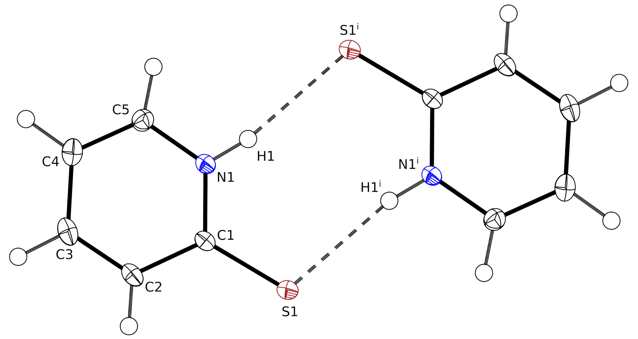
Structure refinement with spherical scattering factors from an independent atom model was performed with the SHELXL software [12]. Selected bond lengths are given in

Table 2. Intramolecular geometry in (I) after refinement with the independent atom model. In square brackets, the room-temperature X-ray results of [4] are given for comparison.

Bond Distances [Å]		Bond Angles [${}^{\circ }$]
N1–C5	1.3552(3) [1.354(3)]	N1–C5–C4	120.68(2) [120.7(2)]
N1–C1	1.3623(2) [1.357(3)]	C5–N1–C1	124.531(16) [124.6(2)]
C1–C2	1.4201(2) [1.417(4)]	N1–C1–C2	115.572(17) [115.0(2)]
C2–C3	1.3779(3) [1.376(4)]	C3–C2–C1	120.88(2) [120.9(2)]
C3–C4	1.4104(4) [1.399(4)]	C2–C3–C4	120.685(18) [120.6(3)]
C4–C5	1.3689(3) [1.352(4)]	C5–C4–C3	117.63(2) [118.0(3)]
S1–C1	1.69981(19) [1.692(2)]	N1–C1–S1	120.368(12) [120.6(2)]
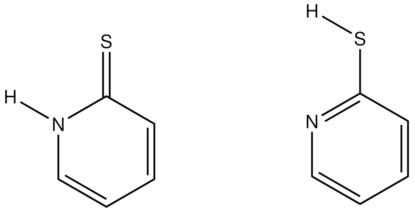
		C2–C1–S1	124.052(15) [124.3(2)]

. The C–C bond lengths show a significant alternation. Bonds C2–C3 and C4–C5 are significantly shorter than C1–C2 and C3–C4. The C–S bond of 1.69981(19) Å confirms the double-bond character. All hydrogen atoms were located in difference Fourier maps and refined freely with isotropic displacement parameters. They clearly show the protonation of the nitrogen atom. Overall, this is consistent with the expectation for the thiopyridone form (Scheme 1) and with the quantum-theoretical geometry of it, as calculated in 2002 in vacuo [1]. A comparison with the room-temperature X-ray results of [4] shows mainly the increased precision of the current data (Table 2).

In the crystal, the molecules form centrosymmetric hydrogen-bonded dimers with the N–H group as donor and the sulfur as acceptor (Figure 1). The graph set for this dimer is $R_2^2\left(8\right)$. The corresponding inversion center is located at $(0,\frac{1}{2},0)$, Wyckoff position c.

The inversion at $(0,0,0)$, Wyckoff position a, generates an antiparallel molecule with a perpendicular distance of 3.3949(1) Å. Based on the literature [16], we consider such a short distance as an indication for a $\pi \cdots \pi$ stacking interaction. In this arrangement, the ring centers are not located exactly on top of each other. The distance between the ring centers is 3.6714(2) Å, resulting in a ring slippage of 1.40 Å.

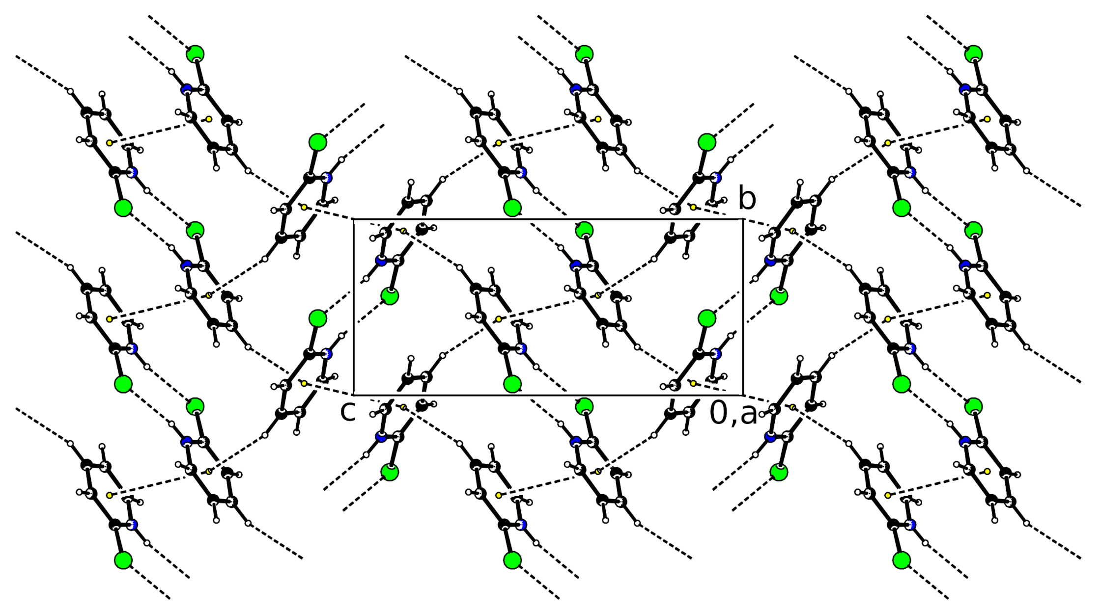
While the $\pi \cdots \pi$ stacking interaction concerns one side of the molecule, the opposite side is involved as acceptor of a C–H$\cdots \pi$ interaction. C–H$\cdots \pi$ interactions mainly have a dispersive nature. Despite their weakness, they can be influential [17] as well as in small-molecule structures [18] as in proteins [19]. An overall impression of the intermolecular interactions in (I) is depicted in Figure 2. The weak interactions result in a layer formation in the $b,c$ plane.

Symmetry considerations lead to the conclusion that the molecule is located in a general position without symmetry but the planarity of the molecule gives rise to an approximate mirror symmetry ($C_s$ symmetry) with an r.m.s. deviation from ideal symmetry of only 0.017 Å. The formation of the hydrogen-bonded $R_2^2\left(8\right)$ dimer disturbs this approximate symmetry only slightly. The r.m.s. deviation from ideal $C_{2h}$ symmetry of the dimer is only 0.063 Å. The crystal field for the molecule, however, is non-symmetric, with $\pi \cdots \pi$ stacking on one side, and a C–H$\cdots \pi$ interaction on the other side.

So far, the discussion of intermolecular interactions in (I) has been based on pure geometrical calculations performed with the PLATON software [20]. An alternative approach is the calculation and analysis of the Hirshfeld surface which is based on electron densities [21]. The ratio between the electron density of the promolecule and the electron density of the procrystal is calculated, and an isosurface is drawn where this ratio is 0.5. 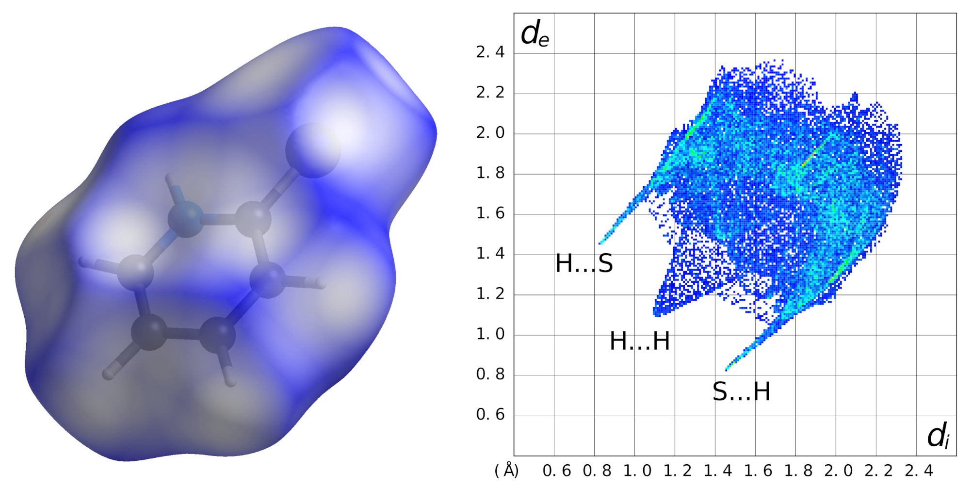It is a straightforward way to recognize all kinds of intermolecular interactions: the value of $d_{norm}$ becomes negative if the intermolecular distance is shorter than the van der Waals separation. For (I), the Hirshfeld surface is shown in Figure 3 (left). Hydrogen atoms occupy 63.1%, carbon 15.3%, nitrogen 2.8% and sulfur 18.8% of this surface. In the fingerprint plot (Figure 3, right), H⋯S/S⋯H and H⋯H contacts are most prominent.

Following a procedure by Jelsch et al. [22], it is possible to use the fingerprint plot (Figure 3) to calculate an enrichment ratio E for each intermolecular contact. Enrichment ratios larger than unity indicate contacts which are preferred in the crystal packing. The system tries to avoid contacts with $E<1$. For (I), the enrichment ratios are given in

Table 3. Enrichment ratios E calculated from the fingerprint plot in Figure 3 using the algorithm of [22]. Values larger than unity are printed in bold. Entries where no reliable value could be obtained are marked with /.

	H	C	N	S
H	0.85
C	1.09	1.46
N	0.84	/	/
S	1.47	0.09	0.0	0.31

. The H⋯S/H⋯S and C⋯C contacts appear to be important for the packing which corresponds to the N–H⋯S hydrogen bonds and the $\pi \cdots \pi$ stacking (discussed above). The enrichment ratio for the H⋯C contacts is only slightly above 1. The positive influence of the C–H$\cdots \pi$ interactions might thus be small. From this analysis, H⋯H contacts are unfavorable. In this context, we note that the shortest intermolecular H⋯H contact is between H5 and H5${}^i$ ($i:-x-1,-y,-z$) with 2.345(10) Å (SHELXL results) or 2.18 Å (normalized C–H distances). This is smaller than the van der Waals distance of 2.40 Å.

For an analysis of the anisotropic displacement parameters, the result of the current refinement was subjected to a rigid-body TLS analysis using the THMA11 software [23]. The weighted R value for the TLS model is 0.028. ($R={[\sum {(w{U}_{obs}-w{U}_{calc})}^2/\sum {\left(w{U}_{obs}\right)}^2]}^{1/2}$ with $w=\langle \sigma \rangle /\sigma$). This low R value is a clear sign that the observed atomic displacement parameters can be well fitted with a rigid-body TLS model.

The THMA11 program additionally performs a MSDA analysis (“Hirshfeld rigid-bond test” [24]). The MSDA ${\Delta }_{A,B}$ for the S1–C1 bond is 0.0008 Å${}^2$, a value larger than expected. If this situation is related to the problems of this bond in the X–N analysis by Ohms et al. [4] (vide supra) cannot be decided on the independent atom model.

3.2. Thermal Expansion

A temperature-dependent diffraction experiment was performed to obtain better insight into the thermal behavior of (I). In order to improve the internal consistency, the movable detector was kept at a fixed position for the duration of the experiment. The resulting unit cell parameters are provided in Table S1 (Supplementary Materials). It appears that the largest expansion with temperature is along the c axis, and the smallest along the b axis (see Figure S1, Supplementary Materials).

A more appropriate analysis of the temperature dependence of the unit cell is the calculation of the anisotropic thermal expansion tensor. This is a symmetric second-rank tensor [25]. In the monoclinic case, the tensor has four independent values. For the calculation, we used the STRAIN ANALYSIS routine of the PLATON software [20] which uses the algorithm of Ohashi [26]. According to the convention, the result is expressed in Cartesian space. (Definition for the current orthogonalization: $x\Vert a,z\Vert c^{★},y\Vert (z\times x)$.) Based on the unit cell parameters at 100 and 260 K, we obtain the following unit strain tensor ($\times {10}^6$ K${}^{-1}$):

$$\left(\begin{array}{ccc}62.3912& 0.0000& -57.7812\\ 0.0000& 47.2099& 0.0000\\ -57.7812& 0.0000& 66.0993\end{array}\right)$$

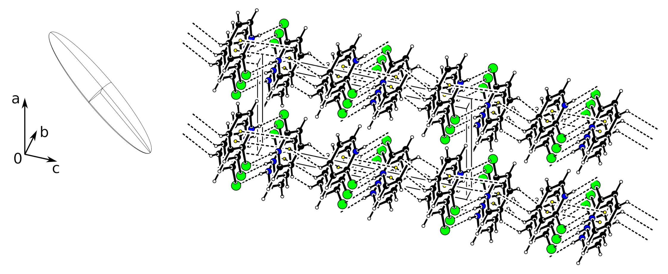
The corresponding eigenvalues are 122.1(6), 47.2(7) and 6.4(6) ($\times {10}^6$). Consequently, the representation of the tensor as an ellipsoid shows the large anisotropy (Figure 4). The directions of the largest and the smallest expansion are both in the $a,c$ plane. The largest expansion direction forms an angle of $32.3{\left(2\right)}^{\circ }$ with the c axis, and $134.1{\left(2\right)}^{\circ }$ with the a axis. This direction coincides approximately with the direction of the C–H$\cdots \pi$ interaction (vide supra).

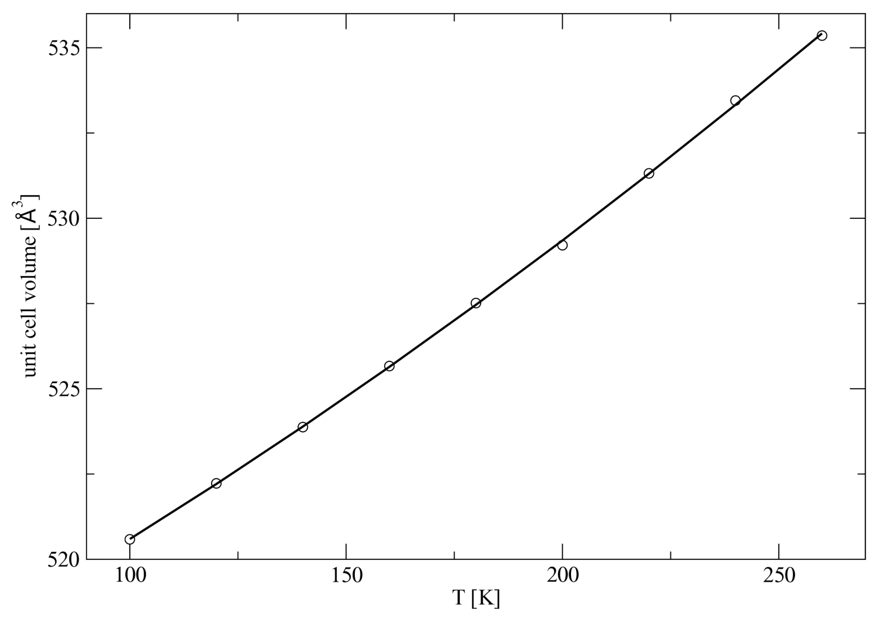
It should be noted that the expansion of the unit cell parameters (Figure S1) cannot be properly fitted by a linear regression. Quadratic functions had to be used instead. Similarly, the volume expansion also needs a quadratic fit (Figure 5).

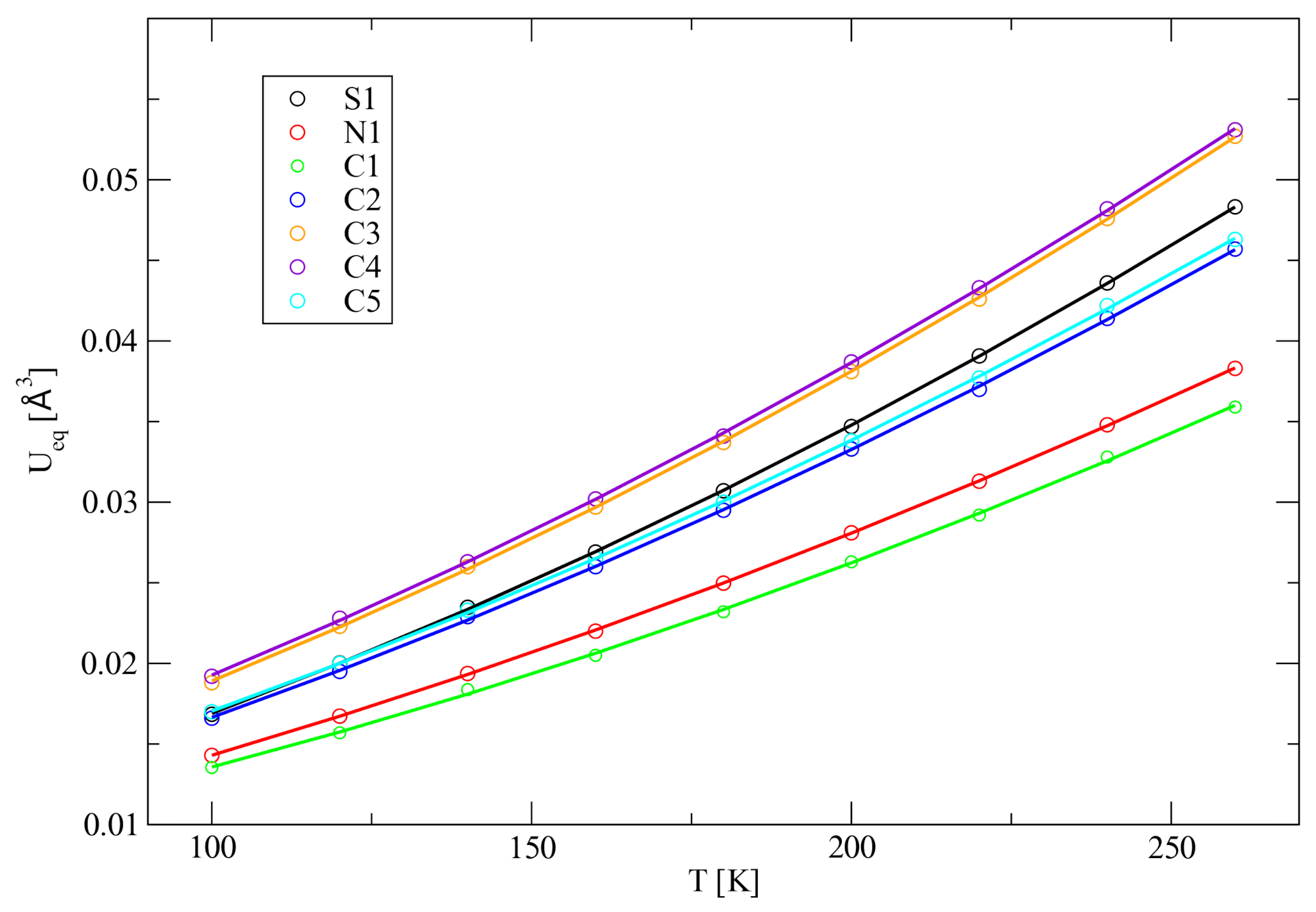
The measurements at nine different temperatures by single ${360}^{\circ }\varphi$ scans not only allowed the determination of unit cell parameters but were also sufficient for structure refinements. Data completeness was 99.9–100.0% at $\theta =25.{24}^{\circ }$ and 87.6–89.5% at the maximum resolution of $\theta$ = 30.58–30.73${}^{\circ }$. From the refinement results, it becomes clear that the atomic displacement parameters do not increase linearly with temperature but a quadratic regression is needed to fit the data points (Figure 6). Such non-linear behaviour can be associated with anharmonicity [27]. A quadratic fit is also necessary to fit the temperature dependence of the eigenvalues of the T- and L-tensors, respectively, if the anisotropic displacement parameters are subjected to a TLS rigid-body fit (Figures S2 and S3).

Table 4. Geometries of C–H$\cdots \pi$ interactions in (I). $Cg$: center of gravity of six-membered ring. Symmetry code $i:-x,y-\frac{1}{2},\frac{1}{2}-z$. H-Perp is the perpendicular distance of the hydrogen atom H3 from the ring plane.

T [K]	H3⋯Cg${}^{\mathit{i}}$ [Å]	H-Perp [Å]	C3-H3⋯Cg${}^{\mathit{i}}$ [${}^{\circ }$]	C3⋯Cg${}^{\mathit{i}}$ [Å]
100	2.76	2.74	134	3.4893(12)
120	2.77	2.75	134	3.4984(12)
140	2.78	2.76	134	3.5079(12)
160	2.79	2.77	134	3.5177(12)
180	2.80	2.78	134	3.5275(13)
200	2.81	2.79	134	3.5373(14)
220	2.83	2.81	134	3.5489(15)
240	2.85	2.82	134	3.5602(16)
260	2.86	2.84	134	3.5715(16)

presents the temperature dependence of the intermolecular C–H$\cdots \pi$ interaction. We see an increase of 0.082(2) Å for the C3⋯Cg distance over the observed temperature range. This is larger than the increase in the $\pi \cdots \pi$ stacking interaction (0.0635(6) Å, Table S3) and significantly larger than the increase in the N–H⋯S hydrogen bond (0.0090(14) Å, Table S2). This observation is consistent with the shape and orientation of the thermal expansion tensor. We see here another example for the fact that the thermal expansion tensor is related to the strength of intermolecular bonds [28]. The stronger the intermolecular bond, the smaller is the expansion.

3.3. Hirshfeld Atom Refinement

Analysis of the difference electron density of the spherical atom model (Figure S4) strongly indicates that non-spherical contributions are present in the regions of the chemical bonds. It is a known shortcoming of the independent atom model. Additionally, we see a non-random distribution of residual electron density in the proximity of the sulfur atom. The fractal dimension plot [29] of the difference density summarizes the deficits of the independent atom model (Figure S5).

A rather recent but well-established approach is to replace the spherical atom model by non-spherical scattering factors. The latter can be retrieved from databases or obtained on the fly from quantum chemical wavefunction calculations. A possibility to partition the calculated electron density is based on Hirshfeld atoms, and the subsequent structure refinement is often called “Hirshfeld atom refinement (HAR)” [30]. For the present case, we used the NoSpherA2 implementation [10] as included in the Olex2 software [13]. After the refinement with the non-spherical scattering factors, no significant residual electron density can be found on the sites of the bonds (Figure 7). Clearly, the scattering factors have properly taken the bonding deformation density into account. Consistently, the R-factor $[I>2\sigma (I\left)\right]$ improves from 1.98% (SHELXL) to 1.16% (NoSpherA2), and the fractal dimension plot (Figure S6) has become more symmetrical.

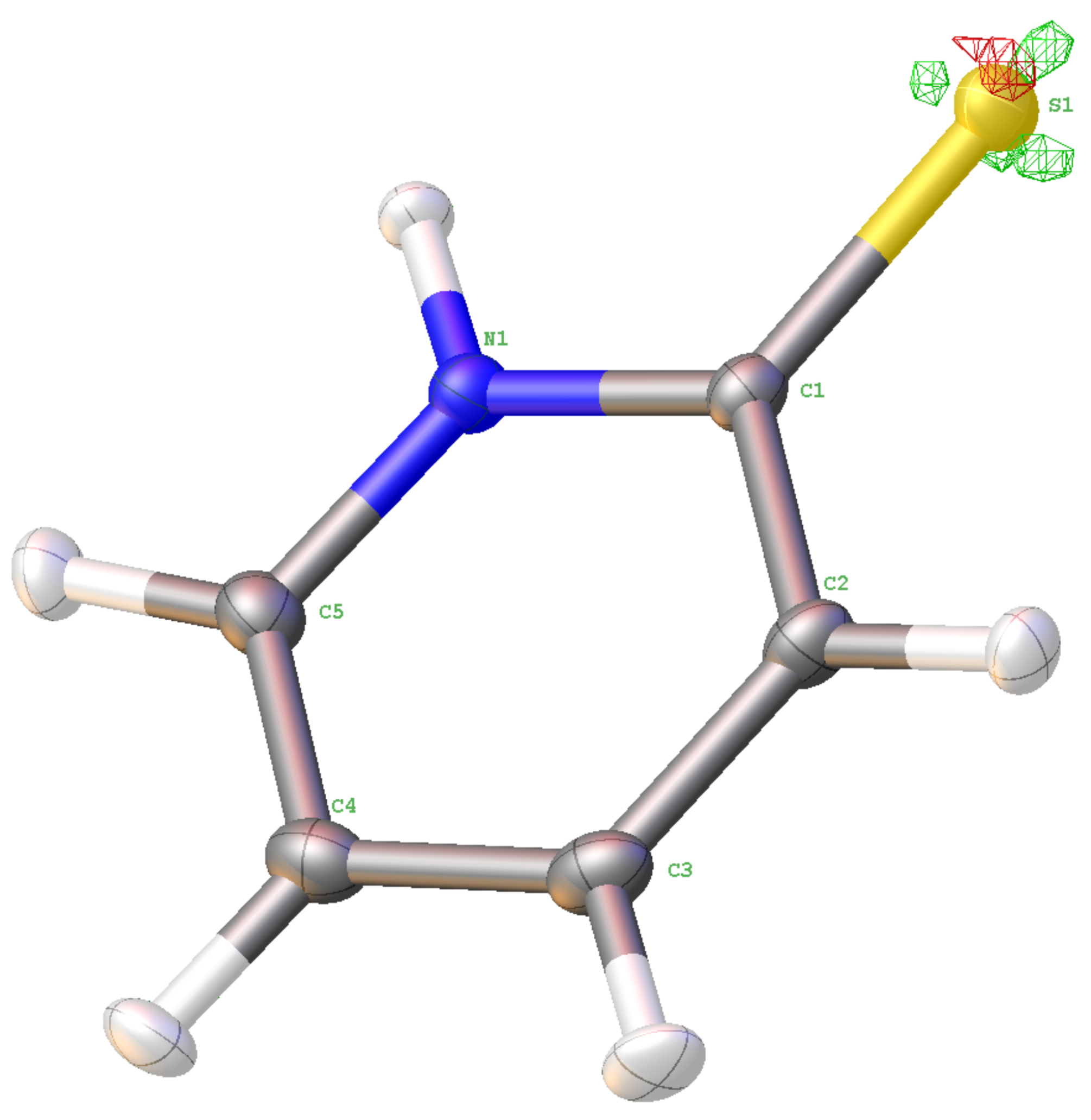
Still, the residual electron density map of (I) is not clean. What remains is non-random density at the sulfur atom. Because all electronic effects in the chemical bonds and the lone pairs should have been properly modeled by the non-spherical scattering factors, we speculate that the current harmonic model for the thermal motion is not sufficient. Anharmonic motion of sulfur atoms has been described before in the literature. For example, the authors of [6] find “typical shashlik-like residual density patterns” if the anharmonic motion is only modeled with harmonic displacement parameters. This is in contrast with the present case of (I), where there are four positive peaks at the sulfur in an approximately tetrahedral geometry. A possible explanation for the difference in the residual density pattern is a major difference in the crystal packing. (I) is involved in hydrogen bonding while the sulfur in [6] has no close intermolecular contacts. The different packing environment can certainly influence the atomic motion, resulting in a different residual density pattern when treated improperly (shashlik-like vs. tetrahedral). We also note that the packing in (I) is more dense than the packing in [6] (Tables S4 and S5).

If non-spherical scattering factors are used, hydrogen atoms can be refined with anisotropic displacement parameters and the results reach the accuracy of neutron diffraction [30]. In the present case of (I), the introduction of anisotropic displacement parameters for the hydrogen atoms improves the structural model significantly (Tables S6 and S7). A visualisation of the improvement is possible by comparing the calculated structure factors of the model with isotropic hydrogen atoms with those of anisotropic hydrogen atoms (Figure S7). Several reflections exceed the $3\sigma$ criterion.

Independent of the question about significance, we need to assess if the result is physically reasonable or not. The N–H distance is 1.035(3) Å, and the C–H distances are in the range 1.076(3)–1.084(3) Å. This corresponds very much to the expected values for neutron distances (1.020 and 1.085 Å, for N–H and C–H bonds [31]). From a peanut plot (Figure S8), the anisotropic parameters of the hydrogen atoms appear exaggerated. Still, the anisotropic hydrogen atoms from the NoSpherA2 result can be a starting point for the further steps of the analysis.

3.4. Multipole Refinement

The quality of the diffraction data allowed a multipole refinement. This approach is based on the Hansen–Coppens formalism [32] to describe the electron density by a combination of spherical harmonics and the expansion parameters $\kappa$ and ${\kappa }^{\prime }$. Essentially, it is a partitioning of the whole electron density into three parts: core density, spherical valence density and aspherical valence density:

$$\rho \left(r\right)=P_c{\rho }_c\left(r\right)+P_v{\kappa }^3{\rho }_v\left(\kappa r\right)+\sum _{l=0}^{l_{max}}{\kappa \prime }^3{R}_l\left({\kappa }^{\prime }r\right)\sum _{m=0}^l{P}_{lm\pm }{d}_{lm\pm }(\theta ,\varphi ).$$

For the multipole refinement, we used the XD software [15]. When parameters up to the hexadecapole level are used, similar agreement factors are reached as in the Hirshfeld atom refinement with NoSpherA2 in Olex2 (vide supra). Similarly, we again see non-random residual electron density close to the sulfur atom (Figure S9).

In a next step, anharmonic motion parameters for the sulfur atom were introduced with a third-order Gram–Charlier expansion as implemented in the XD software. This led to a significant improvement according to the Hamilton R-ratio test [7,33] (Table S8). It was even possible to add the anharmonic motion parameters to all non-hydrogen atoms. The refined expansion coefficients are 1.9–28.6 $\sigma$ for S, 0.3–6.3 $\sigma$ for N, and 0.0–9.5 $\sigma$ for C.

Following an idea from the literature [34], the anisotropic displacement parameters of the hydrogen atoms were refined freely. In this step, the hydrogen positions were kept fixed at the coordinates from the Hirshfeld atom refinement. Quadrupole parameters for the hydrogen atoms were included. Similar to the literature results [34], the resulting displacement parameters for hydrogen become smaller than from the Hirshfeld atom refinement and are physically more plausible (Figure S10). The residual density of this last refinement model with anharmonic motion parameters for the non-hydrogen atoms and refined anisotropic parameters for the hydrogen atoms is featureless, as can be seen in the map (Figure S11) and the fractal dimension plot (Figure S12).

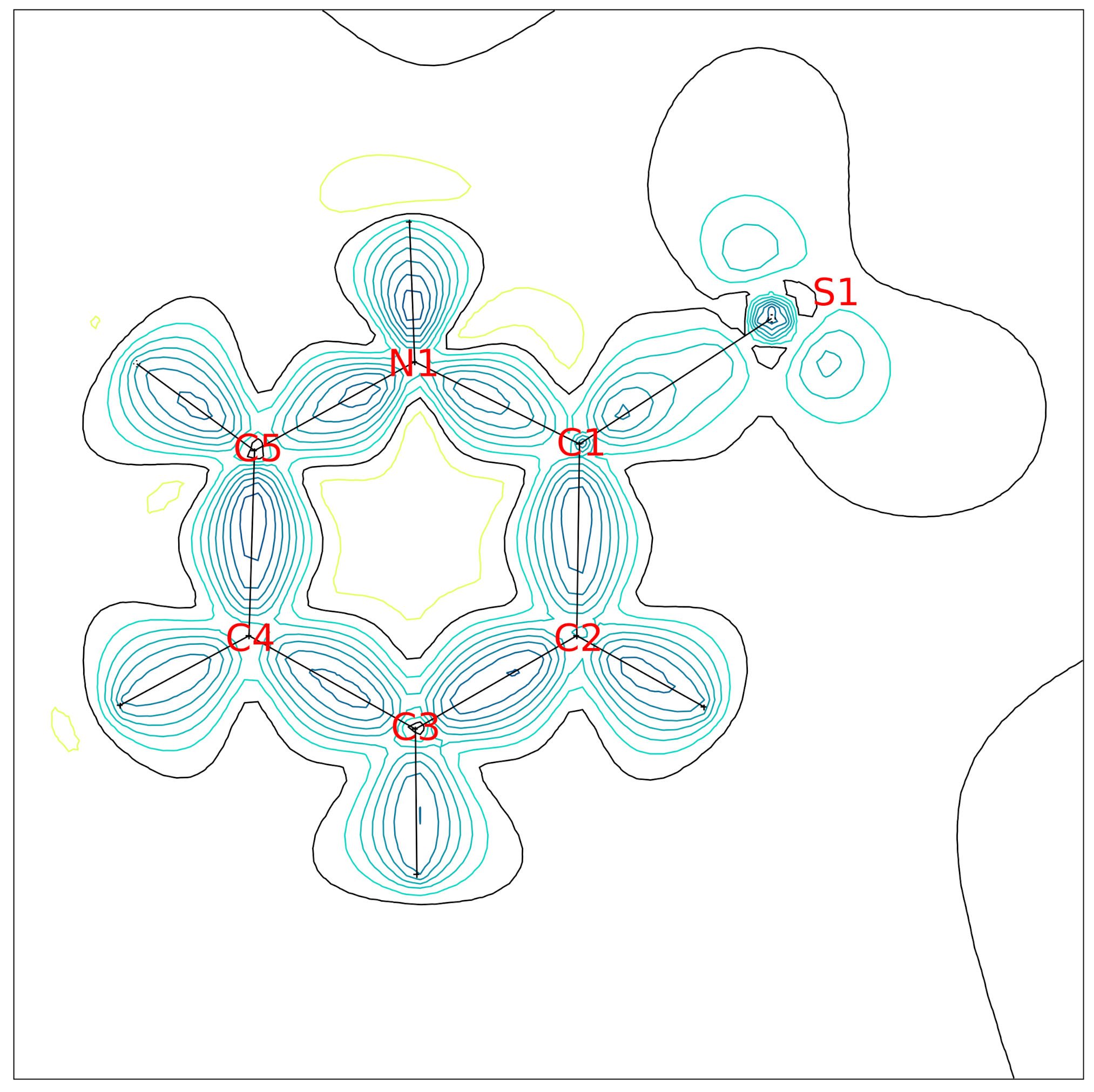
Figure 8 shows the deformation density in (I). This is a very clean map and none of the unexplainable features from [4] remain. In contrast to the X–N map of [4], we do not detect a negative residual density on the sulfur position; and in our map, the free electron pairs of the sulfur are visible. There are several potential explanations for this improvement. First of all, the study of [4] was an X-ray/neutron study (X–N study) while the current investigation is based on X-ray data only. X–N studies have several advantages and they are still very valuable today. A major disadvantage is that the diffraction experiments in X–N studies are usually performed on two different crystals. The crystal size and the crystal quality then differ and can result in scaling problems [35]. We also believe that our lowering of the temperature to 100 K compared to the literature study at room temperature helped to improve the results. Additionally, the redundancy of the reflections in (I) is rather high ($\mathrm{114,524}/8374=13.7$) compared to the literature study with a redundancy of $\mathrm{11,142}/1224=9.1$ for X-rays and $2547/1080=2.4$ for neutrons. A higher redundancy gives more reliable intensities and standard uncertainties. Finally, we detected anharmonic behaviour in (I) and included Gram–Charlier parameters in the refinement. The resolution in [4] was too low for such a treatment.

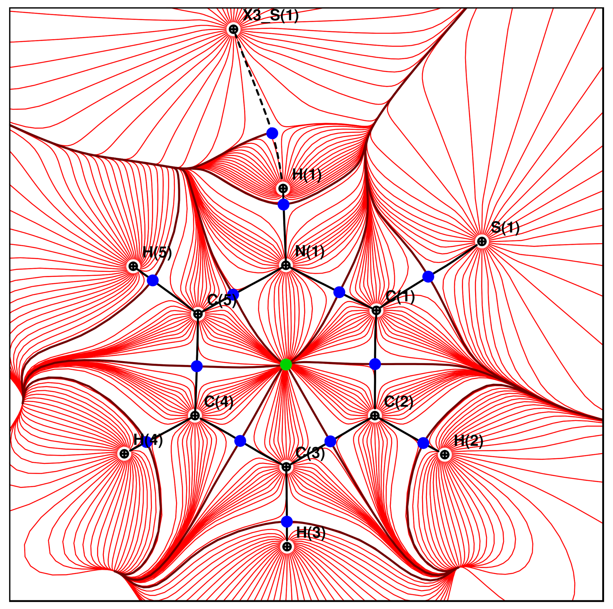
The deformation density is obtained by subtracting a promolecule based on spherical, independent atoms from the complete electron density. The choice of the promolecule brings some arbitrariness into the analysis and it is therefore now common practice to consider the total electron density [36,37]. A very popular procedure is the topological analysis according to Bader’s theory of Atoms in Molecules [38]. A trajectory plot of the electron density is shown in Figure 9 and an analysis of the (3, −1) critical points is listed in

Table 5. Topological analysis of the bond critical points ${\mathbf{r}}_{CP}$ in (I). $\rho$ is the electron density, ${\lambda }_1,{\lambda }_2\mathrm{and}{\lambda }_3$ are the eigenvalues of the Hessian matrix. $ϵ$ is the bond ellipticity. Symmetry codes i: $-x,1-y,-z$; ii: $x-1,y,z$.

Bond A–B	$\mathit{\rho }\left({\mathit{r}}_{\mathbf{CP}}\right)$ [eÅ${}^{-3}$]	${\mathit{\nabla }}^2\mathit{\rho }\left({\mathit{r}}_{\mathbf{CP}}\right)$ [eÅ${}^{-5}$]	${\mathit{\lambda }}_1$ [eÅ${}^{-5}$]	${\mathit{\lambda }}_2$ [eÅ${}^{-5}$]	${\mathit{\lambda }}_3$ [eÅ${}^{-5}$]	$\mathit{ϵ}$
S1–C1	1.459(8)	−5.24(2)	−8.19	−7.55	10.50	0.08
N1–C5	2.280(16)	−25.71(7)	−19.83	−16.91	11.03	0.17
N1–C1	2.233(12)	−24.47(6)	−19.45	−16.63	11.61	0.17
C1–C2	2.079(11)	−17.44(4)	−16.37	−13.45	12.38	0.22
C2–C3	2.227(13)	−20.64(4)	−17.59	−14.82	11.77	0.19
C3–C4	2.078(13)	−18.97(4)	−16.19	−14.40	11.62	0.12
C4–C5	2.284(13)	−22.49(4)	−18.92	−14.98	11.42	0.26
H1–S1${}^i$	0.172(6)	1.009(8)	−0.84	−0.72	2.57	0.17
H5–S1${}^{ii}$	0.062(4)	0.597(2)	−0.22	−0.15	0.96	0.44

and

Table 6. Locations of the bond critical points ${\mathbf{r}}_{CP}$ in (I). Symmetry codes i: $-x,1-y,-z$; ii: $x-1,y,z$.

Bond A–B	A–B [Å]	A–${\mathit{r}}_{\mathbf{CP}}$ [Å]	${\mathit{r}}_{\mathbf{CP}}$–B [Å]
S1–C1	1.6995(3)	0.8652	0.8343
N1–C5	1.3551(4)	0.8142	0.5409
N1–C1	1.3621(4)	0.8056	0.5565
C1–C2	1.4188(3)	0.7239	0.6950
C2–C3	1.3783(5)	0.6932	0.6852
C3–C4	1.4111(5)	0.7134	0.6978
C4–C5	1.3702(4)	0.6654	0.7049
H1–S1${}^i$	2.2712	0.7684	1.5029
H5–S1${}^{ii}$	2.8604	1.1154	1.7451

. The bond lengths alternation discussed above is also seen in the Laplacian values and is thus consistent with the strengths of these covalent bonds. In addition, it was possible to detect the bond critical point for the intermolecular N–H⋯S hydrogen bond. Comparing the Laplacian value at this critical point with earlier studies [39], it becomes clear that the N–H⋯S hydrogen bond is much weaker than typical O–H⋯O and most N–H⋯O hydrogen bonds. In another example, Laplacian values of 3.398 and 3.303 eÅ${}^{-5}$ were found at the critical points of O–H⋯N hydrogen bonds in an oxime [40]. It is thus surprising that the weak N–H⋯S hydrogen bond in (I) results in only little thermal expansion over a wide temperature range.

The search for bond critical points delivers an additional intermolecular interaction which has not come forward in the geometrical discussion above. It is between the C5–H5 group and the sulfur atom. Considering the thermal expansion of this contact (Table S9), it has similar behaviour and strength as the described $\pi \cdots \pi$ stacking. This C–H⋯S interaction is in the crystallographic a-direction and should thus connect the layers depicted in Figure 4. Considering the enrichment ratios in Table 3 which show that H⋯S contacts are favorable, the C5–H5⋯S1 contact might stabilize the crystal packing.

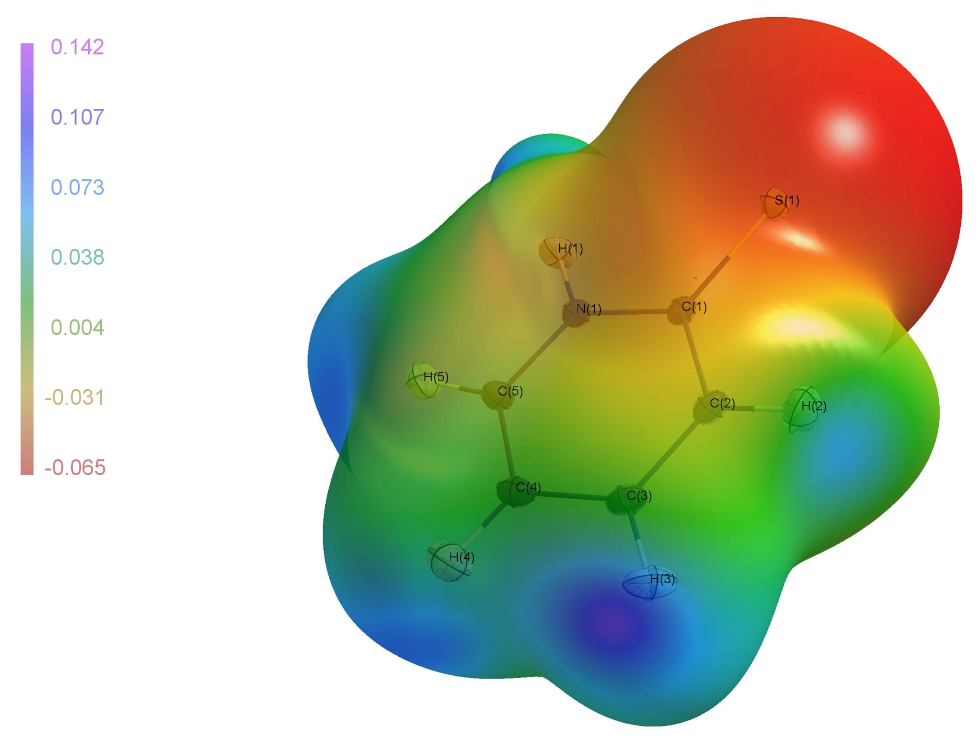
The electrostatic potential which was derived from the experimental electron density (Figure 10) shows that negative regions are on the sulfur atom S1, while the positive regions are on the hydrogen atoms. By looking at the crystal packing with this picture in mind, we can state qualitatively that only the N–H⋯S hydrogen bond has an electrostatic character. Other attractive intermolecular forces in (I) will have a dispersive nature.

4. Conclusions

As a planar molecule, (I) has approximate mirror symmetry. This symmetry is not fulfilled by the crystal environment. The two sides of the molecule have different intermolecular interactions, resulting in a non-symmetric crystal field. As a consequence, the thermal expansion in a wide temperature range indicates anharmonic behaviour. Anharmonic behaviour was also detected in the atomic displacement parameters. Only the inclusion of anharmonic parameters (Gram–Charlier expansion) leads to a clean residual density map, especially at the sulfur atom. From this final model, a deformation density map was derived which no longer shows the uncommon features from an earlier study in the literature [4].

References

1. Moran, D.; Sukcharoenphon, K.; Puchta, R.; Schaefer, H.F.; Schleyer, P.V.R.; Hoff, C.D. 2-Pyridinethiol/2-Pyridinethione Tautomeric Equilibrium. A Comparative Experimental and Computational Study. J. Org. Chem. 2002, 67, 9061–9069. [Google Scholar] [CrossRef] [PubMed]
2. Van Kuiken, B.E.; Ross, M.R.; Strader, M.L.; Cordones, A.A.; Cho, H.; Lee, J.H.; Schoenlein, R.W.; Khalil, M. Picosecond sulfur K-edge X-ray absorption spectroscopy with applications to excited state proton transfer. Struct. Dyn. 2017, 4, 044021. [Google Scholar] [CrossRef] [PubMed] [Green Version]
3. Penfold, B.R. The crystal structure of α-thiopyridone. Acta Crystallogr. 1953, 6, 707–713. [Google Scholar] [CrossRef] [Green Version]
4. Ohms, U.; Guth, H.; Kutoglu, A.; Scheringer, C. 2-Thiopyridone: X-ray and neutron diffraction study. Acta Crystallogr. Sect. B 1982, 38, 831–834. [Google Scholar] [CrossRef]
5. Reynolds, J.G.; Sendlinger, S.C.; Murray, A.M.; Huffman, J.C.; Christou, G. Synthesis and Characterization of Vanadium(II,III,IV) Complexes of Pyridine-2-thiolate. Inorg. Chem. 1995, 34, 5745–5752. [Google Scholar] [CrossRef]
6. Herbst-Irmer, R.; Henn, J.; Holstein, J.J.; Hübschle, C.B.; Dittrich, B.; Stern, D.; Kratzert, D.; Stalke, D. Anharmonic Motion in Experimental Charge Density Investigations. J. Phys. Chem. A 2013, 117, 633–641. [Google Scholar] [CrossRef]
7. Destro, R.; Roversi, P.; Barzaghi, M.; Lo Presti, L. Anharmonic Thermal Motion Modelling in the Experimental XRD Charge Density Determination of 1-Methyluracil at T = 23 K. Molecules 2021, 26, 3075. [Google Scholar] [CrossRef]
8. Schreurs, A.M.M.; Xian, X.; Kroon-Batenburg, L.M.J. EVAL15: A diffraction data integration method based on ab initio predicted profiles. J. Appl. Crystallogr. 2010, 43, 70–82. [Google Scholar] [CrossRef]
9. Krause, L.; Herbst-Irmer, R.; Sheldrick, G.M.; Stalke, D. Comparison of silver and molybdenum microfocus X-ray sources for single-crystal structure determination. J. Appl. Crystallogr. 2015, 48, 3–10. [Google Scholar] [CrossRef] [Green Version]
10. Kleemiss, F.; Dolomanov, O.V.; Bodensteiner, M.; Peyerimhoff, N.; Midgley, L.; Bourhis, L.J.; Genoni, A.; Malaspina, L.A.; Jayatilaka, D.; Spencer, J.L.; et al. Accurate crystal structures and chemical properties from NoSpherA2. Chem. Sci. 2021, 12, 1675–1692. [Google Scholar] [CrossRef]
11. Sun, Q.; Berkelbach, T.C.; Blunt, N.S.; Booth, G.H.; Guo, S.; Li, Z.; Liu, J.; McClain, J.D.; Sayfutyarova, E.R.; Sharma, S.; et al. PySCF: The Python-based simulations of chemistry framework. WIREs Comput. Mol. Sci. 2018, 8, e1340. [Google Scholar] [CrossRef]
12. Sheldrick, G.M. Crystal structure refinement with SHELXL. Acta Crystallogr. Sect. C 2015, 71, 3–8. [Google Scholar] [CrossRef]
13. Dolomanov, O.V.; Bourhis, L.J.; Gildea, R.J.; Howard, J.A.K.; Puschmann, H. OLEX2: A complete structure solution, refinement and analysis program. J. Appl. Crystallogr. 2009, 42, 339–341. [Google Scholar] [CrossRef]
14. Sheldrick, G.M. XPREP, Version 2008/2; Bruker AXS Inc.: Madison, WI, USA, 2008.
15. Volkov, A.; Macchi, P.; Farrugia, L.J.; Gatti, C.; Mallinson, P.R.; Richter, T.; Koritsanszky, T. XD2016, Version 2016.01. A Computer Program for Multipole Refinement, Topological Analysis of Charge Densities and Evalution of Intermolecular Interaction Energies from Experimental or Theoretical Structure Factors. 2016.
16. Grimme, S. Do Special Noncovalent ππ Stacking Interactions Really Exist? Angew. Chem. Int. Ed. 2008, 47, 3430–3434. [Google Scholar] [CrossRef]
17. Takahashi, O.; Nishio, M. The CH/⋯π Hydrogen Bond. In Intermolecular Interactions in Crystals: Fundamentals of Crystal Engineering; Novoa, J.J., Ed.; The Royal Society of Chemistry: London, UK, 2018; pp. 453–477. [Google Scholar]
18. Nishio, M. The CH/π hydrogen bond: Implication in chemistry. J. Mol. Struct. 2012, 1018, 2–7. [Google Scholar] [CrossRef]
19. Kumar, M.; Balaji, P.V. C-H⋯π interactions in proteins: Prevalence, pattern of occurrence, residue propensities, location, and contribution to protein stability. J. Mol. Model. 2014, 20, 2136. [Google Scholar] [CrossRef]
20. Spek, A.L. Structure validation in chemical crystallography. Acta Crystallogr. Sect. D 2009, 65, 148–155. [Google Scholar] [CrossRef]
21. Spackman, P.R.; Turner, M.J.; McKinnon, J.J.; Wolff, S.K.; Grimwood, D.J.; Jayatilaka, D.; Spackman, M.A. CrystalExplorer: A program for Hirshfeld surface analysis, visualization and quantitative analysis of molecular crystals. J. Appl. Crystallogr. 2021, 54, 1006–1011. [Google Scholar] [CrossRef]
22. Jelsch, C.; Ejsmont, K.; Huder, L. The enrichment ratio of atomic contacts in crystals, an indicator derived from the Hirshfeld surface analysis. IUCrJ 2014, 1, 119–128. [Google Scholar] [CrossRef]
23. Schomaker, V.; Trueblood, K.N. Correlation of Internal Torsional Motion with Overall Molecular Motion in Crystals. Acta Crystallogr. Sect. B 1998, 54, 507–514. [Google Scholar] [CrossRef] [Green Version]
24. Hirshfeld, F.L. Can X-ray data distinguish bonding effects from vibrational smearing? Acta Crystallogr. Sect. A 1976, 32, 239–244. [Google Scholar] [CrossRef]
25. Lovett, D.R. Tensor Properties of Crystals, 2nd ed.; Institute of Physics Publishing: Bristol, UK, 1999. [Google Scholar]
26. Ohashi, Y. A Program to Calculate the Strain Tensor from Two Sets of Unit-cell Parameters. In Comparative Crystal Chemistry; Hazen, R.M., Finger, L.W., Eds.; Wiley: Chichester, UK, 1982; pp. 92–102. [Google Scholar]
27. Bürgi, H.B.; Capelli, S.C.; Birkedal, H. Anharmonicity in anisotropic displacement parameters. Acta Crystallogr. Sect. A 2000, 56, 425–435. [Google Scholar] [CrossRef]
28. Salud, J.; Barrio, M.; López, D.O.; Tamarit, J.L.; Alcobé, X. Anisotropy of Intermolecular Interactions from the Study of the Thermal-Expansion Tensor. J. Appl. Crystallogr. 1998, 31, 748–757. [Google Scholar] [CrossRef] [Green Version]
29. Meindl, K.; Henn, J. Foundations of residual-density analysis. Acta Crystallogr. Sect. A 2008, 64, 404–418. [Google Scholar] [CrossRef]
30. Capelli, S.C.; Bürgi, H.B.; Dittrich, B.; Grabowsky, S.; Jayatilaka, D. Hirshfeld atom refinement. IUCrJ 2014, 1, 361–379. [Google Scholar] [CrossRef] [Green Version]
31. Allen, F.H.; Bruno, I.J. Bond lengths in organic and metal-organic compounds revisited: X–H bond lengths from neutron diffraction data. Acta Crystallogr. Sect. B 2010, 66, 380–386. [Google Scholar] [CrossRef]
32. Hansen, N.K.; Coppens, P. Testing aspherical atom refinements on small-molecule data sets. Acta Crystallogr. Sect. A 1978, 34, 909–921. [Google Scholar] [CrossRef]
33. Hamilton, W.C. Significance tests on the crystallographic R Factor. Acta Crystallogr. 1965, 18, 502–510. [Google Scholar] [CrossRef]
34. Köhler, C.; Lübben, J.; Krause, L.; Hoffmann, C.; Herbst-Irmer, R.; Stalke, D. Comparison of different strategies for modelling hydrogen atoms in charge density analyses. Acta Crystallogr. Sect. B 2019, 75, 434–441. [Google Scholar] [CrossRef] [PubMed] [Green Version]
35. Blessing, R.H. On the differences between X-ray and neutron thermal vibration parameters. Acta Crystallogr. Sect. B 1995, 51, 816–823. [Google Scholar] [CrossRef] [PubMed]
36. Koritsanszky, T.S.; Coppens, P. Chemical Applications of X-ray Charge-Density Analysis. Chem. Rev. 2001, 101, 1583–1628. [Google Scholar] [CrossRef]
37. Gatti, C. Chemical bonding in crystals: New directions. Z. Kristallogr. Cryst. Mater. 2005, 220, 399–457. [Google Scholar] [CrossRef]
38. Bader, R.F.W. Atoms in Molecules: A Quantum Theory; Clarendon Press: Oxford, UK, 1990. [Google Scholar]
39. Espinosa, E.; Souhassou, M.; Lachekar, H.; Lecomte, C. Topological analysis of the electron density in hydrogen bonds. Acta Crystallogr. Sect. B 1999, 55, 563–572. [Google Scholar] [CrossRef]
40. Marsman, A.W.; van Walree, C.A.; Havenith, R.W.A.; Jenneskens, L.W.; Lutz, M.; Spek, A.L.; Lutz, E.T.G.; van der Maas, J.H. Infinite, undulating chains of intermolecularly hydrogen bonded (E,E)-2,2-dimethylcyclohexane-1,3-dione dioximes in the solid state. A single crystal X-ray, charge density distribution and spectroscopic study. J. Chem. Soc. Perkin Trans. 2 2000, 3, 501–510. [Google Scholar] [CrossRef]
41. Hübschle, C.B.; Dittrich, B. MoleCoolQt—A molecule viewer for charge-density research. J. Appl. Crystallogr. 2011, 44, 238–240. [Google Scholar] [CrossRef] [Green Version]
Scheme 1. Tautomeric forms of 2-mercaptopyridone: thiopyridone form (left) and thiolpyridine form (right).
Crystals 12 00338 sch001
Figure 1. Hydrogen-bonded dimer in the crystal structure of (I). Result of the SHELXL refinement. Displacement ellipsoids are drawn at the 50% probability level. Symmetry code i: x , 1 y , z . N1–H1 0.873(7), H1 S 1 i 2.414(7), N1 S 1 i 3.27197(16) Å. N1–H1 S 1 i 167.7(6) .
Crystals 12 00338 g001
Figure 2. Weak intermolecular interactions in the crystal structure of (I). Projection along the crystallographic a axis. N–H⋯S hydrogen bonds, antiparallel π π stacking and C–H π interactions are shown as dashed lines.
Crystals 12 00338 g002
Figure 3. (Left) Hirshfeld surface of (I) as calculated with CrystalExplorer (version 21.5) [21]. The colour of the surface is determined by the normalized contact distance d n o r m = d | e | + d | i | . (Right) Fingerprint plot derived from the Hirshfeld surface; d i is the interior and d e the exterior distance.
Crystals 12 00338 g003
Figure 4. Two-dimensional layers formed by weak intermolecular interactions in the b , c plane are stacked in the direction of the a axis. The intermolecular interactions are drawn as dashed lines. The ellipsoid of the anisotropic thermal expansion tensor is drawn on an arbitrary scale.
Crystals 12 00338 g004
Figure 5. Temperature-dependent development of the unit cell volume. The quadratic fit results in the equation y = 513.54 + 0.062073 × x + 8.4949 × 10 5 × x 2 .
Crystals 12 00338 g005
Figure 6. Temperature-dependent development of the equivalent isotropic displacement parameters U e q . The lines were obtained by quadratic fits, respectively. U e q = 1 3 i , j U i j a i a j a i · a j .
Crystals 12 00338 g006
Figure 7. Difference electron density in (I). Contour level 0.217 e/Å 3 . Positive contours are drawn in green, negative in red. Calculated structure factors are taken from the non-spherical atom model refined with NoSpherA2 [10] in Olex2 [13]. Maximum resolution ( sin θ / λ ) m a x = 1.24 Å 1 . Plot prepared with Olex2.
Crystals 12 00338 g007
Figure 8. Static deformation density in (I) from the final multipole refinement. Contour level 0.1 e/Å 3 .
Crystals 12 00338 g008
Figure 9. Trajectory plot of the electron density in (I) from the final multipole refinement. (3, −1) Critical points are drawn as blue circles and the (3, +1) critical point as a green circle. The intermolecular N–H⋯S hydrogen bond is drawn with dashed lines. The drawing was created with the module XDPROP of the XD software [15].
Crystals 12 00338 g009
Figure 10. Isosurface of the electron density at 0.001 au. Mapped on this surface is the electrostatic potential. For the meaning of the colours, see the legend in the inset. Three-dimensional grids were calculated with the module XDPROP in XD [36]. The plot was prepared with MoleCoolQt [41].
Crystals 12 00338 g010