Numerical Simulation of the Effect of Wall-Equiaxed Crystal Density on the Number of Columnar Crystals and the Thickness of an Equiaxed Crystal Layer for Al-4.7%Cu Alloy Ingot Based on 3D LBM-CA Method

Abstract

In this paper, the lattice Boltzmann–cellular automata (LBM-CA) model with dynamic and static grids was used to study the growth of three-dimensional (3D) multidendrites under directional solidification with random preferred angles. In the static grid, the temperature field, flow field, and solute field during solidification were calculated by the LBM method, and in the dynamic grid, each dendrite evolution was calculated based on the CA method at its preferential crystallographic orientation. The coupling of LBM and CA was made by interpolation of the correlation quantities between the two sets of grids. The effects of wall-equiaxed crystal density on the number of columnar crystals and the thickness of the equiaxed crystal layer were studied by this model. The results showed that the density of the wall-equiaxed crystal has little effect on the number of columnar crystals and the thickness of the equiaxed crystal layer. When other conditions were the same, the lower the undercooling, the fewer the columnar crystals, and the thicker the equiaxed layer. In addition, the smaller the heat transfer coefficient, the lower the number of columnar grains, and the smaller the thickness of equiaxed grains.

1. Introduction

In the study of dendrite growth, it is difficult to observe details of the growth process. With the rapid development of computer techniques, it is becoming increasingly important to study the solidification process by numerical methods combined with verification. The lattice Boltzmann method (LBM) has been a popular method for computing fluids in recent years. Compared with other methods [1,2], the LBM algorithm has the advantages of being a simple algorithm with a high computational efficiency, easy-to-handle complex boundary, and good stability [3,4]. The CA method [5] has a certain physical background, it has the characteristics of being a simple program with flexible calculation in simulating dendrite growth, and it has great potential in simulating the calculation of the solidification structure [6,7]. The advantages of the two methods can be developed by coupling the two methods, which has great potential and advantages in solidification structure simulation.

There have been many papers on the two-dimensional (2D) numerical simulation of dendrite growth by the CA method [8,9,10], but the morphology of dendrites is 3D [11], and the results based on 2D calculation cannot fully reflect the true dendritic morphology, so it is impossible to investigate the effect of preferential crystallographic orientation and grain density on the growth morphology of columnar crystals.

In recent years, the numerical simulation of the 3D dendrite growth process has also gradually become in-depth. Brown et al. [12,13] established a 3D CA coupled finite difference (FD) method model to predict the eutectic growth of two phases. Wang et al. [14] combined CA with the finite element method (FE) to predict the selection of primary dendrite arm spacings and simulate the growth of 3D equiaxed crystals and columnar crystals. Zhang et al. [15] established a 3D CA model for dendrite growth of a multicomponent alloy, and they verified the correctness of the model by comparison with the theoretical prediction of a ternary alloy. Xu et al. [16] established a 3D CA model for the evolution of the aluminum alloy solidification process. Compared with the phase field method, the calculation time of this model is very short. Jiang et al. [17] established a 3D model for the dendrite growth of cubic metals and alloys by coupling CA with the FD method. The model can accurately describe the solidification structure evolution process of cubic metals and alloys. Wei et al. [18] used 3D adaptive mesh refinement technology coupled with the CA model to simulate the morphology of 3D equiaxed dendrites of pure materials, and they studied the influence of the interface energy anisotropy coefficient on the 3D grain morphology. Pan et al. [19] established a sharp interface model of the 3D CA method and quantitatively simulated the growth of dendrites, and they calculated the growth morphology of 3D equiaxed dendrites with different crystallographic orientations. Chen et al. [20] eliminated the anisotropy of the mesh through the eccentric algorithm, and established an improved CA model, which is suitable for the calculation of the 2D and 3D growth of dendrites. Gu et al. [21,22] established a 3D quantitative CA model for dendrite growth during the solidification of a ternary alloy, which can accurately predict the dendrite morphology and solute distribution of equiaxed dendrites and columnar crystals during solidification. Pian [23] established a 3D CA model to simulate a single-phase solid solution alloy. This model can calculate the growth of regular dendrites under natural convection but cannot calculate the evolution of dendrites with preferential angles, which is obviously inconsistent with the actual situation.

Among the numerous research studies on 3D dendrite growth numerical simulation, the research on 3D equiaxed-columnar transformation mainly includes Wang and Lee [14], Wei et al. [24], Pan and Zhu [19], Eshraghi and Felicelli [25], and Gu et al. [22]. Among them, only Wang and Lee have studied the effect of the density of wall-equiaxed crystals on the distribution and morphology of columnar crystals, but their calculation assumes that the preferred growth direction of wall-equiaxed crystals is parallel to the coordinate axis. They did not study the case when the preferred growth direction of wall-equiaxed crystals is random, but the actual situation is random. Wei’s CET calculation is similar to Wang’s, and the wall-equiaxed crystal also grows in the positive direction. Pan and Zhu, Eshraghi and Felicelli, and Gu all calculated the wall-equiaxed crystals with random preferred orientations, but they did not study the effect of the growth of wall-equiaxed crystals with random preferred orientations on the morphology of columnar crystals. In addition, the effect of natural convection on dendrite growth was not calculated in the above numerical simulation.

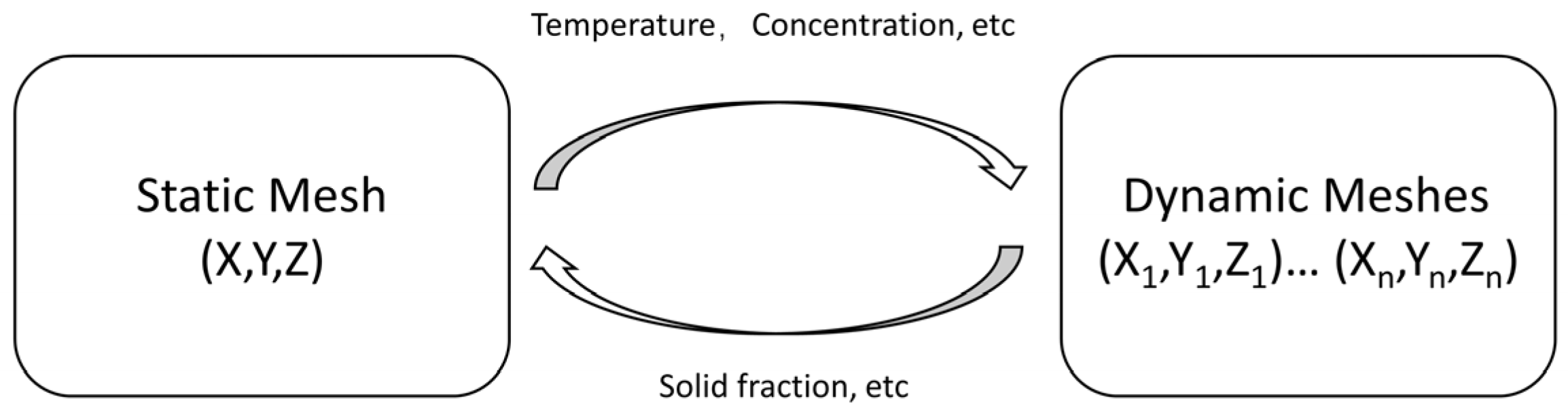
It can be seen from the above that the 3D numerical simulation of dendrite growth has made some progress, but research on the 3D numerical simulation of dendrite competitive growth evolution with random preferential angles under the influence of directional heat flux has hardly been reported, and the influence of equiaxed crystal density on the number of columnar crystals has rarely been studied. However, this is a scientific question that needs to be answered in general ingot solidification or directional solidification. In this paper, a three-dimensional LBM-CA coupling model based on two sets of meshes was established. By setting two sets of meshes, the three fields (temperature field, flow field, and solute field) and the growth and capture of dendrites in the calculation area were separately carried out in two sets of grids. On the basis of this model, the effects of the grain density of wall-equiaxed grains on the number of columnar grains and the thickness of the equiaxed layer under the action of directional heat flux were calculated and studied.

2. Materials and Methods

We selected the Al-4.7wt%Cu alloy as the simulation research material, and its physical parameters are listed in

Table 1. Physical properties of Al-4.7wt%Cu alloy.

Physical Parameter	Symbol	Value
Liquidus temperature	TL[K]	917
Solidus temperature	TS[K]	821
Liquidus slope	m[m·K/%]	−3.44
Thermal diffusivity	α[W·m−1 K−1]	3 × 10−8
Interface anisotropy coefficient	ε	0.05
Diffusivity in liquid	D[m2·s−1]	3.0 × 10−9
Partition coefficient	k	0.145
Kinematic viscosity	ν[m2·s−1]	9 × 10−9
Temperature expansion coefficient	βT	1 × 10−2
Concentration expansion coefficient	βC	1 × 10−3

. Detailed symbol abbreviations can be found in

Table A1. Detailed list of symbol abbreviations used in this paper with brief explanations.

Symbols	Unit	Meaning
fs	mass%	Solid fraction
CL	mass%	Actual solute concentration at interface
CLeq	mass%	Liquid-phase equilibrium crystallization concentration at the interface
Δfs	mass%	Solid fraction increment
k	—	Equilibrium partition coefficient of solute
C0	mass%	Initial concentration of the alloy
TL	K	Actual temperature of the interface
TLeq	K	Equilibrium liquidus temperature
m	k/mass%	Liquidus slope
Γ	m·K	Gibbs–Thomson coefficient
K	1/m	Average curvature at the solid/liquid interface
ε	—	Anisotropic strength of interface energy
τf	—	Relaxation time of flow field
τα	—	Relaxation time of temperature field
τD	—	Relaxation time of concentration field
ν	m2/s	Fluid viscosity
α	m2/s	Thermal diffusivity
D	m2/s	Concentration diffusion coefficient
ρ0	Kg/m3	Initial density of fluid
T0	K	Initial temperature
βT	K−1	Volume expansion coefficient of temperature change
βC	Mass%−1	Volume expansion coefficient of concentration change
ωi	—	Weight coefficient
ei	m/s	Discrete velocity
c	m/s	Lattice velocity
g	m/s2	Gravitational acceleration
F	N	The force of fluid on dendrite
Fi	N	The component force of the particle in the i direction
Gi	mass%	Source term of concentration field
Hi	K	Source term of temperature field
u	m/s	Macroscopic velocity
ΔT	K	Undercooling

in Appendix A.

2.1. LBM Model

In this paper, the D3Q15 model [5] was selected to calculate the three-dimensional flow field, and the evolution equation of the distribution function [10] can be described as follows:

f_i(x + e_iΔt, t + Δt) − f_i(x, t) = (f_i^eq(x, t) − f_i(x, t))/τ_f + F_i

(1)

where f_i(x, t) is the distribution function, which represents the probability of particles appearing in position x and time t. f_i^eq(x, t) is the equilibrium distribution function, e_i is the particle velocity in the direction i, Δt is the time step, and τ_f is the flow field relaxation time. f_i^eq(x, t) can be calculated by

f_i^eq(x, t) = ω_iρ(1 + 3e_i·u/(c²) + 9(e_i·u)²/(2c⁴) − 3(u·u)/(2c²))

(2)

where c is the lattice velocity and ω_i is the weight coefficient. When I = 0, ω_i = 16/72; when I = 1~6, ω_i = 8/72; when I = 7~14, ω_i = 1/72.

The relationship between τ_f and viscosity ν can be expressed as

τ_f = 3ν/(c²Δt) + 0.5

(3)

where F is the buoyancy that produces natural convection. According to the Boussinesq approximation, the density in the buoyancy term is a linear function of temperature gradient and concentration gradient and can be calculated by

F = gρ₀β_T(T − T₀) + gρ₀β_C (C − C₀)

(4)

where ρ₀ is the initial density of the fluid, T is the current temperature, T₀ is the initial temperature, C is the current concentration, C₀ is the initial concentration, β_T is the volume expansion coefficient of the temperature change, β_C is the volume expansion coefficient of the concentration change, and g is the gravity acceleration.

The density and velocity of the macroscopic physical quantity can be evaluated by

Ρ = ∑f_i

(5)

U = (e_if_i + F·Δt/2)/ρ

(6)

The calculation of the temperature field and concentration field is similar to that of the flow field. h_i(x, t) and g_i(x, t) are the distribution functions of temperature and concentration, respectively, and they can be calculated by

h_i(x + e_iΔt, t + Δt) = h_i(x, t) + (h_i^eq(x, t) − h_i(x, t))/τ_α + H_i

(7)

g_i(x + e_iΔt, t + Δt) = g_i(x, t) + (g_i^eq(x, t) − g_i(x, t))/τ_D + G_i

(8)

The equilibrium distribution functions corresponding to h_i(x, t) and g_i(x, t) can be calculated by

h_i^eq(x, t) = ω_iT(1 + 3e_i·u/(c²) + 9(e_i·u)²/(2c⁴) − 3(u·u)/(2c²))

(9)

g_i^eq(x, t) = ω_iC(1 + 3e_i·u/(c²) + 9(e_i·u)²/(2c⁴) − 3(u·u)/(2c²))

(10)

where H_i and G_i in the distribution function of temperature and concentration are the concentration and temperature source terms caused by solute redistribution and latent heat release during dendrite growth, respectively, which can be given by

G_i = ω_iC_l(1 − k)Δf_s

(11)

H_i = ω_iΔf_sL/c_P

(12)

Among them, k is the equilibrium distribution coefficient, L is the latent heat of solidification, c_P is the specific heat capacity, C_l is the composition in the liquid phase, and Δf_s is the increase in solid fraction of an interface cell in a time step. The relationships between temperature field relaxation time τ_α and thermal diffusion coefficient α, and concentration field relaxation time τ_D and solute diffusion coefficient D are as follows:

τ_α = 3α/(c²Δt) + 0.5

(13)

τ_D = 3D/(c²Δt) + 0.5

(14)

The macroscopic temperature and concentration of the fluid can be obtained by summing the corresponding distribution functions:

T = ∑h_i(x,t)

(15)

C = ∑g_i(x,t)

(16)

The boundary of the simulation domain and the SL interface of the flow field are treated by the nonslip bounce back. The boundary of the simulation area of the concentration field is the nondiffusion boundary, and the SL interface is treated by bounce back. The nonequilibrium extrapolation method is used to simulate the boundary of the temperature field, and the thermal conductivity is assumed to be the same at the SL interface.

2.2. CA Model

In this paper, the model proposed by Zhu et al. [19] was used for dendrite evolution. The driving force of dendrite evolution is controlled by the difference between the equilibrium concentration of the solute and the actual solute concentration at the interface. According to the interface equilibrium conditions, the increase in solid fraction of the growth cell can be calculated by

Δf_s = (C_l^eq − C_l)/(C_l^eq(1 − k))

(17)

Among them, k is the equilibrium partition coefficient, C_l is the actual solute concentration of the interfacial cell, and C_l^eq is the equilibrium solute concentration of the interfacial cell, which can be calculated by

C_l^eq = C₀ + (T − T^eq)/m + Γ·wmc/m

(18)

where T is the actual temperature of the interface cell, T^eq is the equilibrium liquidus temperature corresponding to the initial alloy concentration of C₀, m is the slope of the liquidus, Γ is the Gibbs–Thomson coefficient, and wmc is the 3D weighted mean curvature, which can be calculated by

wmc = (3ε − 1)(∂n_x/∂x + ∂n_y/∂y + ∂n_z/∂z) − 48ε(n_x²·∂n_x/∂x + n_y²·∂n_y/∂y + n_z²·∂n_z/∂z) + 12Qε(∂n_x/∂x + ∂n_y/∂y + ∂n_z/∂z) + 12ε(n_x·∂Q/∂x + n_y·∂Q/∂y + n_z·∂Q/∂z)

(19)

where ε is the anisotropic coefficient of interface energy, $n_x=\left(\partial f_s/\partial x\right)/\left|\nabla f_s\right|$, $n_y=\left(\partial f_s/\partial y\right)/\left|\nabla f_s\right|$,$n_z=\left(\partial f_s/\partial z\right)/\left|\nabla f_s\right|$, and $\left|\nabla f_s\right|={\left({\left(\partial f_s/\partial x\right)}^2+{\left(\partial f_s/\partial y\right)}^2+{\left(\partial f_s/\partial z\right)}^2\right)}^{1/2}$.

In this paper, a capture mode of 6 neighboring cells was used. Solid-state cells capture only 6 cells nearest to them.

2.3. Dynamic and Static Mesh Methods

2.3.1. Algorithm for Dendrite Growth Calculation by Dynamic and Static Meshes

In this paper, the dynamic and static meshes were used to calculate the dendrites with random preferential crystallographic orientations. The static mesh is set-up for the whole calculation domain, which is in the absolute coordinate system; a set of dynamic grids is set for each dendrite in the dynamic coordinate system, and the direction of the axes is parallel to the preferential orientation of the dendrite, therefore, the dendrite evolution is always regular in the dynamic coordinate system, and the size of the dynamic mesh changes dynamically with the evolution of the dendrite. The schematic diagram of the two meshes is shown in Figure 1.

The temperature field, solute field, and flow field are calculated in the absolute coordinate system by the LBM method. The interpolation method is used to transform the calculation results into a dynamic mesh, and the CA method is used to calculate dendrite evolution. Dendrites grow regularly in the dynamic coordinate system without considering the anisotropy of the mesh. In a time step, after the dendrite evolution is calculated, the calculation results are converted to the static mesh for the next cycle calculation. LBM and CA are independently used in the dynamic mesh and static mesh, respectively, where coordinate transformation and interpolation calculation are the links between them.

2.3.2. Coordinate Transformation between Static and Dynamic Meshes

Because the meshes of two coordinate systems are not a one-to-one correspondence, and the dynamic meshes are not necessarily within the static mesh, the coordinate of the dynamic mesh node (i, j, k) in the absolute coordinate system (i₂, j₂, k₂) should be considered in the calculation.

There is a certain coordinate relationship between dynamic mesh and static mesh. The position of dynamic mesh nodes in the static mesh can be obtained by coordinate transformation. Coordinate transformation is realized by the coordinate rotation matrices R₁, R₂, and R₃. These three coordinate rotation matrices are as follows:

$$R_1=\left[\begin{array}{ccc}\cos \left(angle\_z\right)& -\sin \left(angle\_z\right)& 0\\ \sin \left(angle\_z\right)& \cos \left(angle\_z\right)& 0\\ 0& 0& 1\end{array}\right]$$

(20)

$$R_2=\left[\begin{array}{ccc}\cos \left(angle\_y\right)& 0& \sin \left(angle\_y\right)\\ 0& 1& 0\\ -\sin \left(angle\_y\right)& 0& \cos \left(angle\_y\right)\end{array}\right]$$

(21)

$$R_3=\left[\begin{array}{ccc}1& 0& 0\\ 0& \cos \left(angle\_x\right)& -\sin \left(angle\_x\right)\\ 0& \sin \left(angle\_x\right)& \cos \left(angle\_x\right)\end{array}\right]$$

(22)

where angle_x, angle_y, and angle_z are the angles corresponding to the x, y, and z axes between the two coordinate systems. The transformation relationship between the mesh node coordinates in the dynamic coordinate system and the coordinates of this node in the absolute coordinate system is given by

$$\left[\begin{array}{c}x\_tran\\ y\_tran\\ z\_tran\end{array}\right]=R_1·R_2·R_3\left[\begin{array}{c}i\\ j\\ k\end{array}\right]$$

(23)

i₂ = x_tran + DMP_x

(24)

j₂ = y_tran + DMP_y

(25)

k₂ = z_tran + DMP_z

(26)

where (i, j, k) is the coordinate of the dynamic mesh node, (i₂, j₂, k₂) is the coordinate of this node in the absolute coordinate system, (x_tran, y_tran, z_tran) is the coordinate of the dendrite node in the dynamic mesh relative to the nucleation point in the absolute coordinate system, and (DMP_x, DMP_y, DMP_z) is the coordinate of the nucleation point in the absolute coordinate system.

In addition, in order to ensure that the dendrite calculated in the dynamic mesh is within the range of the absolute coordinate system, if the dendrite growth reaches the boundary of the calculation domain, it is necessary to make a correct judgment. The method is to convert the coordinates of the 6 nearest mesh nodes around the calculated dynamic node into the absolute coordinate system. If one of the 6 nodes is outside the range of the static mesh, the dynamic node (i, j, k) is considered the computational boundary in the dynamic mesh, i.e., the growth boundary of the dendrite.

Furthermore, in the calculation of multidendrite growth, the evolution of each dendrite is carried out separately in its own dynamic mesh, so when the adjacent dendrites grow to contact each other, it is also necessary to identify and stop the growth of adjacent dendrites. The method is to introduce variable fs_decide into the dynamic mesh, which is obtained by linear interpolation from the solid fraction (f_s) of the static mesh. That is, according to the position relationship between the static mesh nodes and the surrounding nodes, to calculate the distribution coefficients, the distribution coefficients are multiplied by the fs of the corresponding nodes and summed. When the state of the node (i, j, k) is 2, the state of the surrounding six nodes and their positions in the absolute coordinate system are searched. If one of the six nodes is in the computation domain and its state is 0, this node is captured when the fs_decide is less than 1.

2.3.3. Numerical Transformation between Two Sets of Meshes

According to the coordinate correspondence between the above two sets of meshes, at each calculation time step, the values of the temperature field, flow field, and solute field are converted into the dynamic mesh through linear interpolation for the calculation of growth and capture. Then, the obtained fs and dfs and other values are mapped back to the static mesh for the macro field calculation of the next step. A diagram of the numerical transformation is shown in Figure 2.

2.3.4. Calculation of Dynamic Mesh Size

As the dendrite is constantly growing, the size of the corresponding dynamic mesh should also be dynamically changing according to the size of the dendrite, to save computing space. In this paper, the dendrite grows regularly in the dynamic mesh, so the size of the dynamic mesh in each axis can be computed according to the current size of the dendrite. The method calculates the sum of the node state of each plane perpendicular to the axis from the nucleation point. If the sum in the current plane is not 0, but that in the next plane is 0, this means that the current plane is the tangent plane of the dendrite, and the length from the nucleation node to the current plane is the dendrite length; then, taking the SL interface and other conditions into account, the dynamic mesh size at the next step can be obtained by adding 3 to the dendrite length. This size can not only satisfy the calculation of the next step, but also avoid the low efficiency.

3. Verification

The rationality of the three-dimensional LBM calculation of the flow field, temperature field, and solute field, and the correctness of regular dendrite growth have been verified [22,26], which is not repeated here. In this paper, the growth of a three-dimensional single dendrite under natural convection was calculated, and the results were compared with the solution of the LGK analytical model to verify the rationality of this LBM-CA model in calculating the dendrite growth with random preferential angles.

The computational area is shown in Figure 3. The calculation area was divided into 140 × 140 × 140 cells, the static cell size was 0.5 μm, the dynamic cell size was 0.5 μm, and the six sides of the calculation area were adiabatic. At the initial time, a solid seed with the composition kC₀ was placed at the center of the calculation domain, and the angle_x, angle_y, angle_z of the seed were π/30, π/30, and π/30, respectively. The composition of the other cells was C₀, and the overall temperature of the simulation area was 913 K.

The growth process of dendrite is accompanied by solute discharge and latent heat release. The temperature gradient and concentration gradient will form natural convection under the action of gravity. Figure 4 presents the comparison of dendrite tip concentration between steady-state growth with pure diffusion and under natural convection conditions, and the analytical solution of the LGK model. The concentration in the figure has been normalized with the initial composition, and the purely diffused composition is between that at the upstream and downstream tips of natural convection. As the calculation in this paper is of 3D scale, the solute diffusion speed at the dendrite tip is faster than that of 2D, and there is a calculation error in the difference calculation by using two sets of grid methods, which leads to the calculation of the concentration value of the tip being smaller than that of the LGK solution, but the calculation accuracy is still acceptable. The simulation results of this study are consistent with the calculation results of the literature [27] using the phase field method to calculate the upflow dendrite growth.

Figure 5 shows the comparison of the steady-state tip velocity of the upstream and downstream with the analytical solutions of LGK under the condition of natural convection. When the tip velocity tends to be stable, the steady-state velocity of the upstream tip is higher than the analytical solution, and the downstream tip steady-state velocity is lower than the analytical solution. Both are similar to the analytical solution. The above results are in good agreement with the LGK model, which shows that the numerical model established in this study is reliable.

4. Discussion

In order to study the effect of wall-equiaxed crystal density on the number of columnar crystals and the thickness of the wall-equiaxed crystal layer during directional solidification, the calculation domain was set as shown in Figure 6. The calculation domain was divided into 40, 80, and 40 cells in the X, Y, and Z directions, respectively, the cell size was 0.5 μm, the Y = 0 surface was the heat dissipation surface, the heat dissipation coefficient was 2000 W·m⁻² k⁻¹, and the other five surfaces were adiabatic surfaces.

Under the action of directional heat flux at the y = 0 plane, the wall-equiaxed crystal will grow competitively and finally form a columnar crystal, so an equiaxed crystal layer will be formed near the heat dissipation surface. The distribution of the equiaxed crystal layer and columnar crystal is shown in Figure 6a. The equiaxed crystal layer is in the red dotted line frame, and some streamline lines are also shown in the figure. Figure 6b,c show the cross-sections of the concentration field and temperature field in the simulation results, respectively. In this paper, the effect of wall-equiaxed crystal density on the number of columnar crystals and the thickness of the equiaxed crystal layer under different conditions was qualitatively analyzed by numerical simulation.

4.1. The Effect of Wall Grain Density on the Number of Columnar Crystals

Figure 7(a1)–(h1) show the growth process of a single dendrite with preferential angles of π/6, π/6, and π/6 respectively. At the initial time, a crystal seed is set at the center of the heat dissipation surface on the left side of the calculation domain, and the crystal seed grows along the preset preferential growth angle to form the equiaxed crystal, as shown in Figure 7(a1),(b1).

When the equiaxed crystal contacts the boundary of the calculation domain, due to the existence of the preferential angle, the dendrite arms incline to the direction of point A (see Figure 7(b1)) and obliquely contact the BAD surface and spread out, while, on the BCD surface, the spreading speed is slow, resulting in an asymmetry in the dendrite spreading on the heat dissipation surface and an uneven columnar crystal formation. The columnar crystals corresponding to the BAD surface are formed earlier, as shown in Figure 7(c1),(d1). As the calculation continues, the initial dendrites cover the heat dissipation surface, and columnar crystals continue to form. The columnar crystals formed first are coarser, and the columnar crystals formed later are finer.

As shown in Figure 7(e1),(f1), the columnar crystals on the BAD surface are relatively developed, while the columnar crystals on the BCD surface are relatively underdeveloped. After the columnar crystals have been fully developed, taking the cross-section of the calculation domain Y = 29 as a reference, eight columnar crystals have grown to this section.

Figure 7(g1) shows an oblique view of the calculation domain and the cross-section, and Figure 7(h1) shows a view of the calculation domain and the cross-section along the negative direction of the Y axis. As shown in Figure 7(a2), 30 seeds are randomly arranged on the heat dissipation surface. Then, equiaxed crystals are formed at each nucleus, and the equiaxed crystals grow continuously and cover the whole heat dissipation surface, as shown in Figure 7(b2),(c2). As the calculation time proceeds, obvious competitive growth occurs among grains. The dendrite arms with the preferred growth direction close to the heat flow grow faster and form columnar crystals, while the dendrites with other angles are eliminated, as shown in Figure 7(d2)–(f2). Figure 7(g2),(h2) show the oblique view of the calculation domain and the cross-section of Y = 29, and the view along the negative direction of the Y axis, respectively. It can be seen that eight columnar crystals grow to the cross-section.

The effect of wall grain density on the number of columnar grains was studied by setting several groups of different nucleation densities. In each group, different nucleation densities were set near the cooling surface at the initial time. Each group was repeated five times, and the nucleation position and preferred growth angle of grains were randomly assigned in each calculation, to ensure the universality of the calculation results. Taking 30 initial grains as an example, the simulation results shown in Figure 8a–e are the simulation results of five calculation times. The figure on the left is the oblique view of the calculation domain and y = 29 section, and the figure on the right is the view along the negative direction of the Y-axis.

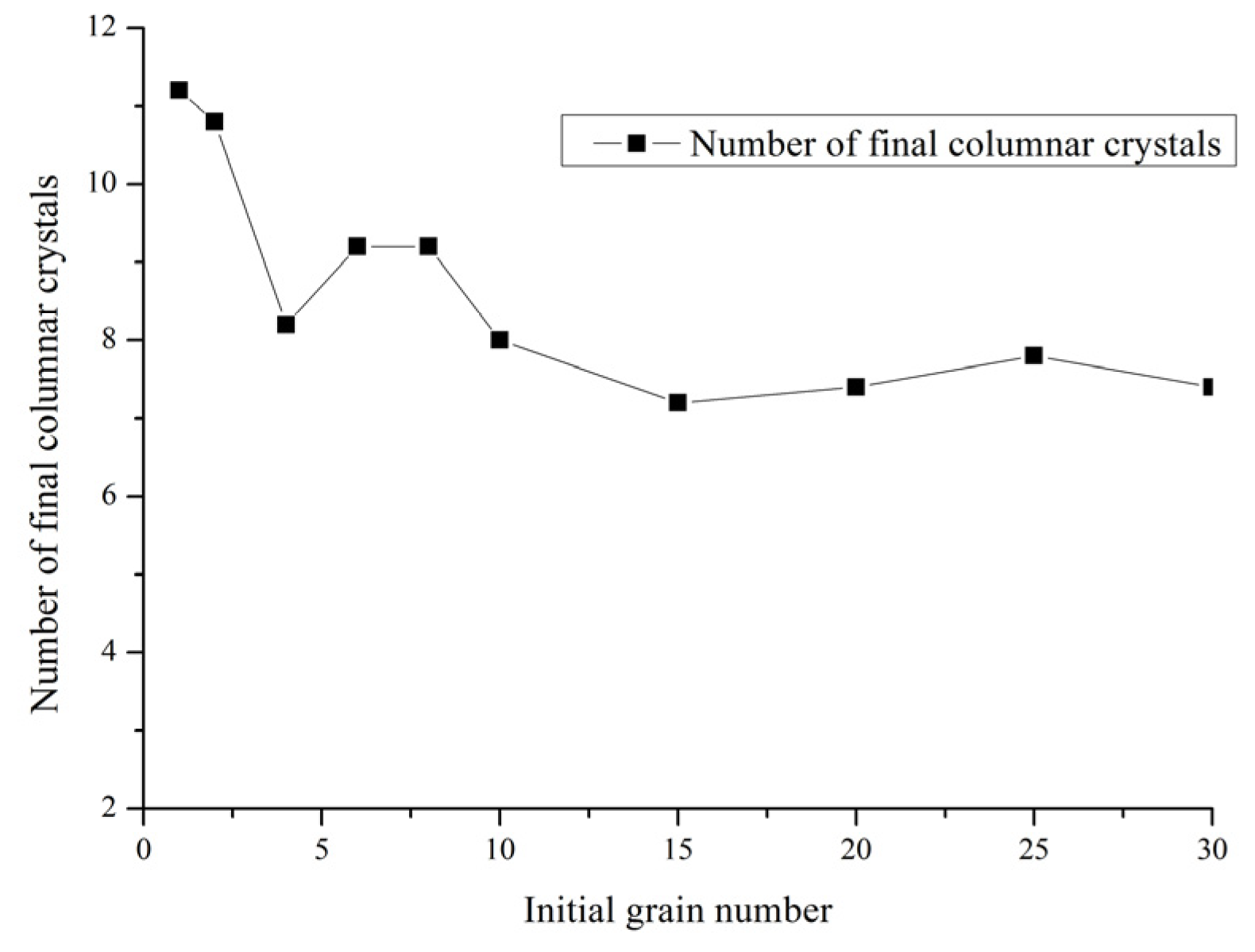
The final number of columnar crystals corresponding to the five calculations of different initial nucleation densities is summarized in

Table 2. Final number of columnar crystals calculated with different initial crystal grains and different randomly chosen initial positions (calculations 1–5).

Number of Equiaxed Grains	Number of Columnar Crystals
	Calculation No. 1	Calculation No. 2	Calculation No. 3	Calculation No. 4	Calculation No. 5	Average Value
1	14	10	14	8	10	11.2
2	10	11	12	11	10	10.8
4	5	8	7	13	8	8.2
6	8	8	9	10	11	9.2
8	10	10	9	8	9	9.2
10	8	8	8	8	8	8.0
15	8	7	7	6	8	7.2
20	7	7	6	8	9	7.4
25	10	6	7	8	8	7.8
30	8	7	6	8	8	7.4

. The final number of columnar crystals in the random calculation results of a different initial number of grains is taken as the average value. The relationship between the fully developed average number of columnar crystals and the initial number of grains is shown in Figure 9.

It can be seen from Table 2 that when the initial number of grains is 1, the number of columnar crystals is the most. This is because the columnar crystals are all developed from the same grain, so the preferred growth angle of each columnar crystal is the same, and the columnar crystals grow in parallel with each other, so there is no competitive growth behavior. When the initial number of grains is 2, there are only two kinds of preferred angles for dendrites, and the number of columnar grains is also larger. When the initial number of grains continues to increase, the number of columnar grains generally decreases. When the initial number of grains exceeds a certain number, the number of columnar grains finally formed tends to a stable value, as shown in Figure 9. This shows that in the actual casting process, the initial equiaxed grain density on the wall has no significant effect on the density of columnar grains finally formed.

4.2. The Effect of Wall Grain Density on Thickness of Equiaxed Layer

The equiaxed grains on the wall first grow freely close to the wall during the solidification process. When they are close to other grains, they will compete with each other, so a layer of equiaxed grains will be formed on the wall. In this section, the effect of the wall grain density on the thickness of the equiaxed crystal layer was studied.

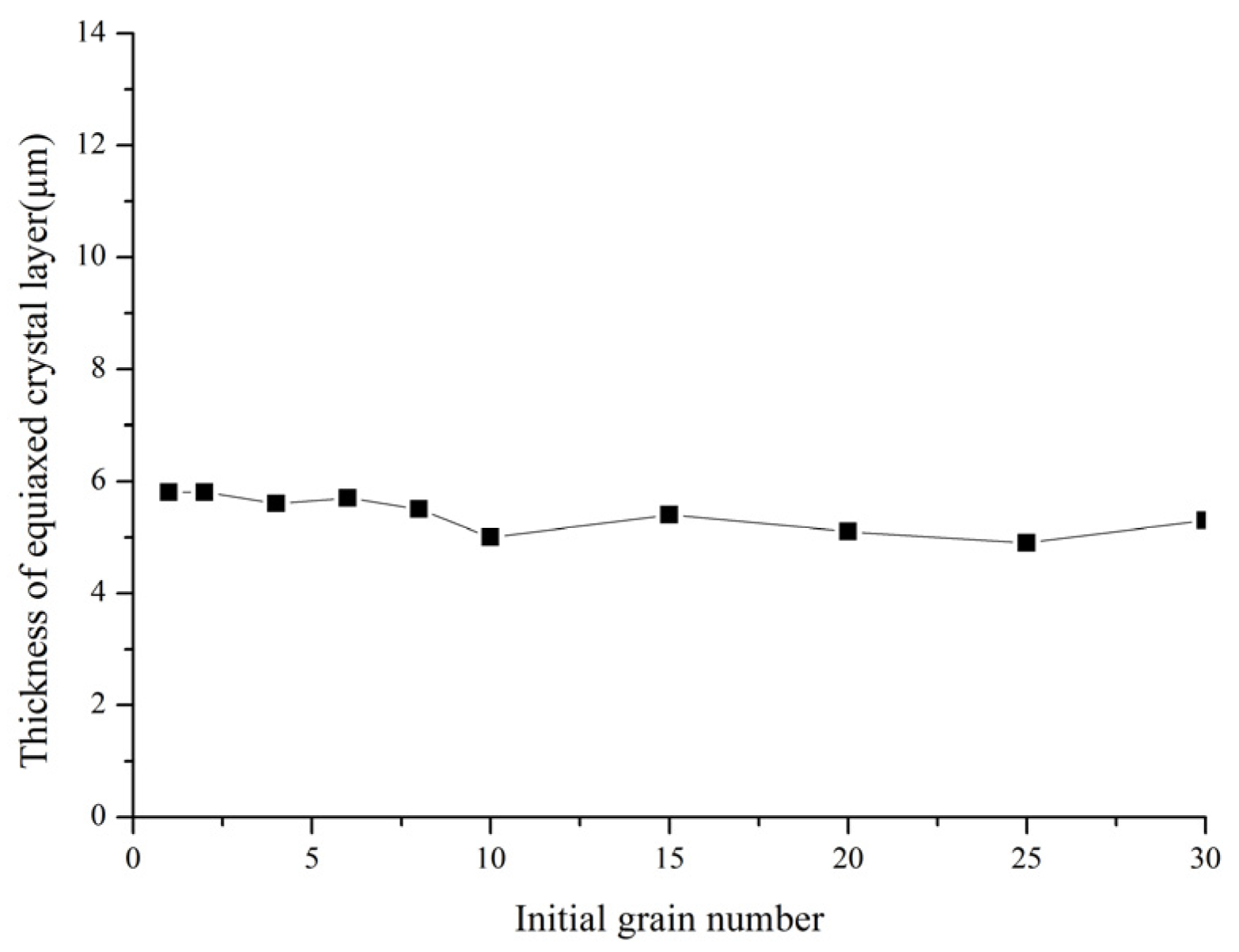
The thickness of the equiaxed crystal layer was calculated by different random nucleation numbers on the wall. The calculation conditions were as before, and the calculation results are shown in

Table 3. Thickness of equiaxed crystal layer calculated with different initial crystal grains and different randomly chosen initial positions (calculations 1–5).

Number of Equiaxed Grains	The Thickness of the Equiaxed Crystal Layer (μm)
	Calculation No. 1	Calculation No. 2	Calculation No. 3	Calculation No. 4	Calculation No. 5	Average Value
1	4.5	6.5	5.0	7.0	6.0	5.8
2	5.0	5.0	6.0	7.0	6.0	5.8
4	6.0	6.0	5.5	5.0	5.5	5.6
6	7.0	5.0	5.5	5.5	5.5	5.7
8	5.5	5.5	5.5	6.0	5.0	5.5
10	5.0	5.0	5.0	5.0	5.0	5.0
15	5.5	6.0	5.0	6.0	4.5	5.4
20	5.0	4.5	5.5	5.0	5.5	5.1
25	4.5	5.0	5.0	5.0	5.0	4.9
30	5.5	5.0	5.5	5.5	5.0	5.3

. The averages of the values in the table have been taken to produce Figure 10.

It can be seen from Table 3 and Figure 10 that the thickness of the equiaxed crystal layer is basically independent of the initial number of equiaxed crystals, and it is always stable at about 5.5 μm. In the case of a certain cooling strength, even for a single crystal grain, the density of the secondary and multiple branches remains constant during the spreading process on the wall surface, so an equiaxed crystal layer with the same thickness as the polycrystalline grain will be formed on the wall surface.

4.3. The Effect of Supercooling Degree and Heat Transfer Coefficient on Cylindrical Crystal Density

In this section, different supercooling degrees and surface heat exchange coefficients were set based on the calculation in the previous sections. The influence of supercooling degree and heat dissipation intensity on the density of columnar crystals was studied by comparing the calculation results in the previous section. First, the influence of the heat exchange coefficient on the density of columnar crystals was calculated. The heat exchange coefficient was set to 1000 W·m⁻² K⁻¹ with the remaining calculation parameters unchanged. Similar to the calculation designed in the previous section, in order to fully reflect the general variation rule of columnar crystal density under different initial grain densities when changing the heat exchange coefficient, 10 different initial grain numbers were calculated. Five calculations were carried out for each initial grain number, and the average number of columnar crystals and the average equiaxed layer thickness corresponding to each initial grain number were calculated.

The final number of columnar crystals corresponding to the five calculations of different initial nucleation densities is summarized in

Table 4. Final number of columnar grains calculated with different initial crystal grains and different randomly chosen initial positions (calculations 1–5) when heat transfer coefficient is 1000 W·m⁻² K⁻¹.

Number of Equiaxed Grains	Number of Columnar Crystals
	Calculation No. 1	Calculation No. 2	Calculation No. 3	Calculation No. 4	Calculation No. 5	Average Value
1	7	9	6	4	5	6.2
2	4	4	6	5	4	4.6
4	6	6	4	7	4	5.4
6	6	4	4	4	6	4.8
8	5	5	6	7	4	5.4
10	4	5	4	6	5	4.8
15	5	6	5	4	6	5.2
20	7	6	6	7	8	6.8
25	4	8	8	6	6	6.4
30	6	5	8	7	7	6.6

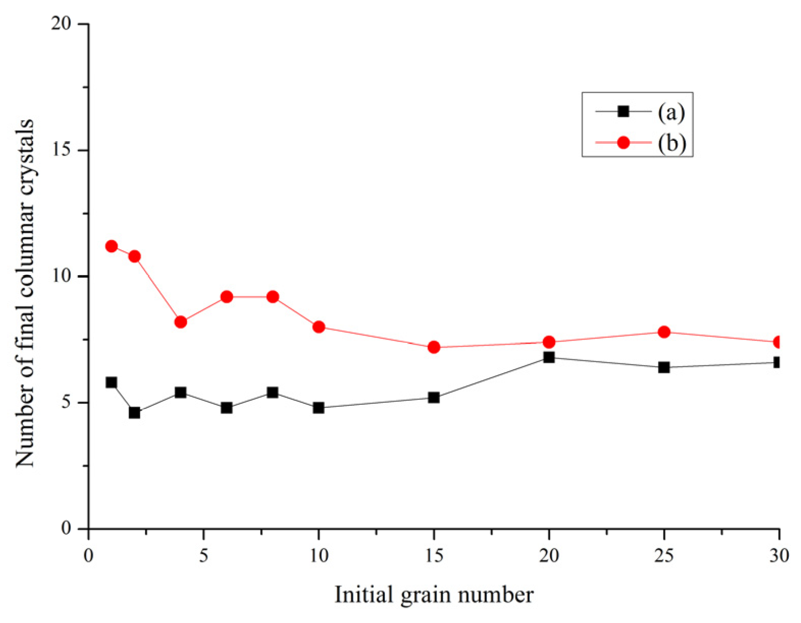
. Figure 11 shows a comparison diagram of the average final columnar crystal numbers corresponding to different initial crystal grain numbers when the heat transfer coefficients are 1000 and 2000 W·m⁻² K⁻¹. From Table 4, it can be seen that the average number of final columnar crystals corresponding to different initial grains has little difference when the heat exchange coefficient is 1000 W·m⁻² K⁻¹. It is shown that the relationship between the number of columnar crystals and initial crystals does not change with the heat transfer coefficient. From Figure 11, it can be seen that when the heat exchange coefficient decreases, the average number of columnar crystals corresponding to different initial grains decreases, i.e., the smaller the cooling intensity on the cooling surface and the smaller the number of columnar crystals, the larger the size of columnar crystals when the solidification is completed, which is consistent with the solidification principle.

The equiaxed crystal layer thickness corresponding to the five calculations of different initial nucleation densities in this group is summarized in

Table 5. Thickness of equiaxed crystal layer calculated with different initial crystal grains and different randomly chosen initial positions (calculations 1–5) with heat transfer coefficient of 1000 W·m⁻² K⁻¹.

Number of Equiaxed Grains	The Thickness of the Equiaxed Crystal Layer (μm)
	Calculation No. 1	Calculation No. 2	Calculation No. 3	Calculation No. 4	Calculation No. 5	Average Value
1	4.5	4.0	4.5	5.5	4.0	4.5
2	4.0	3.5	4.5	3.5	4.0	3.9
4	4.0	4.0	4.0	5.0	4.0	4.2
6	4.0	4.0	4.0	4.0	4.0	4.0
8	4.0	4.0	4.0	4.0	4.0	4.0
10	4.0	4.0	4.0	4.0	4.0	4.0
15	4.0	3.5	4.5	3.5	4.0	3.9
20	4.0	4.5	4.0	4.0	4.0	4.1
25	4.0	4.0	3.5	4.0	4.0	3.9
30	4.0	4.0	3.5	4.0	4.5	4.0

. It can be seen that the average equiaxed crystal layer thickness corresponding to different initial grain numbers is stable at about 4.0, which indicates that the thickness of the equiaxed crystal layer is basically independent of the number of initial equiaxed crystals at different heat exchange coefficients. Figure 12 is a comparison of the average equiaxed crystal layer thickness corresponding to different initial grains with two heat transfer coefficients. It can be seen that when the heat transfer coefficient is reduced, the average equiaxed crystal layer thickness corresponding to different initial grains decreases, i.e., the smaller the cooling intensity on the heat dissipation surface, the smaller the equiaxed crystal thickness. This is because the cooling ability of the cooling surface directly affects the driving force of the competitive growth of grains. The smaller the cooling capacity, the smaller the driving force of grain-oriented growth, and the less intense the competition between dendrites is. Therefore, the more dendrites that can participate in the competitive growth, the fewer grains that cannot participate in the competitive growth, finally decreasing the thickness of the equiaxed crystal layer.

Next, the effect of undercooling on the density of fully developed columnar crystals was calculated. The supercooling of the calculation domain was set to 3 K, and the other calculation parameters remained unchanged. This set of calculations is the same as that in the study of the heat dissipation coefficient. A total of 50 calculations were performed. The final calculation results of the number of columnar crystals and the thickness of the equiaxed crystal layer are summarized in

Table 6. The final number of columnar crystals calculated with different initial crystal grains and different randomly chosen initial positions (calculations 1–5) when the supercooling degree is 3 K.

Number of Equiaxed Grains	Number of Columnar Crystals
	Calculation No. 1	Calculation No. 2	Calculation No. 3	Calculation No. 4	Calculation No. 5	Average Value
1	12	15	11	8	6	10.4
2	14	8	6	10	4	8.4
4	6	7	9	11	4	7.4
6	6	6	7	7	8	6.8
8	9	8	5	7	4	6.6
10	7	7	6	8	7	7.0
15	5	5	8	5	6	5.8
20	6	5	5	6	6	5.6
25	6	7	7	6	7	6.6
30	7	6	7	7	7	6.8

and

Table 7. The thickness of the equiaxed crystal layer calculated with different initial crystal grains and different randomly chosen initial positions (calculations 1–5) when the undercooling degree is 3 K.

Number of Equiaxed Grains	The Thickness of the Equiaxed Crystal Layer (μm)
	Calculation No. 1	Calculation No. 1	Calculation No. 1	Calculation No. 1	Calculation No. 1	Average Value
1	7.0	6.5	7.0	6.5	7.0	6.8
2	5.5	6.0	6.0	6.0	6.5	6.0
4	7.0	5.0	6.5	5.0	6.0	5.9
6	6.5	6.5	5.5	5.5	5.0	5.8
8	5.0	6.0	6.0	5.0	6.0	5.6
10	5.5	6.0	6.0	6.0	5.5	5.8
15	6.5	6.5	5.0	5.0	5.5	5.7
20	5.0	6.0	5.5	5.5	6.5	5.7
25	5.5	6.0	5.5	5.0	6.0	5.6
30	6.0	5.5	5.5	5.0	5.5	5.5

, respectively. Figure 13 and Figure 14 show the comparison between the average number of final columnar crystals and the average thickness of the equiaxed crystal layer when the undercoolings are 3 and 6 K, respectively.

It can be seen from Table 6 that when the undercooling is 3 K, the relationship between the average number of final columnar grains and the initial number of grains still conforms to the previous rule, that is, although the initial number of grains increases continuously, the number of final columnar grains is still relatively stable, and the average number of columnar grains is about 7.4. It can be seen from Figure 13 that when the undercooling is 3 K, the number of fully developed columnar crystals decreases slightly compared with 6 K, so the columnar crystals with a smaller number but larger size will be formed after solidification, which is in line with the solidification principle. It can be seen from Table 7 that when the undercooling is 3 K, the thickness of the equiaxed crystal layer corresponding to different initial grain numbers also has little difference, with an average value of about 5.8, indicating that the thickness of the equiaxed crystal layer is not affected by the initial grain number under different undercoolings. It can be seen from Figure 14 that when the undercooling is 3 K, the thickness of the equiaxed crystal layer is larger than that of 6 K, that is, the thickness of the equiaxed crystal layer will increase with the decrease in undercooling. Unlike the influence of the heat transfer coefficient on the thickness of the equiaxed crystal layer, the decrease in undercooling degree affects the driving force of grain growth. When the undercooling degree changes from 6 to 3 K, the growth velocity of wall grain slows down, and the time for the equiaxed grain to grow to a columnar grain increases, so the equiaxed grain layer becomes thicker.

5. Conclusions

In this paper, a three-dimensional LBM-CA coupling model was established by using two sets of grid methods, and the rationality of the model was verified. This model was used to study the effect of the wall-equiaxed crystal density on the number of columnar crystals and the thickness of the equiaxed crystal layer, and the following conclusions were obtained: (1) Under the same solidification condition, the initial equiaxed crystal density on the wall has no significant effect on the final cylindrical crystal density and the thickness of the equiaxed crystal layer. (2) When the other conditions are the same, the lower the supercooling degree, the smaller the number of fully developed cylindrical crystals and the thicker the equiaxed crystal layer. With the decrease in heat exchange coefficient, the number of cylindrical crystals decreases and the thickness of the equiaxed crystal layer decreases.