Modeling and Reconstruction Strategy for Compton Scattering Tomography with Scintillation Crystals

Abstract

The recent development of energy-resolved scintillation crystals opens the way to build novel imaging concepts based on the variable energy. Among them, Compton scattering tomography (CST) is one of the most ambitious concepts. Akin to Computerized Tomography (CT), it consists in probing the attenuation map of an object of interest using external ionizing sources but strives to exploit the scattered radiation as an imaging agent. For medical applications, the scattered radiation represents 70 to 80% when the energy of the source is larger than 100 keV and results from the Compton effect. This phenomenon stands for the collision of a photon with an electron and rules the change of course and loss of energy undergone by the photon. In this article, we propose a modeling for the scattered radiation assuming polychromatic sources such as 60Co and scintillation crystals such as LBC:Ce. Further, we design a general strategy for reconstructing the electron density of the target specimen. Our results are illustrated for toy objects.

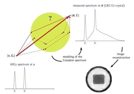
1. Introduction

Invented and theorized by the Nobel medal award-winners G. Houndsfield and A.M. Cormack between 1963 and 1979, the concept of Computerized Tomography (CT) has become an essential way to investigate the inside of a human body or of any type of medium. Its principle relies on the phenomenon of attenuation, characterized by the map ${\mu }_E$, suffered by a photon-beam which travels through matter. This phenomenon is ruled by the Beer–Lambert law

$$\begin{array}{c}\hfill I(\mathbf{x}+T\theta ,\theta ,E)=I(\mathbf{x},\theta ,E)A_E(\mathbf{x},\mathbf{x}+T\theta )=g_0(E,\mathbf{x}+T\theta ,\mathbf{x})\\ \hfill \mathrm{with}{A}_E(\mathbf{x},\mathbf{x}+T\theta )=exp\left(-{\int }_0^T{\mu }_E(\mathbf{x}+t\theta )\mathrm{d}t\right)\end{array}$$

(1)

which quantifies the loss of intensity $I(\mathbf{x},\theta ,E)$ of the photon beam by the exponential of the total attenuation along the travel path between $\mathbf{x}$ and $\mathbf{x}+T\theta$.

For instance, in a fan-beam CT-scan, an X-ray tube illuminates a target with a given intensity. A set of detectors located outside the target, typically on an annulus, will collect the incoming photon flux and characterize the attenuation map of the medium according to the Beer–Lambert law Equation (1). Afterwards, the general (inverse) problem consists in reconstructing the attenuation map ${\mu }_E$ from the measured beam intensities for different angular views. We refer to [1,2] for a general review on reconstruction algorithms for imaging techniques. Since the advent of CT, many imaging concepts have emerged and the need in imaging has grown. One can mention Single Photon Emission CT (SPECT), Positron Emission Tomography (PET) and also Cone-Beam CT for the imaging systems based on an ionizing source.

Due to technological limitations, the factor energy has first been ignored as a potential parameter for an imaging system. However, the development of crystals and detector fabrication technologies enabling the collection of photons and separating them by range of energies has opened the way to many more imaging architectures capable of enhancing the image quality, optimizing the acquisition process or compensating for some limitations (such as limited angle issues), see [3,4,5,6,7,8,9,10]. Furthermore, the use of high-energy X-rays has increased over the years and shows interesting properties for industrial applications, see [11,12,13]. In order to provide a reliable information for an imaging system based on Compton scattering, the crystals should have:

• Good energy resolution;
• High density, high atomic number which enhances the probability for photoelectric absorption;
• No intrinsic activity in the measurement range (355 keV, 1332 keV) which would create a disturbance in the measured distribution;
• Small size and compactness.

In this communication, we will consider the example of LBC:Ce scintillators, which provides a better energy resolution than CeBr₃ scintillators and estimates their impact on our approach. We refer to [14,15] for an exhaustive study on CeBr₃. LBC:Ce scintillation crystals can now be produced with 5 cm diameter, 5cm thickness and achieve about 2.8% FWHM at 662 keV [16,17]. Furthermore, one can note that LBC:Ce is self-radioactive but only in the range from 1550 keV to 2250 keV [18] which is over the measurement range (355 keV, 1332 keV) considered here.

Table 1. Characteristics of LBC:Ce and CeBr₃ crystals.

	LBC:Ce	CeBr3
Emission Wavelength [nm]	380	380
Energy resolution at 662 keV [% FWHM]	2.8	3.8
Light Yield [photons/MeV]	75,000	60,000
Decay Time [ns]	<25	19
Density [g/cm3]	≈5	5.1
Atomic Number (effective)	44 … 45.2	45.9
Intrinsic Activity [Bq/cm3] in range [1550 keV, 2250 keV]	≈1.5	<0.002
hygroscopic	yes	yes

delivers the characteristics of LBC:Ce and CeBr₃ crystals which motivates the use of LBC:Ce crystals for our application, see [17]. Regarding the density of the crystals, we should properly distinguish between crystals and scanning objects. Indeed, both object and crystal will scatter the radiation to some extent. Since this study focuses on the scattering induced by the object, the crystals are assumed to perfectly absorb the scattered radiation.

The physical interactions between photons and matter can be distinguished into: Thomson–Rayleigh scattering, photoelectric absorption, Compton scattering and pair production. In the classic range of applications of the X-rays or $\gamma$-rays, i.e., >60 keV, the photoelectric absorption and the Compton scattering are the dominant phenomena, see [19]. While the photoelectric absorption plays an important role in the attenuation of the photon beam, a measured photon either suffers no interaction (primary radiation) or is scattered (scattered radiation); this is the reason why the Compton scattering is more natural to exploit than the photoelectric effect as an imaging agent.

The Compton effect stands for the collision of a photon with an electron. The photon transfers a part of its energy $E_0$ to the electron which experiences a recoil while the photon is scattered by an (scattering) angle $\omega$ with the axis of propagation, see Figure 1. The energy of the photon after scattering is expressed by the Compton formula [20],

$$E_1=\frac{E_0}{1+\frac{E_0}{m{c}^2}(1-cos\omega )}=\mathcal{E}(E_0,\omega ),$$

(2)

where $m{c}^2=511$ keV represents the energy of an electron at rest.

Usually energy resolved cameras are collimated and combined with polychromatic sources, leading to multi-channel CT-data and corresponding estimations of the attenuation map. Here, we intend to focus instead on the phenomenon of Compton scattering which enables a modeling of the energetic data in terms of electron density and for corresponding emission energies, see [21,22,23,24,25,26,27,28,29,30,31,32,33,34,35,36]. The purpose of this communication is to validate the possibility to use scintillation crystals and their energetic sensitivity in a fan-beam CT scan from a bichromatic ionizing source (here the Cobalt-60). To achieve this, the modeling and the reconstruction strategy are presented in Section 2. Section 3 presents the architecture and properties of the designed scanner with synthetic data as well as reconstructions. The validation of our approach with the properties of the LBC:Ce scintillators motivates the potential of the imaging system in particular with better resolved crystals or semiconductor detectors such as CZT (CdZnTe) [37].

2. Modeling and Processing of the Compton Scattered Data

We first assume the source to be monochromatic, i.e., it emits photons with same energy $E_0$, for the sake of clarity. For sufficiently large $E_0$, larger than 80 keV in medical applications for instance, the Compton effect represents a substantial part of the radiation as more than 70% of the emitted radiation is scattered within the whole body. As depicted by Figure 2, the Compton effect ruled by Equation (2) brings an interesting diversity into the measured spectrum as a monochromatic source leads to a polychromatic radiation measured by scintillation crystals. The development of scintillation crystals such as LBC:Ce and the improvement of their energy resolution delivers a new dimension to explore.

Neglecting Thomson–Rayleigh scattering and the pair production, we focus on the Compton scattering to interpret our data and decompose the spectrum $\mathrm{Spec}(E,\mathbf{s},\mathbf{d})$ measured at a detector $\mathbf{d}$ with energy E as follows

$$\mathrm{Spec}(E,\mathbf{s},\mathbf{d})=\sum _{n=0}^{\infty }{g}_n(E_0,E,\mathbf{s},\mathbf{d}).$$

(3)

In this equation, $g_0$ represents the primary radiation which crossed the object without being subject to the Compton effect. It corresponds to the signal measured in conventional CT, Equation (1). The functions $g_n(E,\mathbf{s},\mathbf{d})$ correspond to the photons that were measured at $\mathbf{d}$ with incoming energy E after n scattering events. The schematic curve with marks ∘ depicted in Figure 2 (right), often called Compton scattered spectrum, is typical from what one observes when measuring the spectrum of a monochromatic source, see for instance [38]. We refer to [39] for a detailed review on the technology of detection.

In the following, we study how the scattered radiation $g_n$, $n=1,2,\dots$ behaves and explain how to deal with it. To simplify the notations, we denote $E_{n+1}=\mathcal{E}(E_n,{\omega }_{n+1})$ with $E_n$ the scattered energy after n scattering events and ${\omega }_{n+1}$ the $(n+1)$th scattering angle.

2.1. The Scattered Flux

We first focus on the first-order scattering as depicted in Figure 1 and Figure 3 for the notations. The travel of a scattered photon beam follows the same scheme:

• The photon beam is emitted by the point source $\mathbf{s}$ in a differential solid angle $\mathrm{d}{\mathsf{\Omega }}_c$ with an energy $E_0$;
• Photons may be absorbed or scattered along the path following the Beer–Lambert law (Equation (1)) leading to the attenuation of the beam by the weight $A_{E_0}(\mathbf{s},\mathbf{x})$;
• A part of the beam may collide with an electron at position ${\mathbf{x}}_1$ which belongs to a differential volume $\mathrm{d}\mathbf{x}$;
• Due to Compton scattering, the photon is scattered by an angle ${\omega }_1$ within a solid angle $\mathrm{d}{\mathsf{\Omega }}_c$ which follows the Klein–Nishina probability ${\left(\frac{d\sigma }{d\mathsf{\Omega }}\right)}_{{\omega }_1}$ ([40]);
• Again the scattered beam is attenuated by a weight $A_{E_1}(\mathbf{x},\mathbf{d})$ due to absorption or scattering of higher order;
• The attenuated and scattered beam finally reaches the point detector at $\mathbf{d}$.

This scheme leads to model the variation of the number of photons $g_1$ scattered at $\mathbf{x}$ and detected at $\mathbf{d}$ with energy $E_1$ by

$$\frac{{\mathrm{d}}^3{g}_1(\mathbf{x},\mathbf{d},\mathbf{s})}{\mathrm{d}\mathbf{x}\mathrm{d}{\mathsf{\Omega }}_c^2}=I(\mathbf{s},\mathbf{x}-\mathbf{s};E_0){\left(\frac{d\sigma }{d\mathsf{\Omega }}\right)}_{{\omega }_1}{A}_{E_0}(\mathbf{s},\mathbf{x})A_{E_1}(\mathbf{x},\mathbf{d})n_e\left(\mathbf{x}\right).$$

(4)

The second variable in the intensity I allows the source to be anisotropic. This formula describes the evolution of the first scattered radiation which is detected at a given energy and at a given detector position.

Regarding the first-order scattering, the Compton Formula (2) relates the energy to the scattering angle and thus delivers a unique geometry for each energy measured. Indeed, all scattering points $\mathbf{x}$ responsible for a detected scattered photon at energy $E_1$ belong to

$$\mathfrak{T}({\omega }_1,\mathbf{s},\mathbf{d})=\left\{\mathbf{x}\in {\mathbb{R}}^3:\frac{\mathbf{x}-\mathbf{s}}{\parallel \mathbf{x}-\mathbf{s}\parallel }·\frac{\mathbf{d}-\mathbf{x}}{\parallel \mathbf{d}-\mathbf{x}\parallel }=cos{\omega }_1\right\}.$$

(5)

$\mathfrak{T}({\omega }_1,\mathbf{s},\mathbf{d})$ defines in 3D the lemon part of a spindle torus (${\omega }_1<\pi /2$) and the apple part of a spindle torus (${\omega }_1>\pi /2$). In 2D, this reduces to two circular-arcs as depicted in Figure 4a. Figure 4b shows the scanning of a specimen by paired circular-arcs for different energy levels or equivalently different scattering angles ${\omega }_1$.

An integral modeling of $g_1$ can then be obtained by integrating Equation (4) over the whole domain of the specimen and leads to a generalized Radon transform along $\mathfrak{T}({\omega }_1,\mathbf{s},\mathbf{d})$, noted ${\mathcal{C}}_1\left(n_e\right)$,

$${\mathcal{C}}_1\left(n_e\right)(E_0,E_1,\mathbf{s},\mathbf{d})={\int }_{\mathfrak{T}({\omega }_1,\mathbf{s},\mathbf{d})}I(\mathbf{s},\mathbf{x}-\mathbf{s};E_0){\left(\frac{d\sigma }{d\mathsf{\Omega }}\right)}_{{\omega }_1}{A}_{E_0}(\mathbf{s},\mathbf{x})A_{E_1}(\mathbf{x},\mathbf{d})n_e\left(\mathbf{x}\right)\mathrm{d}\mathbf{x}.$$

(6)

We refer to [41,42] for more details.

As explained above, the spectrum cannot be reduced to the first-order scattering and multiple scattering must be taken into account. However, the question of its modeling arises. Physically, the same reasoning as for the first-order scattering can be iterated. The second-order scattering is illustrated in Figure 3. The computation of the successive scattering events leads thus to

$$\frac{{\mathrm{d}}^{2n+1}{g}_n({\mathbf{x}}_0,\dots ,{\mathbf{x}}_{n+1})}{\mathrm{d}{\mathbf{x}}_1\dots \mathrm{d}{\mathbf{x}}_n\mathrm{d}{\mathsf{\Omega }}_c^{n+1}}=I({\mathbf{x}}_0,{\mathbf{x}}_1-{\mathbf{x}}_0;E_0)\prod _{i=1}^n{\left(\frac{d\sigma }{d\mathsf{\Omega }}\right)}_{{\omega }_i}{A}_{E_{i-1}}({\mathbf{x}}_{i-1},{\mathbf{x}}_i)A_{E_i}({\mathbf{x}}_i,{\mathbf{x}}_{i+1})n_e\left({\mathbf{x}}_i\right),$$

(7)

with ${\mathbf{x}}_0=\mathbf{s}$ and ${\mathbf{x}}_{n+1}=\mathbf{d}$. The components of the spectral data are then the functions $g_n$ obtained by integrating Equation (7) over the support of the object. The difficulty here is the interpretation of this variation as an operator ${\mathcal{C}}_n\left(n_e\right)$ due to the complicated relations between successive scattering angles and the measured energy. This work was done for $n=2$ in [41] for the 3D case and in [42] for the 2D case. The model is similar to ${\mathcal{C}}_1$ but with a trickier integration support and a quadratic dependency on the electron density.

2.2. Extension to Polychromatic $\gamma$-ray Sources

Monochromatic sources are of course difficult to produce and extremely expensive. While X-ray tubes produce a wide spectrum with few characteristic peaks, $\gamma$-ray sources emit essentially photons with energies at their characteristic peaks. In both cases, the spectrum of an ionizing source can be decomposed into

$$T\left(E\right)=T_{flat}\left(E\right)+\sum _{i=1}^N{T}_{peak}^{\left(i\right)}\left(E\right)$$

(8)

with $T_{flat}$ the smooth and wide part of the spectrum and $T_{peak}^{\left(i\right)}$ the characteristic peaks. Including this information into the scattered spectrum in Equation (3) leads to

$${\mathrm{Spec}}_T(E,\mathbf{s},\mathbf{d})=\sum _{n=0}^{\infty }{\int }_0^{\infty }T\left(E_0\right)g_n(E_0,E,\mathbf{s},\mathbf{d})\mathrm{d}{E}_0.$$

(9)

In this work, we consider the widely used Cobalt-60 which produces two characteristic peaks at $E_0^{\left(1\right)}=1.173$ MeV and $E_0^{\left(2\right)}=1.333$ MeV. In that case, one can interpret the measured spectral data after scattering by

$${\mathrm{Spec}}_{C{o}^{60}}(E,\mathbf{s},\mathbf{d})=\sum _{n=0}^{\infty }{\mathcal{C}}_n\left(n_e\right)(E_0^{\left(1\right)},E,\mathbf{s},\mathbf{d})+{\mathcal{C}}_n\left(n_e\right)(E_0^{\left(2\right)},E,\mathbf{s},\mathbf{d})$$

(10)

using the integral modeling for $g_n$.

2.3. Modeling the Impact of the Scintillation Crystals

For 60Co sources, LBC:Ce crystals demonstrates a 2.8% FWHM at 662 keV, 2.1% FWHM at 1.173 MeV and 2% FWHM at 1.332 MeV. This resolution as well as its diameter 5cm has a huge impact on our modeling and on the quality of the scattered data. Since an exact estimation of the point spread function in our model is extremely difficult due to the complexity of scattering inside the crystals, it can be relevant to simplify this model to a convolution, noted *, with a Gaussian normal distribution

$$G_{\sigma }\left(E\right)=\frac{1}{\sqrt{2\pi {\sigma }^2}}exp\left(\frac{-{\left|E\right|}^2}{2{\sigma }^2}\right)$$

(11)

with standard deviation satisfying for LBC:Ce crystals

$$\frac{\sigma }{\mathrm{keV}}=0.306\sqrt{\frac{E}{\mathrm{keV}}}.$$

(12)

In addition, the size, shape and potential capsule of the crystal, noted here $\mathbf{Cr}\left(\mathbf{d}\right)$, can have an important impact on the resolution and the measurement, see Figure 5. Indeed, our models ${\mathcal{C}}_n$ assume the crystal to be a point while $\mathbf{Cr}\left(\mathbf{d}\right)$ is in practice a cylinder. Assuming that each element of a crystal behaves as a detector point, our models can thus be adapted by considering the transformation

$$\mathcal{D}g(E,\mathbf{s},\mathbf{d})={\int }_{{\mathbf{d}}^{\prime }\in \mathbf{Cr}\left(\mathbf{d}\right)}g(E,{\mathbf{d}}^{\prime },\mathbf{s})\mathrm{d}{\mathbf{d}}^{\prime }.$$

(13)

We note that depending on the shape of the specimen under study and on the desired resolution of the reconstructed image, the operator $\mathcal{D}$ can be negligible in comparison with the limitations of the energy resolution and the convolution with $G_{\sigma }$. We note also that the thickness of scanning depicted in Figure 5, which affects the final resolution of the reconstructed image, corresponds to between a half and a third of the crystal depth. This is the reason why its impact may be negligible if the achieved image resolution is slightly smaller than the crystal size. This consideration shall be studied more in detail in further studies. Taking into account the stochastic nature of the emission of photons, we obtain a final model

$${\mathrm{Spec}}_{C{o}^{60}}^{LBC}(E,\mathbf{s},\mathbf{d})=\mathrm{Pois}\left(\mathcal{D}{\mathrm{Spec}}_{C{o}^{60}}(·,\mathbf{s},\mathbf{d})\ast G_{\sigma }\right)(E,\mathbf{s},\mathbf{d})$$

(14)

in which $\mathrm{Pois}(·)$ stands for the Poisson distribution and with ${\mathrm{Spec}}_{C{o}^{60}}$ given in Equation (10).

2.4. A General Approach for the Reconstruction of the Electron Density

In order to exploit the scattered spectrum as an imaging agent, we need to find $n_e$ from ${\mathrm{Spec}}_{C{o}^{60}}^{LBC}$ in Equation (14).

The main issue for solving this inverse problem is the complexity of ${\mathcal{C}}_n$, $n>1$, in terms of modelling and computation time. The use of neural networks could circumvent this complexity but the lack of database for such scattered data prevents this approach. The use of standard optimization techniques such as the ROF model for total-variation regularization [43] requires however an accurate knowledge and an efficient computation of the forward model. The only suitable model for such standard approaches in our case is the first-order scattered radiation modelling, ${\mathcal{C}}_1\left(n_e\right)$.

Following on from [41,42], the first-order scattered intensity ${\mathcal{C}}_1\left(n_e\right)$ is less smooth than the multiple-order scattered intensity ${\mathcal{C}}_n\left(n_e\right)$, $n\ge 2$. Indeed, the complexity of multiple scattering tends to smooth the information about the electron density $n_e$ and thus the first-order scattering constitutes the most reliable information in the Compton spectrum. Relying upon theoretical results, this observation implies enhancing the variations of the data in order to reduce the part of multiple scattering. This can be done by considering the following problem:

$$\mathrm{find}{n}_e\mathrm{from}{\partial }_E{\mathrm{Spec}}_{C{o}^{60}}^{LBC}\approx {\partial }_E{\mathcal{C}}_1\left(n_e\right)$$

(15)

in which ${\partial }_E$ denotes the derivative with respect to the energy. Following the ROF-model [43], a solution can be constructed by solving the minimization problem

$$\underset{n_e}{min}\frac{1}{2}{∥{\partial }_E{\mathrm{Spec}}_{C{o}^{60}}^{LBC}-{\partial }_E{\mathcal{C}}_1\left(n_e\right)∥}^2+\lambda TV\left(n_e\right)$$

(16)

where $TV\left(n_e\right)$ stands for the total-variation of $n_e$. We consider this reconstruction method in the following section.

3. A CT-CST Scanner

We propose combining the standard fan-beam CT scanner with CST, see Figure 6. The architecture is identical with the exception that an X-ray tube and the CCD cameras are replaced respectively by a $\gamma$-ray source (60Co) and scintillation crystals (LBC:Ce). Taking advantage of the energetical variable brought by scintillators, we measure only 12 projections. Each projection is obtained by a 30° rotation of the scanner or of the specimen.

In our setting, 40 crystals are placed on the half circle opposite the source position. For simplification of the mathematical and numerical model, every detector as well as the source is modeled as a point of no space expansion. The imaged area is a square centered in the architecture of size $150\times 150{\mathrm{cm}}^2$, see Figure 6a. The complete scanning process is depicted in Figure 6b. Furthermore, the source emits ${10}^6$ photons per projection.

We assume that the energy of the photons is measured in the energy range $[355\mathrm{keV},$$1332\mathrm{keV}]$. The lower bound is hereby chosen as the energy of a photon that has initial energy $1173\mathrm{keV}$ and is scattered once, changing its trajectory angle by $\pi /2$, see Equation (2). The energy range is sampled equidistantly with 128 measured levels, leading to a necessary sampling of $7.68\mathrm{keV}$. In practice, the energy resolution of scintillation crystals is not constant; however, this information can be simply incorporated in our approach and thus we consider a constant energy resolution for the sake of simplicity.

3.1. Ballistic Data

For the simulations, we consider a simple toy object made of an annulus of aluminum with a rectangle of polyethylene inside, see Figure 7a. The details are given in the following

Table 2. Material and dimensions of the specimen and of the scintillator.

	Annulus	Rectangle	Crystal
	Aluminium	Polyethylene	LBC:Ce
Surface	53 cm outer/45 cm inner radius	$45\times 38{\mathrm{cm}}^2$	$5\times 5{\mathrm{cm}}^2$
Thickness	2 cm	2 cm	5 cm

:

The ballistic part of the spectral data, $g_0$ defined in Equation (1), corresponds to the standard measure in CT. Due to the scintillation crystals, the primary measurement suffers also the energy resolution of the LBC:Ce and thus can be modeled by $G_{\sigma }\ast g_0$.

Obtained by the standard TV regularization method [43], the average of the reconstructions of the attenuation map ${\mu }_E$ at energies 1173 and 1333 keV is depicted in Figure 7b. The reconstruction suffers many artifacts which can be explained by: the energy resolution of the crystals and the very limited number of data (12 views and 40 detectors). However, this provides very important information for us. Indeed, at the energy range considered here, $[355\mathrm{keV},$$1332\mathrm{keV}]$, the attenuation map is essentially proportional to the electron density, see [19],

$${\mu }_E\left(\mathbf{x}\right)\approx {\sigma }_c\left(E\right)n_e\left(\mathbf{x}\right)$$

(17)

in which ${\sigma }_c\left(E\right)$ stands for the Compton total-cross section at energy E. Thereby, the ballistic data $g_0$ delivers us a first approximation for the sought-for electron density and can help us to compute a more accurate model ${\mathcal{C}}_1\left(n_e\right)$.

3.2. Results Based on the Compton Scattered Spectrum

Due to the nature of scattering, the complete architecture has to be three dimensional. As an illustration for our general approach, we considered the much simpler fan-beam geometry CT-scan with a 2 cm thickness. This way the geometry of 3D-scattering can be approximated by a 2D-geometry. Therefore, the torus $\mathfrak{T}$, see Equation (5), simplifies to two circular-arcs in this setting.

The scattered data for one projection view is depicted in Figure 8c. The spectrum is here essentially composed of the first-order and second-order scattered radiation, Figure 8a,b, respectively.

In order to emphasize the general reconstruction strategy described in Section 2.4, we consider the profiles of the measured spectrum in Figure 8 for four different detector positions ${\mathbf{d}}_1,{\mathbf{d}}_2,{\mathbf{d}}_3,{\mathbf{d}}_4$ making an angle between source and center of the circle of −20, −10, 0 and 10 degrees respectively. We observe the two characteristic peaks of 60Co and the Compton spectrum composed of first-order and multiple scattering. As demonstrated in [41,42], it is possible to exploit the smoothness properties of the different components of the spectrum. This is done simply by a discrete derivative applied on the spectral data. The derivative of the spectrum for one view and one detector is given in Figure 9. We observe that the differentiation step leads to reducing the part of multiple scattering and highlights the first-order scattering, which has the most suited structure for standard reconstruction methods. Using standard TV-regularization as for the ballistic data, we propose solving the problem (15). The result is depicted in Figure 10b. The reconstruction is satisfactory but has a relative poor accuracy. While the modeling of the crystals has a huge impact on this reconstruction, a more theoretical aspect has to be considered. Indeed, the attenuation factors $A_{E_0}$ and $A_{E_1}$ are the most harmful physical factors of the inverse problem as they increase dramatically the ill-posedness or ill-conditioning of the method, i.e., its instability. While this instability is controlled by the TV-regularization, it leads to a reduced quality of reconstruction. To illustrate this aspect, we consider also reducing the complete system scanner/specimen by a factor of 66%, 50% and 40%. The results are depicted in Figure 10b–d. By downsizing the object, we shorten the length of the photon travel and thus diminish the attenuation weights. As measured by the errors in

Table 3. Peak signal-to-noise ratio and mean square errors of the reconstructions in Figure 10.

	150 cm	100 cm	75 cm	60 cm
PSNR	13.69 dB	18.02 dB	19.16 dB	19.62 dB
MSE	4.28%	1.58%	1.21%	1.09%

, the reconstruction quality increases significantly when we reduce the size of the object. However, it also implies that the crystal size is reduced by the same factor.

4. Conclusions and Discussion

This work illustrates the potential of scintillation crystals in the novel Compton scattering tomography. The Compton spectrum is decomposed into multiple scattering events of order n and modeled by integral transforms. The proposed reconstruction method takes advantage of the smoothness properties of the nth-order scattered radiation by applying standard techniques combined with a differentiation step. As revealed by the simulations, the ill-posedness induced by the attenuation factors and the energy resolution of the crystals has a substantial impact on the quality and accuracy of reconstructions. To address this issue, the development of more flexible and suited reconstruction methods is the core of our future research.

A limitation of this study is the 2D aspect of the simulations. Indeed, the nature of Compton scattering is three dimensional; this is why the simulations made here will be extended to the 3D case in order to reveal the full potential of the approach. In addition, we considered that ≈${10}^7$ photons were emitted by the $\gamma$-ray source for the total of views and were held into the slice of thickness 2 cm. In a real system, many more photons would be required in order to obtain a signal-to-noise ratio satisfactory in the data.

Furthermore, while the reconstruction of the electron density is shown possible, the resolution of reconstruction depends proportionally on the crystal size. Therefore, based on this preliminary work, the relevance and reliability of CST scanners lies upon many technological challenges: (i) the production of scintillation crystals smaller than the millimeter in order to compete with conventional CT, (ii) with the smallest FWHM possible and (iii) the production of $\gamma$-ray sources able to emit a large number of photons (${10}^7$ photons per second) would help the method produce fast and accurate images.

References

- Natterer, F. The Mathematics of Computerized Tomography; Classics in Mathematics; Society for Industrial and Applied Mathematics: New York, NY, USA, 2001. [Google Scholar]
- Natterer, F.; Wübbeling, F. Mathematical Methods in Image Reconstruction; Classics in Mathematics; Society for Industrial and Applied Mathematics: New York, NY, USA, 2001. [Google Scholar]
- Hounsfield, G. Computerized transverse axial scanning (tomography). I. Description of system. Br. J. Radiol. 1973, 46, 1016–1022. [Google Scholar] [CrossRef] [PubMed]
- Alvarez, R.; Macovski, A. Energy-selective reconstructions in X-ray computerized tomography. Phys. Med. Biol. 1976, 21, 733–744. [Google Scholar] [CrossRef]
- Primak, A.; Giraldo, J.R.; Liu, X.; Yu, L.; McCollough, C. Improved dual-energy material discrimination for dual-source CT by means of additional spectral filtration. Med. Phys. 2009, 36, 1359–1369. [Google Scholar] [CrossRef] [Green Version]
- Shefer, E.; Altman, A.; Behling, R.; Goshen, R.; Gregorian, L.; Roterman, Y.; Uman, I.; Wainer, N.; Yagil, Y.; Zarchin, O. State of the Art of CT Detectors and Sources: A Literature Review. Curr. Radiol. Rep. 2013, 1, 76–91. [Google Scholar] [CrossRef]
- Tracey, B.; Miller, E. Stabilizing dual-energy X-ray computed tomography reconstructions using patch-based regularization. Inverse Probl. 2015, 31, 05004. [Google Scholar] [CrossRef] [Green Version]
- McCollough, C.; Leng, S.; Lifeng, Y.; Fletcher, J. Dual- and Multi-Energy CT: Principles, Technical Approaches, and Clinical Applications. Radiology 2015, 276, 637–653. [Google Scholar] [CrossRef] [PubMed]
- Goo, H.; Goo, J. Dual-Energy CT: New Horizon in Medical Imaging. Korean J. Radiol. 2017, 18, 555–569. [Google Scholar] [CrossRef] [Green Version]
- Fredenberg, E. Spectral and dual-energy X-ray imaging for medical applications. Nucl. Instrum. Methods Phys. Res. Sect. A Accel. Spectrometers Detect. Assoc. Equip. 2018, 878, 74–87. [Google Scholar] [CrossRef]
- Tian, Y.; Shimazoe, K.; Yan, X.; Ueda, O.; Ishikura, T.; Fujiwara, T.; Uesaka, M.; Ohno, M.; Tomita, H.; Yoshihara, Y.; et al. High energy X-ray photon counting imaging using linear accelerator and silicon strip detectors. Nucl. Instrum. Methods Phys. Res. Sect. A Accel. Spectrometers Detect. Assoc. Equip. 2016, 830, 251–255. [Google Scholar] [CrossRef]
- Izumi, S.; Kamata, S.; Satoh, K.; Miyai, H. High energy X-ray computed tomography for industrial applications. IEEE Trans. Nucl. Sci. 1993, 40, 158–161. [Google Scholar] [CrossRef]
- Toyokawa, H.; Kanada, H.; Kaihori, T.; Koike, M.; Yamada, K. Application of high-energy photon CT system with laser-Compton scattering to non-destructive test. IEEE Trans. Nucl. Sci. 2008, 55, 3571–3578. [Google Scholar] [CrossRef]
- Fraile, L.M.; Mach, H.; Vedia, V.; Olaizola, B.; Paziy, V.; Picado, E.; Udías, J.M. Fast timing study of a CeBr3 crystal: Time resolution below 120 ps at 60Co energies. Nucl. Instrum. Methods Phys. Res. Sect. A Accel. Spectrometers Detect. Assoc. Equip. 2013, 701, 235–242. [Google Scholar] [CrossRef]
- Otaka, Y.; Shimazoe, K.; Mitsuya, Y.; Uenomachi, M.; Seng, F.W.; Kamada, K.; Yoshikawa, A.; Sakuragi, S.; Binder, T.; Takahashi, H. Performance Evaluation of Liquinert-Processed CeBr3 Crystals Coupled With a Multipixel Photon Counter. IEEE Trans. Nucl. Sci. 2020, 67, 988–993. [Google Scholar] [CrossRef]
- Quarati, F.; Dorenbos, P.; van der Biezen, J.; Owens, A.; Selle, M.; Parthier, L.; Schotanus, P. Scintillation and detection characteristics of high-sensitivity CeBr 3 gamma-ray spectrometers. Nucl. Instrum. Methods Phys. Res. A 2013, 729, 596–604. [Google Scholar] [CrossRef]
- Hellma Materials GmbH. Radiation Detection Crystals. 2014. Available online: https://www.hellma.com/en/crystalline-materials/radiation-detection-crystals/ (accessed on 26 May 2021).
- Hellma Materials GmbH, Scionix Holland BV and Gonitec. Scintillation Properties of High-Resolution La(BrxCl1-x)3:Ce and High-Sensitivity CeBr3. 2017. Available online: https://indico.cern.ch/event/388511/contributions/2612029/attachments/1522152/2378455/SCINT2017_211_Poster.pdf (accessed on 26 May 2021).
- Stonestrom, J.P.; Alvarez, R.E.; Macovski, A. A framework for spectral artifact corrections in X-ray CT. IEEE Trans. Biomed. Eng. 1981, 28, 128–141. [Google Scholar] [CrossRef]
- Compton, A.H. A quantum theory of the scattering of X-rays by light elements. Phys. Rev. 1923, 21, 483–502. [Google Scholar] [CrossRef]
- Lale, P.G. The Examination of Internal Tissues, using Gamma-ray Scatter with a Possible Extension to Megavoltage Radiography. Phys. Med. Biol. 1959, 4, 159–167. [Google Scholar] [CrossRef]
- Norton, S.J. Compton scattering tomography. J. Appl. Phys. 1994, 76, 2007–2015. [Google Scholar] [CrossRef]
- Cesareo, R.; Borlino, C.C.; Brunetti, A.; Golosio, B.; Castellano, A. A simple scanner for Compton tomography. Nucl. Instrum. Methods Phys. Res. A 2002, 487, 188–192. [Google Scholar] [CrossRef]
- Adejumo, O.O.; Balogun, F.A.; Egbedokun, G.G.O. Developing a Compton scattering tomography system for soil studies: Theory. J. Sustain. Dev. Environ. Prot. 2011, 1, 73–81. [Google Scholar]
- Anghaie, S.; Humphries, L.L.; Diaz, N.J. Material characterization and flaw detection, sizing, and location by the differential gamma scattering spectroscopy technique. Part1: Development of theoretical basis. Nucl. Technol. 1990, 91, 361–375. [Google Scholar] [CrossRef]
- Balogun, F.A.; Cruvinel, P.E. Compton scattering tomography in soil compaction study. Nucl. Instrum. Methods Phys. Res. A 2003, 505, 502–507. [Google Scholar] [CrossRef]
- Brunetti, A.; Cesareo, R.; Golosio, B.; Luciano, P.; Ruggero, A. Cork quality estimation by using Compton tomography. Nucl. Instrum. Methods Phys. Res. B 2002, 196, 161–168. [Google Scholar] [CrossRef]
- Clarke, R.L.; Dyk, G.V. A new method for measurement of bone mineral content using both transmitted and scattered beams of gamma-rays. Phys. Med. Biol. 1973, 18, 532–539. [Google Scholar] [CrossRef] [PubMed]
- Evans, B.L.; Martin, J.B.; Burggraf, L.W.; Roggemann, M.C. Nondestructive inspection using Compton scatter tomography. IEEE Trans. Nucl. Sci. 1998, 45, 950–956. [Google Scholar] [CrossRef]
- Farmer, F.T.; Collins, M.P. A new approach to the determination of anatomical cross-sections of the body by Compton scattering of gamma-rays. Phys. Med. Biol. 1971, 16, 577–586. [Google Scholar] [CrossRef]
- Gorshkov, V.A.; Kroening, M.; Anosov, Y.V.; Dorjgochoo, O. X-ray scattering tomography. Nondestruct. Test. Eval. 2005, 20, 147–157. [Google Scholar] [CrossRef]
- Harding, G.; Harding, E. Compton scatter imaging: A tool for historical exploitation. Appl. Radiat. Isot. 2010, 68, 993–1005. [Google Scholar] [CrossRef] [PubMed]
- Meneley, D.A.; Hussein, E.M.A.; Banerjee, S. On the solution of the inverse problem of radiation scattering imaging. Nucl. Sci. Eng. 1986, 92, 341–349. [Google Scholar]
- Arendtsz, N.V.; Hussein, E.M.A. Energy-spectral Compton scatter Imaging—Part 1: Theory and mathematics. IEEE Trans. Nucl. Sci. 1995, 42, 2155–2165. [Google Scholar] [CrossRef]
- Guzzardi, R.; Licitra, G. A critical review of Compton imaging. CRC Crit. Rev. Biomed. Imaging 1988, 15, 237–268. [Google Scholar]
- Rigaud, G. Compton Scattering Tomography: Feature Reconstruction and Rotation-Free Modality. SIAM J. Imaging Sci. 2017, 10, 2217–2249. [Google Scholar] [CrossRef]
- Gurov, Y.B.; Egorov, N.Y.; Ponomarev, D.V.; Rozov, S.V.; Sandukovsky, V.G.; Shakhov, K.V.; Yakushev, E.A.; Zhivun, V.M. Study of characteristics of CdZnTe detector. J. Instrum. 2019, 14, P11002. [Google Scholar] [CrossRef]
- Negm, H.; Ohgaki, H.; Izuru, D.; Hayakawa, T.; Zen, H.; Kii, T.; Masuda, K.; Hori, T.; Hajima, R.; Shizuma, T.; et al. Reaction-yield dependence of the (γ, γ’) reaction of 238U on the target thickness. J. Nucl. Sci. Technol. 2014, 1–10. [Google Scholar] [CrossRef] [Green Version]
- Knoll, G.F. Radiation Detection and Measurement; John Wiley & Sons, Inc.: New York, NY, USA, 1989. [Google Scholar]
- Klein, O.; Nishina, Y. Über die Streuung von Strahlung durch freie Elektronen nach der neuen relativistischen Quantendynamik von Dirac. Z. Phys. 1929, 52, 853–869. [Google Scholar] [CrossRef]
- Rigaud, G. 3D Compton scattering imaging with multiple scattering: Analysis by FIO and contour reconstruction. Inverse Probl. 2021. [Google Scholar] [CrossRef]
- Kuger, L.; Rigaud, G. Joint fan-beam CT and Compton scattering tomography: Analysis and image reconstruction. arXiv 2020, arXiv:2008.06699. [Google Scholar]
- Rudin, L.; Osher, S.; Fatemi, E. Nonlinear total variation based noise removal algorithms. Physica D 1992, 46, 259–268. [Google Scholar] [CrossRef]