The Convolutional Multiple Whole Profile (CMWP) Fitting Method, a Global Optimization Procedure for Microstructure Determination


Abstract
:1. Introduction
2. Fundamental Principles of the Convolutional Multiple-Whole-Profile (CMWP) Optimization Procedure
2.1. Physical and Secondary Parameters in the CMWP Procedure
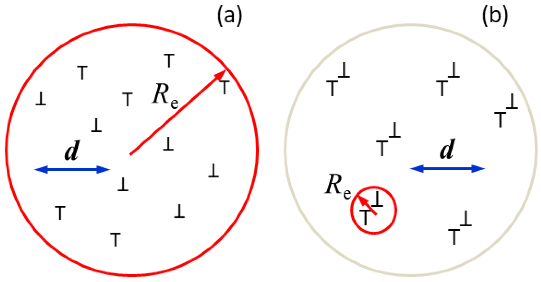
2.1.1. The Density and the Arrangement Parameter of Dislocations
2.1.2. The Contrast Factor of Dislocations
2.1.3. Determination of Slip Modes in hcp Crystals
2.2. Algorithms Used for Solving Equation (7)
2.3. Organization of the Combined LM and MC Algorithms
2.4. Systematic Comparison of the Performance of the LM and MC Procedures
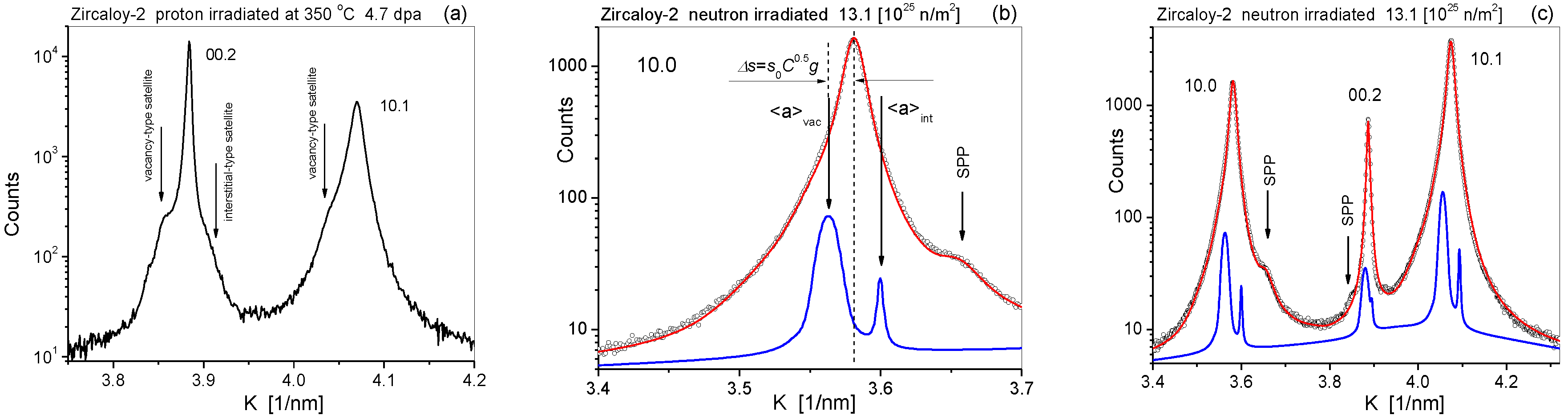
2.5. Extension of CMWP for Handling Satellites or Diffuse Scattering
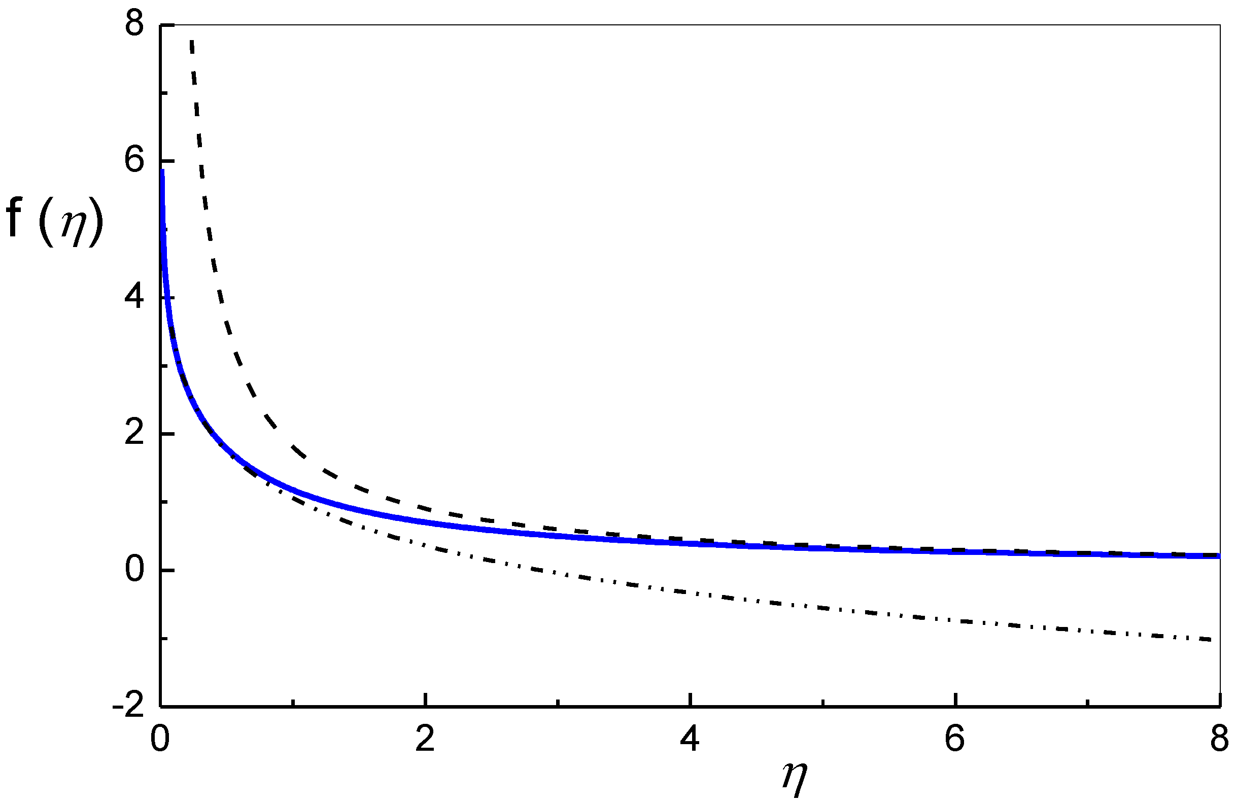
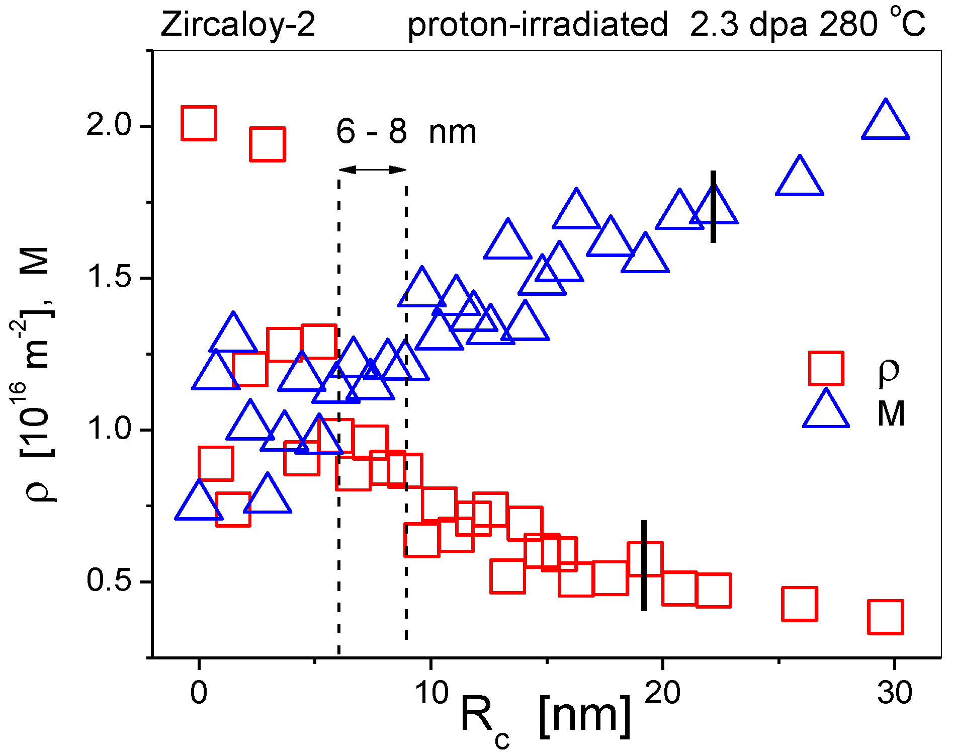
2.6. Stabilizing the Fluctuations of the Physical Parameters When the Effective Outer Cut-Off Radius, Re, Approaches the Lower Limit of Continuum Theory
3. Dislocation Density and Crystallite Size in Zr Matrix and Zr Hydrides in a Hydrated Zircaloy-4 Sheet Material
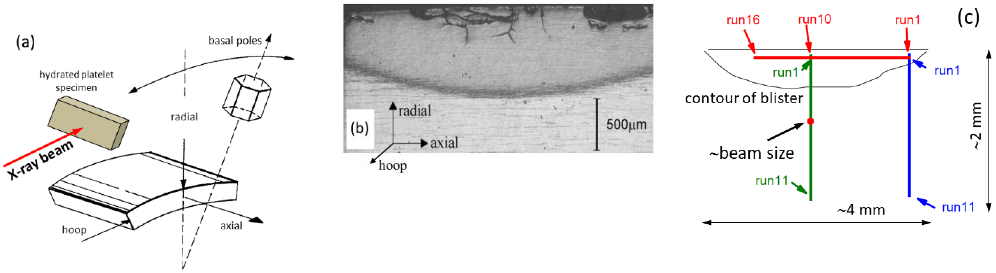
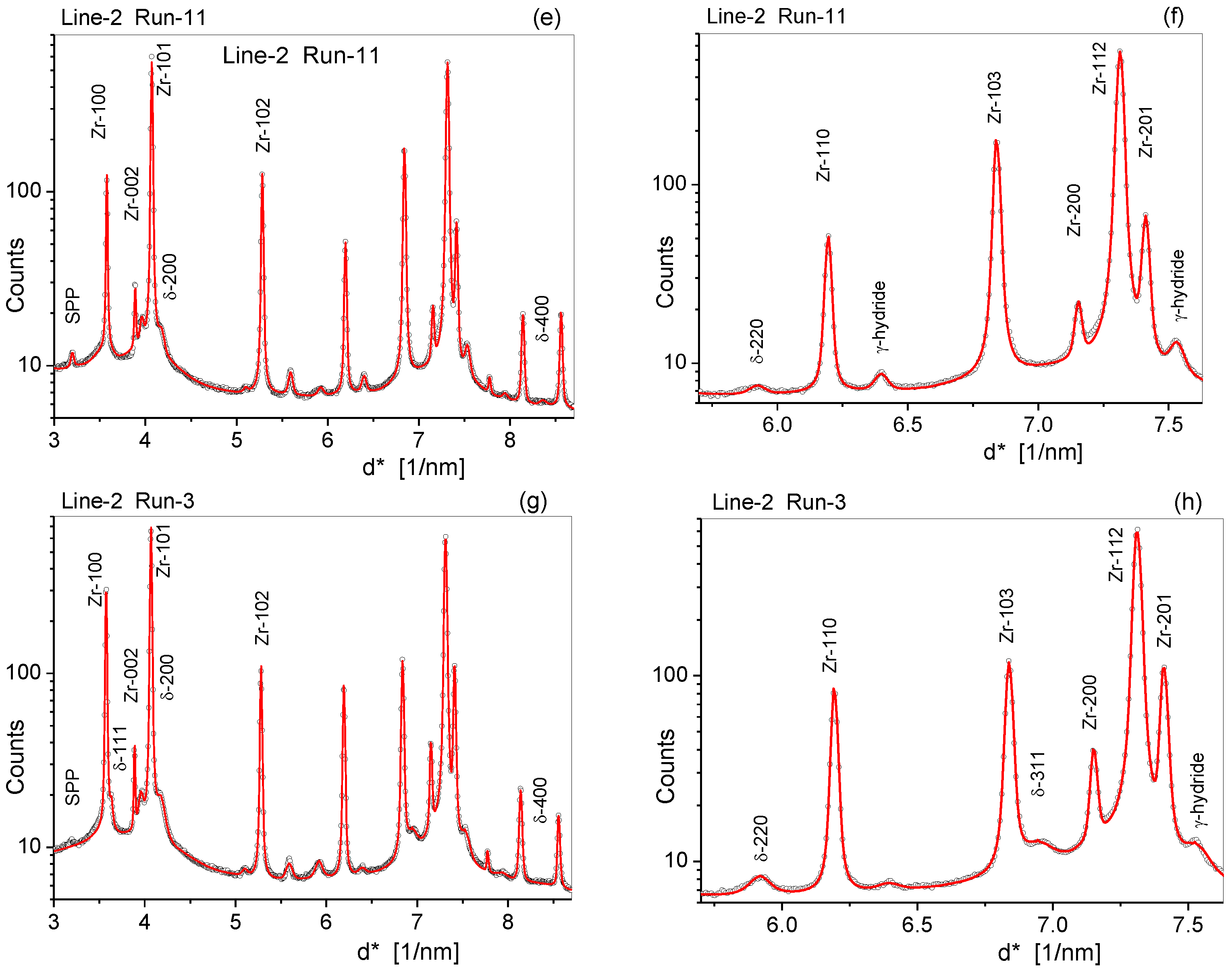
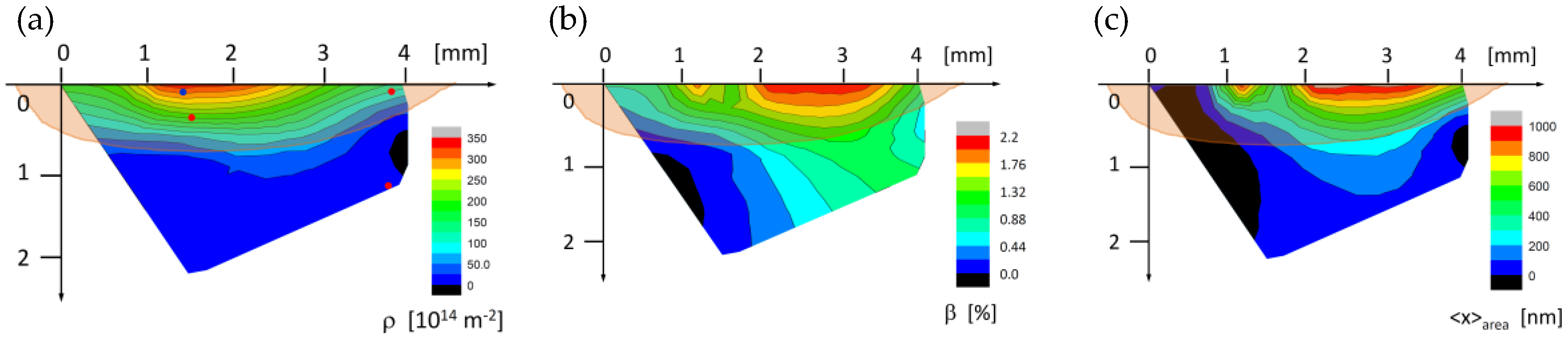
3.1. Experiment
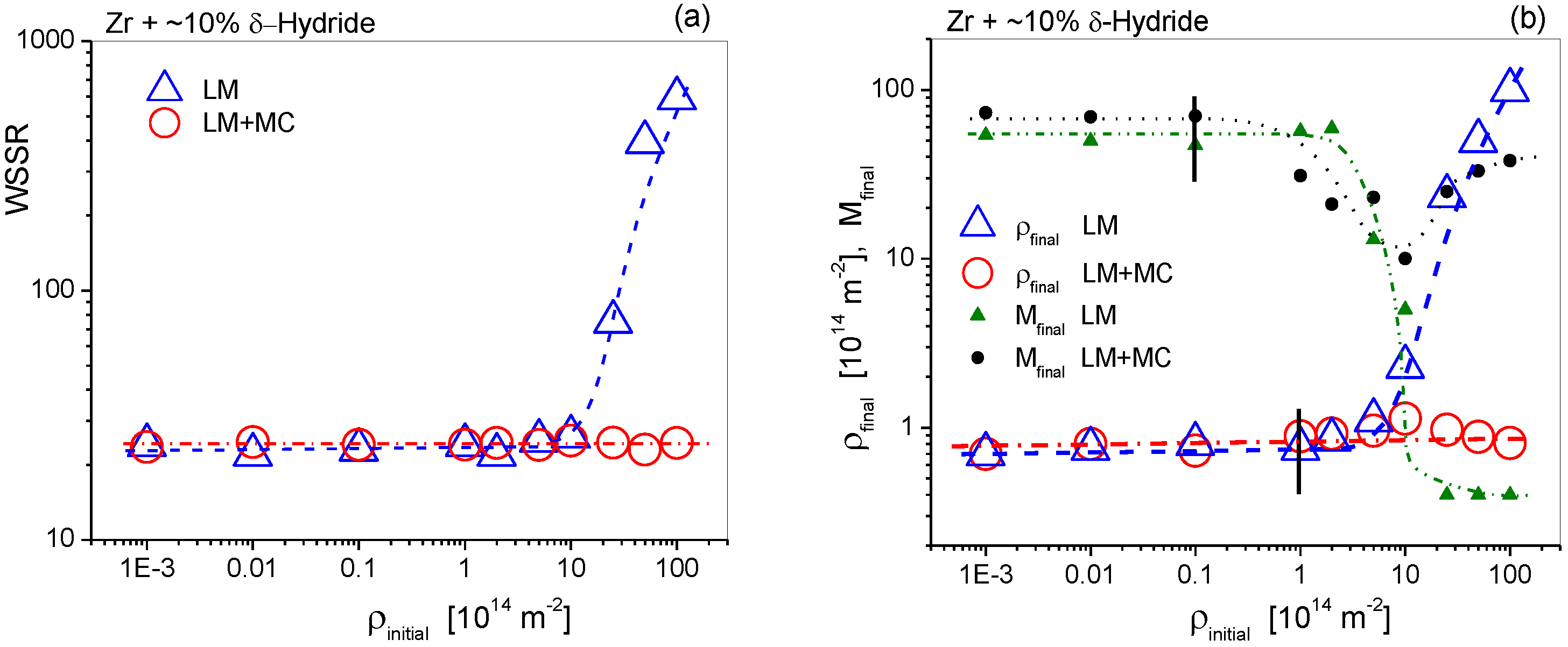
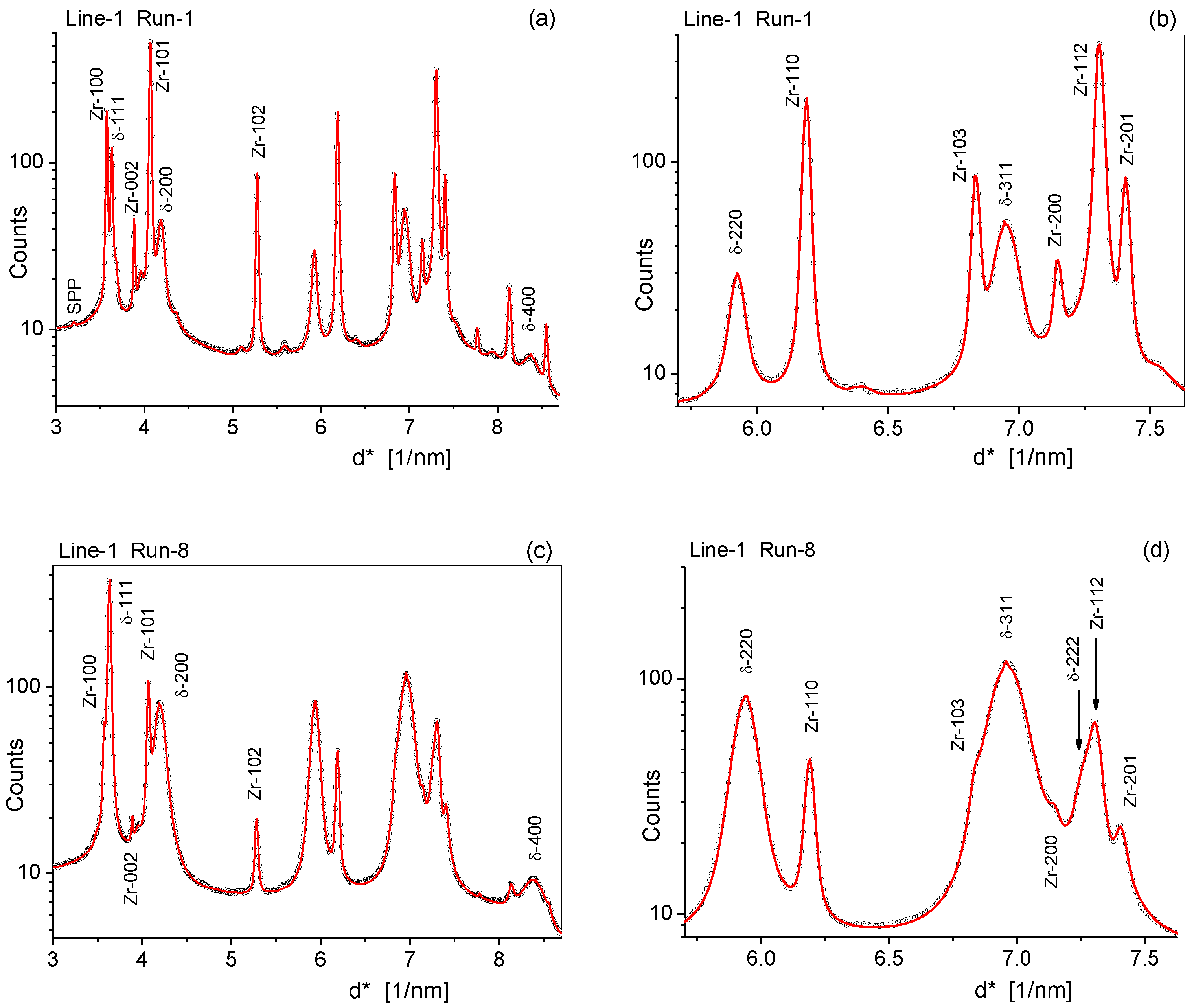
3.2. Results
4. Conclusions
Author Contributions
Funding
Acknowledgments
Conflicts of Interest
References
- Warren, B.E. X-ray studies of deformed metals. Prog. Metal. Phys. 1959, 8, 147–202. [Google Scholar] [CrossRef]
- Wilkens, M. Theoretical aspects of kinematical X-ray diffraction profiles from crystals containing dislocation distributions. In NBS Fundamental Aspects of Dislocation Theory; Simmons, J.A., deWit, R., Bullough, R., Eds.; Spec. Publ. 317, II.: Washington, DC, USA, 1970; pp. 1195–1221. [Google Scholar]
- Wilkens, M. The Determination of Density and Distribution of Dislocations in Deformed Single Crystals from Broadened X-Ray Diffraction Profiles. Phys. Stat. Sol. 1970, 2, 359–370. [Google Scholar] [CrossRef]
- Groma, I. X-ray line broadening due to an inhomogeneous dislocation distribution. Phys. Rev. B 1998, 57, 7535–7542. [Google Scholar] [CrossRef]
- Ungár, T.; Dragomir, I.; Révész, Á.; Borbély, A. The contrast factors of dislocations in cubic crystals: The dislocation model of strain anisotropy in practice. J. Appl. Cryst. 1999, 32, 992–1002. [Google Scholar] [CrossRef] [Green Version]
- Scardi, P.; Leoni, M. Whole powder pattern modelling. Acta Cryst. 2002, 58, 190–200. [Google Scholar] [CrossRef] [PubMed]
- Mittemeijer, E.J.; Scardi, P. (Eds.) Diffraction Analysis of the Microstructure of Materials; Springer: Berlin, Heidelberg, 2004. [Google Scholar]
- Rietveld, H.M. Line profiles of neutron powder-diffraction peaks for structure refinement. Acta Cryst. 1967, 22, 151–152. [Google Scholar] [CrossRef]
- Langford, J.I. A rapid method for analysing the breadths of diffraction and spectral lines using the Voigt function. J. Appl. Cryst. 1978, 11, 10–14. [Google Scholar] [CrossRef]
- Langford, J.I.; Delhez, R.; de Keijser, T.H.; Mittemeijer, E.J. Profile analysis for microcrystalline properties by the Fourier and other methods. Profile analysis for microcrystalline properties by the Fourier and other methods. Aust. J. Phys. 1988, 41, 173–187. [Google Scholar] [CrossRef] [Green Version]
- Balzar, D. Profile fitting of X-ray diffraction lines and Fourier analysis of broadening. J. Appl. Cryst. 1992, 25, 559–570. [Google Scholar] [CrossRef]
- Ribárik, G. Modeling of Diffraction Patterns based on Microstructural Properties. Ph.D. Dissertation, Eötvös University Budapest, Budapest, Hungary, 2008. [Google Scholar]
- Ribárik, G.; Ungár, T. Characterization of the microstructure in random and textured polycrystals and single crystals by diffraction line profile analysis. Mater. Sci. Eng. 2010, 528, 112–121. [Google Scholar] [CrossRef]
- Ungár, T.; Balogh, L.; Ribárik, G. Defect-Related Physical-Profile-Based X-Ray and Neutron Line Profile Analysis. Met. Mater. Transact. 2010, 41, 1202–1209. [Google Scholar]
- Ribárik, G.; Jóni, B.; Ungár, T. Global optimum of microstructure parameters in the CMWP line-profile analysis method by combining Marquardt-Levenberg and Monte-Carlo procedures. J. Mater. Sci. Technol. 2018, 35, 1508–1514. [Google Scholar] [CrossRef] [Green Version]
- James, R.W. The Optical Principles of the Diffraction of X-ray; Bell, G. and Sons Ltd., CERN Document Server: London, UK, 1965. [Google Scholar]
- Bertaut, E.F. Raies de Debye–Scherrer et repartition des dimensions des domaines de Bragg dans les poudres polycristallines. Acta Crystallogr. 1950, 3, 14–18. [Google Scholar] [CrossRef]
- Langford, J.I.; Louër, D.; Scardi, P. Effect of a crystallite size distribution on X-ray diffraction line profiles and whole-powder-pattern fitting. J. Appl. Crystallogr. 2000, 33, 964–974. [Google Scholar] [CrossRef] [Green Version]
- Ungár, T.; Gubicza, J.; Ribárik, G.; Borbély, A. Crystallite size distribution and dislocation structure determined by diffraction profile analysis: Principles and practical application to cubic and hexagonal crystals. J. Appl. Cryst. 2001, 34, 298–310. [Google Scholar] [CrossRef] [Green Version]
- Krivoglaz, M.A.; Ryaboshapka, K.P. Theory of X-ray Scattering by Crystals Containing Dislocations, Randomly Distributed Dislocation Loops. Phys. Met. Metall. 1963, 16, 1–13. [Google Scholar]
- Krivoglaz, M.A. Theory of X-ray and Thermal Neutron Scattering by Real Crystals; Plenum Press: New York, NY, USA, 1996. [Google Scholar]
- Groma, I.; Ungár, T.; Wilkens, M. Asymmetric X-ray Line Broadening of Plastically Deformed Crystals. I. Theory. J. Appl. Cryst. 1988, 21, 47–53. [Google Scholar] [CrossRef]
- Ungár, T.; Groma, I.; Wilkens, M. Asymmetric X-ray Line Broadening of Plastically Deformed Crystals. II. Evaluation Procedure and Application to [001]-Cu Crystals. J. Appl. Cryst. 1989, 22, 26–34. [Google Scholar]
- Borbély, A.; Groma, I. Variance method for the evaluation of particle size and dislocation density from x-ray Bragg peaks. Appl. Phys. Lett. 2001, 79, 1772–1774. [Google Scholar]
- Ungár, T.; Ribárik, G.; Topping, M.; Jones, R.M.A.; Xu, X.D.; Hulse, R.; Harte, H.; Tichy, G.; Race, C.P.; Frankel, P.; et al. Characterizing Dislocation Loops in Irradiated Zr alloys by X-ray Line Profile Analysis of Diffraction Patterns with Satellites. submitted to J. Appl. Cryst 2020. [Google Scholar]
- Groma, I.; Monnet, G.J. Analysis of asymmetric broadening of X-ray diffraction peak profiles caused by randomly distributed polarized dislocation dipoles and dislocation walls. J. Appl. Cryst. 2002, 35, 589–593. [Google Scholar] [CrossRef]
- Velterop, L.; Delhez, R.; de Keijser, T.H.; Mittemeijer, E.J.; Reefman, D. X-ray diffraction analysis of stacking and twin faults in f.c.c. metals: A revision and allowance for texture and non-uniform fault probabilities. J. Appl. Cryst. 2000, 33, 296–306. [Google Scholar] [CrossRef]
- Estevez-Rams, E.; Penton-Madrigal, A.; Lora-Serrano, R.; Martinez-Garcia, J. Direct determination of microstructural parameters from the X-ray diffraction profile of a crystal with stacking faults. J. Appl. Cryst. 2001, 34, 730–736. [Google Scholar] [CrossRef] [Green Version]
- Estevez-Rams, E.; Leoni, M.; Scardi, P.; Aragon-Fernandez, B.; Fuess, H. On the powder diffraction pattern of crystals with stacking faults. Philos. Mag. 2003, 83, 4045–4057. [Google Scholar] [CrossRef]
- Balogh, L.; Ribárik, G.; Ungár, T. Stacking faults and twin boundaries in fcc crystals determined by x-ray diffraction profile analysis. J. Appl. Phys. 2006, 100, 023512. [Google Scholar] [CrossRef]
- Balogh, L.; Tichy, G.; Ungár, T. Twinning on pyramidal planes in hexagonal close packed crystals determined along with other defects by X-ray line profile analysis. J. Appl. Cryst. 2009, 42, 580–591. [Google Scholar] [CrossRef]
- Treacy, M.M.J.; Newsam, J.M.; Deem, M.W. A general recursion method for calculating diffracted intensities from crystals containing planar faults. Proc. Roy. Soc. London 1991, 433, 499–520. [Google Scholar]
- Leineweber, A. Anisotropic diffraction-line broadening due to microstrain distribution: Parametrization opportunities. J. Appl. Cryst. 2006, 39, 509–518. [Google Scholar] [CrossRef] [Green Version]
- Leineweber, A. Anisotropic microstrain broadening in cementite, Fe3C, caused by thermal microstress: Comparison between prediction and results from diffraction-line profile analysis. J. Appl. Cryst. 2012, 45, 944–949. [Google Scholar] [CrossRef]
- Zilahi, G.; Ungár, T.; Tichy, G. A common theory of line broadening and rocking curves. J. Appl. Cryst. 2015, 48, 418–430. [Google Scholar] [CrossRef]
- Hinds, W.C. Aerosol Technology: Properties, Behavior and Measurement of Airborne Particles; Wiley: New York, NY, USA, 1982. [Google Scholar]
- Nabarro, F.R.N. Mathematical theory of stationary dislocations. Adv. Phys. 1952, 1, 269–394. [Google Scholar] [CrossRef]
- Kocks, U.F.; Scattergood, R.O. Elastic Interactions Between Dislocations in a Finite Body. Acta Metall. 1969, 17, 1161–1168. [Google Scholar] [CrossRef]
- Wilkens, M. Das Mittlere Spannungquadrat <σ2> Begrentzt Regellos Verteilter Vesetzungen in einem Zylinderförmigen Körper. Acta Metall. 1969, 17, 1155–1159. [Google Scholar] [CrossRef]
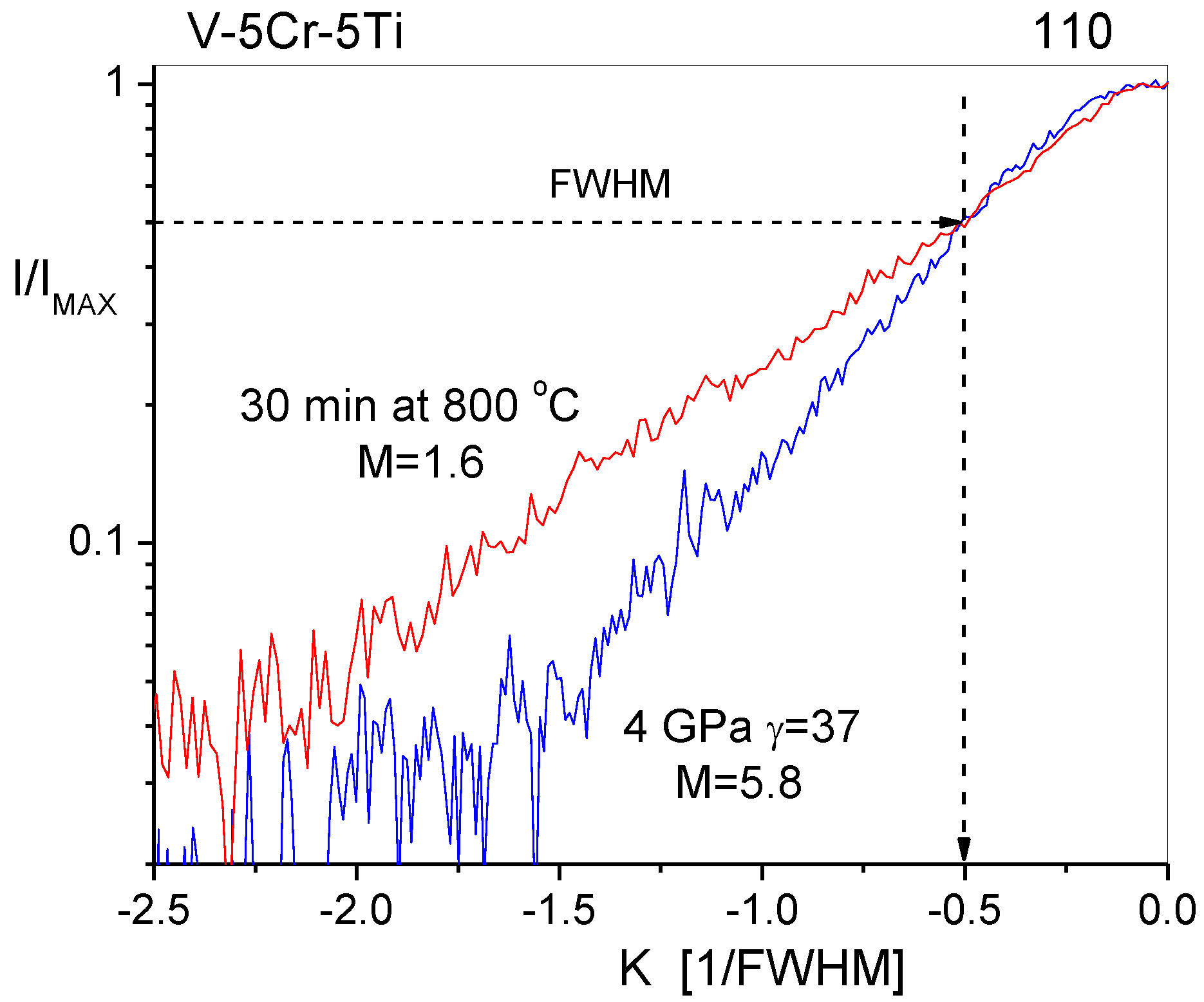
- Fan, Z.; Jóni, B.; Ribárik, G.; Ódor, É.; Fogarassy, Z.; Ungár, T. The microstructure and strength of a V-5Cr-5Ti alloy processed by high pressure torsion. Mater. Sci. Eng. 2019, 758, 139–146. [Google Scholar] [CrossRef] [Green Version]
- Borbély, A.; Dragomir-Cernatescu, I.; Ribárik, G.; Ungár, T. Computer program ANIZC for the calculation of diffraction contrast factors of dislocations in elastically anisotropic cubic, hexagonal and trigonal crystals. J. Appl. Cryst. 2003, 36, 160–162. [Google Scholar] [CrossRef]
- Martinez-Garcia, J.; Leoni, M.; Scardi, P. A general approach for determining the diffraction contrast factorof straight line dislocations. Acta Cryst. 2009, 56A, 109–119. [Google Scholar] [CrossRef]
- Ungár, T.; Tichy, G. The effect of dislocation contrast on X-ray line profiles in untextured polycrystals. Phys. Stat. Sol. 1999, 171, 425–434. [Google Scholar] [CrossRef]
- Dragomir, I.; Ungár, T. Contrast factors of dislocations in the hexagonal crystal system. J. Appl. Cryst. 2002, 35, 556–564. [Google Scholar] [CrossRef]
- Ungár, T.; Castelnau, O.; Ribárik, G.; Drakopoulos, M.; Béchade, J.L.; Chauveau, T.; Snigirev, A.; Snigireva, I.; Schroer, C.; Bacroix, B. Grain to grain slip activity in plastically deformed Zr determined by X-ray micro-diffraction line profile analysis. Acta Mater. 2007, 55, 1117–1127. [Google Scholar] [CrossRef]
- Mujica, N.; Cerda, M.T.; Espinoza, R.; Lisoni, J.; Lund, F. Ultrasound as a probe of dislocation density in aluminum. Cond. Mat. Mtrl. Sci. 2012, 60, 5828–5837. [Google Scholar] [CrossRef] [Green Version]
- Dai, X.; Jiang, F.-L.; Liu, J.; Wu, L.-Y.; Fu, D.-F.; Teng, J.; Zhang, H. Insights into the strain anisotropy models for refined diffraction line profile analysis in cubic metals. Transact. Nonferr. Met. Soc. China 2020. (in the press). [Google Scholar]
- Strutz, T. Data Fitting and Uncertainty (A Practical Introduction to Weighted Least Squares and Beyond), 2nd ed.; Springer Vieweg: New York, NY, USA, 2016. [Google Scholar]
- Kolda, T.G.; Lewis, R.M.; Torczon, V. Optimization by Direct Search: New Perspectives on Some Classical and Modern Methods. SIAM Rev. Soc. Industr. Appl. Mathcs. 2003, 45, 385–482. [Google Scholar] [CrossRef]
- Robert, C.; Casella, G. Monte Carlo Statistical Methods; Springer: Berlin/Heidelberg, Germany, 2004; ISBN 978-1-4757-4145-2. [Google Scholar]
- Levenberg, K. A Method for the Solution of Certain Non-Linear Problems in Least Squares. Quart. Appl. Mathcs. 1944, 2, 164–168. [Google Scholar] [CrossRef] [Green Version]
- Marquardt, D. An Algorithm for Least-Squares Estimation of Nonlinear Parameters. SIAM Rev. Soc. Industr. Appl. Mathcs. 1963, 2, 431–441. [Google Scholar] [CrossRef]
- Tyralis, H.; Koutsoyiannis, D.; Kozanis, S. An algorithm to construct Monte Carlo confidence intervals for an arbitrary function of probability distribution parameters. Comput. Stat. 2013, 28, 1501–1527. [Google Scholar] [CrossRef]
- Müller, P.P.; Schönfeld, B.; Kostorz, G.; Bührer, W. Guinier-Preston I Zones in Al-1.75 at.% Cu Single Crystals. Acta Met. 1989, 37, 2125–2132. [Google Scholar] [CrossRef]
- Ungár, T.; Dubey, P.A.; Kostorz, G. Distortion scattering due to guinier-preston zones in Al-3 at%Ag. Acta Metall. Mater. 1990, 38, 2583–2586. [Google Scholar] [CrossRef]
- Larson, B.C. X-ray diffuse scattering near Bragg reflections for the study of clustered defects in crystalline materials. In Diffuse Scattering and the Fundamental Properties of Materials; Barabash, R.I., Ice, G.E., Turchi, P.E.A., Eds.; Momentum Press: New York, NY, USA, 2009; pp. 139–160. [Google Scholar]
- Seymour, T.; Frankel, P.; Balogh, L.; Ungár, T.; Thompson, S.P.; Jädernäs, D.; Romero, J.; Hallstadius, L.; Daymond, M.R.; Ribárik, G.; et al. Evolution of dislocation structure in neutron irradiated Zircaloy-2 studied by synchrotron x-ray diffraction peak profile analysis. Acta Mater. 2007, 126, 102–113. [Google Scholar] [CrossRef]
- Schönfeld, B.; Kostorz, G. Elastic diffuse scattering of alloys: Status and perspectives. In Diffuse Scattering and the Fundamental Properties of Materials; Barabash, R.I., Ice, G.E., Turchi, P.E.A., Eds.; Momentum Press: New York, NY, USA, 2009; pp. 119–137. [Google Scholar]
- Carpenter, G.J.C.; Zee, R.H.; Rogerson, A. Irradiation Growth of Zirconium Single Crystals. J. Nucl. Mater. 1988, 159, 86–100. [Google Scholar] [CrossRef]
- Onimus, F.; Bechade, J.L. Radiation Effects in Zirconium Alloys. Compr. Nucl. Mater. 2012, 4, 246–273. [Google Scholar]
- Larson, B.C.; Young, F.W., Jr. X-ray diffuse scattering study of irradiation induced dislocation loops in copper. Phys. Stat. Sol. 1987, 104, 273–286. [Google Scholar] [CrossRef]
- Mason, D.R.; Yi, X.; Kirk, M.A.; Dudarev, S.L. Direct observation of size scaling and elastic interaction between nano-scale defects in collision cascades. J. Phys. Cond. Matter. 2014, 110, 375701. [Google Scholar] [CrossRef] [PubMed]
- Dederichs, P.H. Diffuse scattering from defect clusters near Bragg reflections. Phys. Rev. B 1971, 4, 1041–1050. [Google Scholar] [CrossRef]
- Ehrhart, P.; Averback, R.S. Diffuse X-ray scattering studies of neutron- and electron-irradiated Ni, Cu and dilute alloys. Phil. Mag. 1989, 60, 283–306. [Google Scholar] [CrossRef]
- Valizadeh, S.; Ledergerber, G.; Abolhassan, S.; Jädernäs, D.; Dahlbäck, M.; Mader, E.V.; Zhou, G.; Wright, J.; Hallstadius, L. Effects of Secondary Phase Particle Dissolution on the In-Reactor Performance of BWR Cladding. J. ASTM Internat. 2011, 8, 103025. [Google Scholar] [CrossRef]
- Wagner, G.J.; Liu, W.K. Coupling of atomistic and continuum simulations using a bridging scale decomposition. J. Comput. Phys. 2003, 190, 249–274. [Google Scholar] [CrossRef]
- Seif, D.; Po, G.; Mrovec, M.; Lazar, M.; Elsässer, C.; Gumbsch, P. Atomistically enabled nonsingular anisotropic elastic representation of near-core dislocation stress fields in α-iron. Phy. Rev. B 2015, 91, 184102. [Google Scholar] [CrossRef] [Green Version]
- Topping, M.; Harte, A.; Ungár, T.; Race, C.P.; Dumbill, S.; Frankel, P.; Preuss, M. The effect of irradiation temperature on damage structures in proton-irradiated zirconium alloys. J. Nucl. Mater. 2019, 514, 358–367. [Google Scholar] [CrossRef] [Green Version]
- Jones, R.M.A. The Effect of Niobium on the Microstructural Evolution of Zirconium Alloys during Proton Irradiation. Ph.D. Dissertatio, The University of Manchester, Manchester, UK, 2019. [Google Scholar]
- Vicente-Alvarez, M.A.; Santisteban, J.R.; Domizzi, G.; Almer, J. Phase and texture analysis of a hydride blister in a Zr–2.5%Nb tube by synchrotron X-ray diffraction. Acta Mater. 2011, 59, 2210–2220. [Google Scholar] [CrossRef]
- Vicente-Alvarez, M.A.; Santisteban, J.R.; Vizcaíno, P.; Ribárik, G.; Ungár, T. Quantification of dislocations densities in zirconium hydride by X-ray line profile analysis. Acta Mater. 2016, 117, 1–12. [Google Scholar] [CrossRef] [Green Version]
- Domizzi, G.; Enrique, R.A.; Ovejero-Garcia, J.; Buscaglia, G.C. Blister growth in zirconium alloys: Experimentation and modeling. J. Nucl. Mater. 1996, 229, 36–47. [Google Scholar] [CrossRef]
- Qin, W.; Szpunar, J.A.; Kozinsk, J. Hydride-induced degradation of zirconium alloys: A criterion for complete ductile-to-brittle transition and its dependence on microstructure. Proc. Roy. Soc. 2015, 471, 20150192. [Google Scholar] [CrossRef]


© 2020 by the authors. Licensee MDPI, Basel, Switzerland. This article is an open access article distributed under the terms and conditions of the Creative Commons Attribution (CC BY) license (http://creativecommons.org/licenses/by/4.0/).
Share and Cite
Ribárik, G.; Jóni, B.; Ungár, T. The Convolutional Multiple Whole Profile (CMWP) Fitting Method, a Global Optimization Procedure for Microstructure Determination. Crystals 2020, 10, 623. https://doi.org/10.3390/cryst10070623
Ribárik G, Jóni B, Ungár T. The Convolutional Multiple Whole Profile (CMWP) Fitting Method, a Global Optimization Procedure for Microstructure Determination. Crystals. 2020; 10(7):623. https://doi.org/10.3390/cryst10070623
Chicago/Turabian StyleRibárik, Gábor, Bertalan Jóni, and Tamás Ungár. 2020. "The Convolutional Multiple Whole Profile (CMWP) Fitting Method, a Global Optimization Procedure for Microstructure Determination" Crystals 10, no. 7: 623. https://doi.org/10.3390/cryst10070623