Multiple Twisted Chiral Nematic Structures in Cylindrical Confinement

Abstract

In this article, we theoretically and numerically study the chirality and saddle-splay elastic constant ($K_{24})$-enabled stability of multiple twist-like nematic liquid crystal (LC) structures in cylindrical confinement. We focus on the so-called radially z-twisted (RZT) and radially twisted (RT) configurations, which simultaneously exhibit twists in different spatial directions. We express the free energies of the structures in terms of dimensionless wave vectors, which characterise the structures and play the roles of order parameters. The impact of different confinement anchoring conditions is explored. A simple Landau-type analysis provides an insight into how different model parameters influence the stability of structures. We determine conditions for which the structures are stable in chiral and also nonchiral LCs. In particular, we find that the RZT structure could exhibit macroscopic chirality inversion upon varying the relevant parameters. This phenomenon could be exploited for the measurement of$K_{24}$.

1. Introduction

Chirality is pervasive in nature and refers to cases where an object and its mirror image are different [1,2,3]. It signals the absence of inversion symmetry, giving rise to a right-handed and left-handed appearance and behaviour. Chirality is present throughout physics and often impacts or even dominates numerous important natural phenomena. For example, chiral symmetry plays an important role in the Standard Model of physics [4]. The functionalities of several essential components of biological cells rely heavily on chirality [3]. Furthermore, it could be exploited in various technological and medical applications [5,6,7]. By exploiting chirality, one could engineer new materials with extraordinary properties (e.g., metamaterials exhibiting negative refractive index [8]). Therefore, a deep understanding of chirality and its related emergent behaviours is of interest throughout the physical and biological sciences.

However, several issues related to chirality remain unresolved, even at a fundamental level. For instance, the molecular origins of chirality and the relative role of chiral symmetry-breaking remain an open problem [9]. In particular, the mechanisms involved in the transfer of chirality from microscopic to macroscopic level [10] are not sufficiently understood. Convenient systems with which to gain a deeper understanding of the latter features are chiral uniaxial nematic liquid crystals (NLCs; a list of abbreviations appears at the end), one of the simplest representatives of anisotropic soft materials [11,12]. These systems are relatively easily accessible experimentally, structural changes can be triggered by relatively weak external stimuli, and a macroscopic chiral response can be achieved using different pathways.

Uniaxial NLCs consist of approximately rod-shaped objects that, in bulk equilibrium, exhibit long-range orientational order and the absence of translational order [11]. The local orientational order is commonly described by the mesoscopic nematic director field $\overrightarrow{n}$, exhibiting head-to-tail invariance–the states $\pm \overrightarrow{n}$ are physically equivalent. In the classical Oseen–Frank approach [11], the elastic free energy is expressed as the sum of the so-called splay, twist, bend, and saddle-splay contributions, weighted by Frank splay ($K_{11}$), twist ($K_{22}$), bend ($K_{33}$), and saddle-splay ($K_{24}$) elastic constants. These contributions penalise different elastic distortions and determine equilibrium nematic director field patterns.

In the bulk achiral nematic phase, $\overrightarrow{n}$ is spatially homogeneously aligned along a single symmetry-breaking direction. In a simple chiral nematic (also referred to as the cholesteric) phase, in the bulk equilibrium structure, $\overrightarrow{n}$ twists in space, describing a helix where $\overrightarrow{n}$ is always perpendicular to the helix axis. This structure exhibits only a single twist (i.e., it twists only along one spatial direction) deformation.

Even more complex structures could be formed in chiral materials exhibiting a propensity for saddle-splay deformations [13,14], which in liquid crystals (LCs) is controlled by the saddle-splay elastic constant $K_{24}.$ The energy elastic term weighted by $K_{24}$ equals the Gaussian curvature of a hypothetical local surface [11], whose surface norma is determined by $\overrightarrow{n}.$ This term is different from zero for the nematic structures displaying, e.g., double twist-like deformations, in which $\overrightarrow{n}$ varies in two orthogonal directions. Consequently, such structures could decrease the overall free energy for a large enough value of $K_{24}$. Note that the saddle-splay elastic term can be expressed as pure divergence, and can be mathematically integrated out to the surface confining the LC. Therefore, it affects LC order through boundary conditions. In most cases, the saddle-splay-enforced boundary tendency is masked by stronger surface anchoring conditions. For this reason, the $K_{24}$ contribution is often ignored in theoretical modelling [11,14]. Its magnitude range is determined by Ericksen’s inequality [15] $0<K_{24}<K_{1,2}^{\left(min\right)},$ where $K_{1,2}^{\left(min\right)}$ corresponds to the lower elastic modulus of the twist ($K_{22}$) and splay ($K_{11}$) elastic deformations. Furthermore, due to the anchoring strength-“masking” effect it is relatively difficult to measure the magnitude of $K_{24}.$ In other words, for strong enough anchoring [11] (i.e., RW/K>>1, where R is the characteristic confinement length, K stands for the average Frank elastic constant, and W is the surface anchoring strength coefficient), the surface anchoring contribution overrides the competing $K_{24}$ contribution in the relevant surface Euler-Lagrange equilibrium equations. Consequently, only a few experimental measurements of $K_{24}$ have been reported [16,17,18]. Several of these measurements report values of $K_{24}$ that are close to $K_{1,2}^{\left(min\right)}.$

We note that a natural decomposition of representative nematic elastic distortions was recently proposed by Selinger [19]. Four bulk elastic normal modes were introduced, representing distinct irreducible representations of the rotational symmetry group characterising NLC symmetry. These are referred to as the double splay, double twist, bend, and biaxial splay mode, which could be separately and independently excited. On the contrary, the classical (single) splay, (single) twist, bend, and saddle-splay distortions [11,19] are, in general, coupled. For instance, the saddle-splay term can be expressed as a sum of double splay, double twist, and biaxial splay mode.

Nematic structures exhibiting nonplanar 3D nematic distortions (e.g., double twist deformations) impose elastic frustrations, which can be resolved in bulk by introducing assemblies of topological defects [20,21], as manifested in Blue Phases (BPs) [22,23,24]. In NLCs, a description of defects would require a more complex structural description in terms of the tensor nematic order parameter [11], which allows for the local melting of the LC order and the presence of biaxial states [25]. On the other hand, such deformations could be realised without defects in appropriate confinement geometries, where cylindrical confinements [26,27,28,29,30,31] are most often used. Note that stable 3D realisations of topological defects are of interest for science in general. For instance, if physical fields represent fundamental entities of nature [32], then topological defects might represent [33] fundamental particles in the conventional “particle”-based natural description.

In this contribution, we consider nematic structures within chiral LCs in cylindrical confinement. We focus on the (meta) stability of multiple twist-type structures, which exhibit variations in the nematic molecular field simultaneously in at least two orthogonal spatial directions. We show that several structural properties can arise in the context of a simple Landau-type model. A more general analysis is carried out numerically. We determine regimes where one could observe a change in the handedness of structures by varying relevant material parameters. Furthermore, we determine regimes in which the saddle-splay elasticity sensitively controls the stability of competing structures.

2. Results

Of interest are defect-free spontaneously twisted NLC structures within an infinitely long cylinder of radius R. For this reason, we use cylindrical coordinates {$r,\phi ,z$}, defined by the unit vector triad {${\overrightarrow{e}}_r,{\overrightarrow{e}}_{\phi },{\overrightarrow{e}}_z$}. We consider two different ansatzes, which give a good approximation of two qualitatively different families of solutions that are expected to be stable for the geometries and boundary conditions of interest well [26,27].

The first class is represented by [26,27]

$${\overrightarrow{n}}^{\left(i\right)}=cos\psi sin\mathsf{\Omega }{\overrightarrow{e}}_r+sin\psi sin\mathsf{\Omega } {\overrightarrow{e}}_{\phi }+cos\mathsf{\Omega } {\overrightarrow{e}}_z,$$

(1)

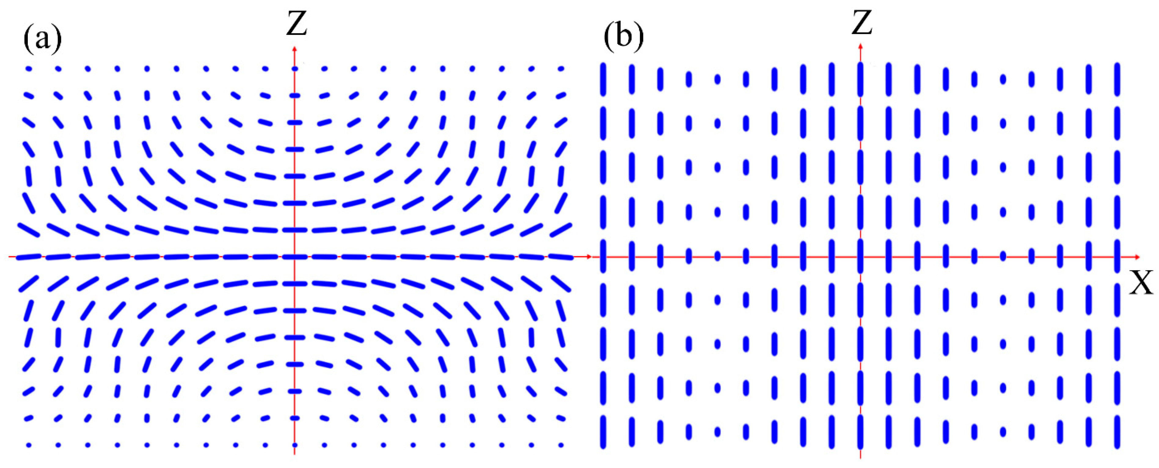
where $\psi =q_{1}z-\phi$, $\mathsf{\Omega }=\frac{\pi }{2}-q_{2}r sin\psi ,$ the wave vectors $q_1$ and $q_2$ are variational parameters. A typical representative structure is shown in Figure 1a and in the Supplementary Materials.

In the Cartesian coordinates {x, y, z} the ansatz reads ${\overrightarrow{n}}^{\left(i\right)}=\cos \left(q_{1}z\right) sin\mathsf{\Omega }{\overrightarrow{e}}_x+sin\left(q_{1}z\right) sin\mathsf{\Omega } {\overrightarrow{e}}_y+cos\mathsf{\Omega } {\overrightarrow{e}}_z$ Cases $q_1\ne 0$ and $q_2\ne 0$ determine multiple twisted solutions. In these patterns, which we refer to as radially z-twisted (RZT) structures, twist deformation is realised both along the ${\overrightarrow{e}}_r$ and ${\overrightarrow{e}}_z$ directions [26]. This ansatz also encompasses single twisted structures. For example, for $q_2=0$ a structure twisting around the z axis is expressed as

$${\overrightarrow{n}}^{\left(i\right)}=cos(q_{1}z-\phi ) {\overrightarrow{e}}_r+\sin \left(q_{1}z-\phi \right) {\overrightarrow{e}}_{\phi },$$

(2)

which corresponds to a classical cholesteric solution with wave vector $q_1$.

The second family of solution corresponds to the radially twisted (RT) structures [26,27], where the twist is realised along ${\overrightarrow{e}}_r$, see Figure 1b. For this purpose, we use the ansatz

$${\overrightarrow{n}}^{\left(ii\right)}=sin\alpha {\overrightarrow{e}}_{\phi }+cos\alpha {\overrightarrow{e}}_z.$$

(3a)

Here, $\alpha =\alpha \left(r\right)$ and to avoid a singularity at the cylinder axis we impose the condition α(0) = 0. Previous numerical studies [26,31] have revealed that the dependence of α(r) is roughly linear in r, even for large twists of $\stackrel{\rightharpoonup }{n}$. Consequently, we use the approximation:

$$\alpha =q_{RT}r.$$

(3b)

These structures were numerically studied in Refs. [26,27,31], where their stability was analysed. Our proposed ansatzes mimic the numerically obtained structures for the anchoring conditions of interest well for relatively small wave vectors and in the approximation of equal Frank elastic constants $K_{11}=K_{22}=K_{33}$. In the cases examined, the free energies of structures obtained (i) numerically by solving the relevant Euler–Lagrange equations or (ii) using our ansatzes differ by less than 10%. By using the analytical ansatzes, we were able to carry out a Landau-type approach, which enabled a more detailed insight into the stability of structures of interest for various different material-dependent parameters.

In the following, we use the approximation of equal elastic constants $K\equiv K_{11}=K_{22}=K_{33}$, but allow $K_{24}\ne K$. At the cylinder’s lateral wall, $r=R$, we impose, for the positive anchoring strength, W > 0 (see Equation (19) in Methods) either (a) homeotropic anchoring $\left(\overrightarrow{e}={\overrightarrow{e}}_r\right)$, (b) tangential anchoring along ${\overrightarrow{e}}_z$ (i.e., $\left(\overrightarrow{e}={\overrightarrow{e}}_z\right)$, or (c) tangential anchoring along ${\overrightarrow{e}}_{\phi }\left(\overrightarrow{e}={\overrightarrow{e}}_{\phi }\right)$. We henceforth refer to these cases as (a) homeotropic, (b) zenithal tangential), and (c) azimuthal tangential anchoring, respectively. For $W<0$, these cases correspond to isotropic tangential anchoring in a plane with a normal surface in the direction $\overrightarrow{e}.$ Note that, in our study, the latter case is sensible only for condition (a).

For convenience, we introduce the following dimensionless quantities: Q = qR, Q₁ = q₁R, Q₂ = q₂R, Q_RT = q_RTR, k₂₄ = K₂₄/K, w = RW/K, and the dimensionless free energy is scaled in units of $F_0=\pi KH.$ Therefore $F\to F/F_0$, where H is the height of the cylinder. For numerical convenience, we suppose that H is either large in comparison with the period $p=2\pi /q_1$, or an integer number of p.

2.1. Free Energies of Structures

Using the ansatzes Equations (1) and (3) and the scaling described above, we calculate the free energies F of the structures (see Equation (1)). For later convenience, the energies are decomposed as $F^{\left(i\right)}=F_e^{\left(i\right)}+F_s^{\left(i\right)}$ and $F^{\left(ii\right)}=F_e^{\left(ii\right)}+F_s^{\left(ii\right)}$ for the first (RZT) and second class (RT) of solutions, respectively.

We consider first the family of solutions labelled by ${\overrightarrow{n}}^{\left(i\right)}$ (Equation (1)). The elastic contribution is

$$F_e^{\left(i\right)}=\frac{{\left(Q-Q_2\right)}^2}{2}+\frac{Q_1^2{Q}_2^2}{8}+\frac{Q_1}{2}\left(\frac{Q_1}{2}+\left(1-k_{24}\right)Q_2-Q\right)\left(1+\frac{J_1\left(2Q_2\right)}{Q_2}\right)$$

(4)

Now let $F_s^{\left(i\right)}$stand for the interface contribution, which is different for (a) homeotropic ($F_s^{\left(i\right)}=F_{s,h}^{\left(i\right)}$), (b) zenithal ($F_s^{\left(i\right)}=F_{s,z}^{\left(i\right)}$), and (c) azimuthal $F_s^{\left(i\right)}=F_{s,\phi }^{\left(i\right)}$ anchoring:

$$F_{s,h}^{\left(i\right)}=\frac{3w}{4}-\frac{w}{4}\frac{J_1\left(2Q_2\right)}{Q_2}$$

(5a)

$$F_{s,z}^{\left(i\right)}=\frac{w}{2}-\frac{w}{2}{J}_0\left(2Q_2\right),$$

(5b)

$$F_{s,\phi }^{\left(i\right)}=\frac{3w}{4}+w\left(\frac{J_1\left(2Q_2\right)}{4Q_2}-\frac{J_0\left(2Q_2\right)}{2}\right).$$

(5c)

where J₀ and J₁ stand for the Bessel functions in the order of zero and one, respectively.

The second class of solutions is determined by the elastic term:

$$F_e^{\left(ii\right)}=\frac{1}{2}{\left(Q+Q_{RT}\right)}^2+\left(1-k_{24}+\frac{Q}{Q_{RT}}\right)si{n}^2{Q}_{RT}+{{\displaystyle \int }}_0^1\frac{si{n}^2\left(Q_{RT}x\right)}{x}dx,$$

(6)

and surface contributions:

$$F_{s,h}^{\left(ii\right)}=w,$$

(7a)

$$F_{s,z}^{\left(ii\right)}=w si{n}^2{Q}_{RT},$$

(7b)

$$F_{s,\phi }^{\left(ii\right)}=w co{s}^2{Q}_{RT}$$

(7c)

We obtain solutions by varying the variational parameters $Q_1, Q_2$and $Q_{RT}$ for the given material properties (determined by Q, $k_{24}, w$) and boundary conditions.

Of interest is the determination of regimes where radially z-twisted (RZT) or radially twisted (RT) structures are stable. We first perform an analytic analysis of these structures, where we expand the free energies in the limit of relatively small dimensionless wave numbers $Q_1, Q_2$and $Q_{RT}$. Then, we perform a more detailed stability analysis numerically.

2.2. Landau-Type Analysis

We first consider RZT (class 1) structures using the ansatz of Equation (4). By minimising the total free energy $F^{\left(i\right)}$ with respect to $Q_1$, it follows that:

$$Q_1=\frac{Q+\left(k_{24}-1\right)Q_2}{1+\frac{Q_2^2}{2\left(1+\frac{J_1\left(2Q_2\right)}{Q_2}\right)}}$$

(8)

In the following, we examine only the regimes of relatively low wave vectors $Q_2$ (i.e., $Q_2\ll 1$), for which Equation (8) yields:

$$Q_1~Q+\left(k_{24}-1\right)Q_2-\frac{Q_2^{2}Q}{4}.$$

(9)

Taking this into account, we expand $F^{\left(i\right)}$ up to the fourth power in $Q_2.$ It follows that:

$$\begin{gathered} F_h^{\left(i\right)}=\frac{w}{2}+\frac{{\left(Q-Q_2\right)}^2}{2}-k_{24}Q{Q}_2+\frac{8k_{24}-4k_{24}^2+2Q^2+w}{8}{Q}_2^2+\frac{Q\left(k_{24}-1\right)}{2}{Q}_2^3+ \\ \frac{24-48k_{24}+24k_{24}^2-5Q^2-2w}{96}{Q}_2^4, \end{gathered}$$

(10a)

$$\begin{gathered} F_z^{\left(i\right)}=\frac{{\left(Q-Q_2\right)}^2}{2}-k_{24}Q{Q}_2+\frac{4k_{24}-2k_{24}^2+Q^2+2w}{4}{Q}_2^2+\frac{Q\left(k_{24}-1\right)}{2}{Q}_2^3+ \\ \frac{24-48k_{24}+24k_{24}^2-5Q^2-12w}{96}{Q}_2^4, \end{gathered}$$

(10b)

$$F_{\phi }^{\left(i\right)}=\frac{w}{2}+\frac{{\left(Q-Q_2\right)}^2}{2}-k_{24}Q{Q}_2+\frac{8k_{24}-4k_{24}^2+3w}{8}{Q}_2^2+\frac{Q\left(k_{24}-1\right)}{2}{Q}_2^3+\frac{24-48k_{24}+24k_{24}^2-10w}{96}{Q}_2^4.$$

(10c)

where $F_h^{\left(i\right)}$, $F_z^{\left(i\right)}$, and $F_{\phi }^{\left(i\right)}$ denote $F^{\left(i\right)}$for homeotropic, zenithal, and azimuthal anchoring, respectively. We thus obtain a Landau-type expansion of the form $F^{\left(i\right)}=F_0^{\left(i\right)}+{\alpha }_1{Q}_2+{\alpha }_2{Q}_2^2+{\alpha }_3{Q}_2^3+{\alpha }_4{Q}_2^4$, where $Q_2$ and {${\alpha }_1,{\alpha }_2,{\alpha }_3,{\alpha }_4$} play the role of order parameter and Landau expansion coefficients, respectively.

For achiral LCs ($Q=0$), one obtains:

$$F_h^{\left(i\right)}=\frac{w}{2}+\frac{8k_{24}-4k_{24}^2+w+4}{8}{Q}_2^2+\frac{24-48k_{24}+24k_{24}^2-2w}{96}{Q}_2^4,$$

(11a)

$$F_z^{\left(i\right)}=\frac{4k_{24}-2k_{24}^2+2w+4}{4}{Q}_2^2+\frac{24-48k_{24}+24k_{24}^2-12w}{96}{Q}_2^4,$$

(11b)

$$F_{\phi }^{\left(i\right)}=\frac{w}{2}+\frac{8k_{24}-4k_{24}^2+3w+4}{8}{Q}_2^2+\frac{24-48k_{24}+24k_{24}^2-10w}{96}{Q}_2^4.$$

(11c)

The spatially homogeneous order becomes unstable with respect to the RZT class of solutions where the coefficients ${\alpha }_2$ that weight the $Q_2^2$ contribution in Equation (11) change signs. From the condition ${\alpha }_2=0$, one could deduce a critical value, $k_{24}$, above which the RZT structures become stable:

$$k_{24}^{\left(h\right)}=1+\sqrt{1+\frac{w}{4}}$$

(12a)

$$k_{24}^{\left(z\right)}=1+\sqrt{1+w}$$

(12b)

$$k_{24}^{\left(\phi \right)}=1+\sqrt{1+\frac{3w}{4}}$$

(12c)

where $k_{24}^{\left(h\right)}, k_{24}^{\left(z\right)},$ and $k_{24}^{\left(\phi \right)}$ determine the critical values of $k_{24}$ for homeotropic, zenithal, and azimuthal anchoring, respectively. Note that, in the approximation of equal elastic constants, the Ericksen critical value of $K_{24}$ is given by $k_{24}^{\left(e\right)}=2$. Therefore, in the absence of chirality, $K_{24}$ could trigger twisted structures only for $w<0$, which, in our modelling, is physically meaningful for the case given by Equation (12a).

Next, we focus on the RT structures using the ansatz of Equation (3). When $Q_{RT}\ll 1$, it follows that:

$$F_e^{\left(ii\right)}~\frac{Q^2}{2}+2Q{Q}_{RT}+\left(2-k_{24}\right)Q_{RT}^2-\frac{Q{Q}_{RT}^3}{3}+\frac{\left(k_{24}-\frac{5}{4}\right)}{3}{Q}_{RT}^4.$$

(13)

It is easy to estimate the equilibrium value of the chirality wave number Q_RT of the RT structure if both Q and Q_RT are small. We use Equations (13) and (7) and free energy minimisation yields:

$$Q_{RT}=-Q/\left(2+\Delta -k_{24}\right),$$

(14)

with $\Delta =0$ for homeotropic anchoring, and $\Delta =\pm w$ for tangential anchorings (positive sign for zenithal anchoring and negative sign for azimuthal anchoring). Note that Equation (14) is valid only in the limit when $\left|Q_{RT}\right|<1$.

For achiral LCs it follows that:

$$F_h^{\left(ii\right)}~w+\left(2-k_{24}\right)Q_{RT}^2+\frac{\left(k_{24}-\frac{5}{4}\right)}{3}{Q}_{RT}^4.$$

(15a)

$$F_z^{\left(ii\right)}~\left(2-k_{24}+w\right)Q_{RT}^2+\frac{\left(k_{24}-\frac{5}{4}-w\right)}{3}{Q}_{RT}^4.$$

(15b)

$$F_{\phi }^{\left(ii\right)}~w+\left(2-k_{24}-W\right)Q_{RT}^2+\frac{\left(k_{24}-\frac{5}{4}+w\right)}{3}{Q}_{RT}^4.$$

(15c)

The critical conditions read:

$$k_{24}^{\left(h\right)}=2,$$

(16a)

$$k_{24}^{\left(z\right)}=2+w,$$

(16b)

$$k_{24}^{\left(\phi \right)}=2-w.$$

(16c)

Therefore, in achiral LCs, the saddle-splay elasticity may trigger an RT structure below $k_{24}^{\left(e\right)}=2$ only in the case of azimuthal anchoring.

2.3. Numerical Analysis

We next explore the (meta) stability of double-twist structures in chiral LCs. Of particular interest is the determination of regimes in which the reversal of macroscopic chirality could be realised by varying a relevant parameter. Note that our estimates work well for dimensionless wave vectors less than one. Most of the “interesting” phenomena are realised in this regime. Therefore, results obtained for wave vectors larger than one are only indicative.

2.3.1. RZT Structure: Homeotropic Anchoring

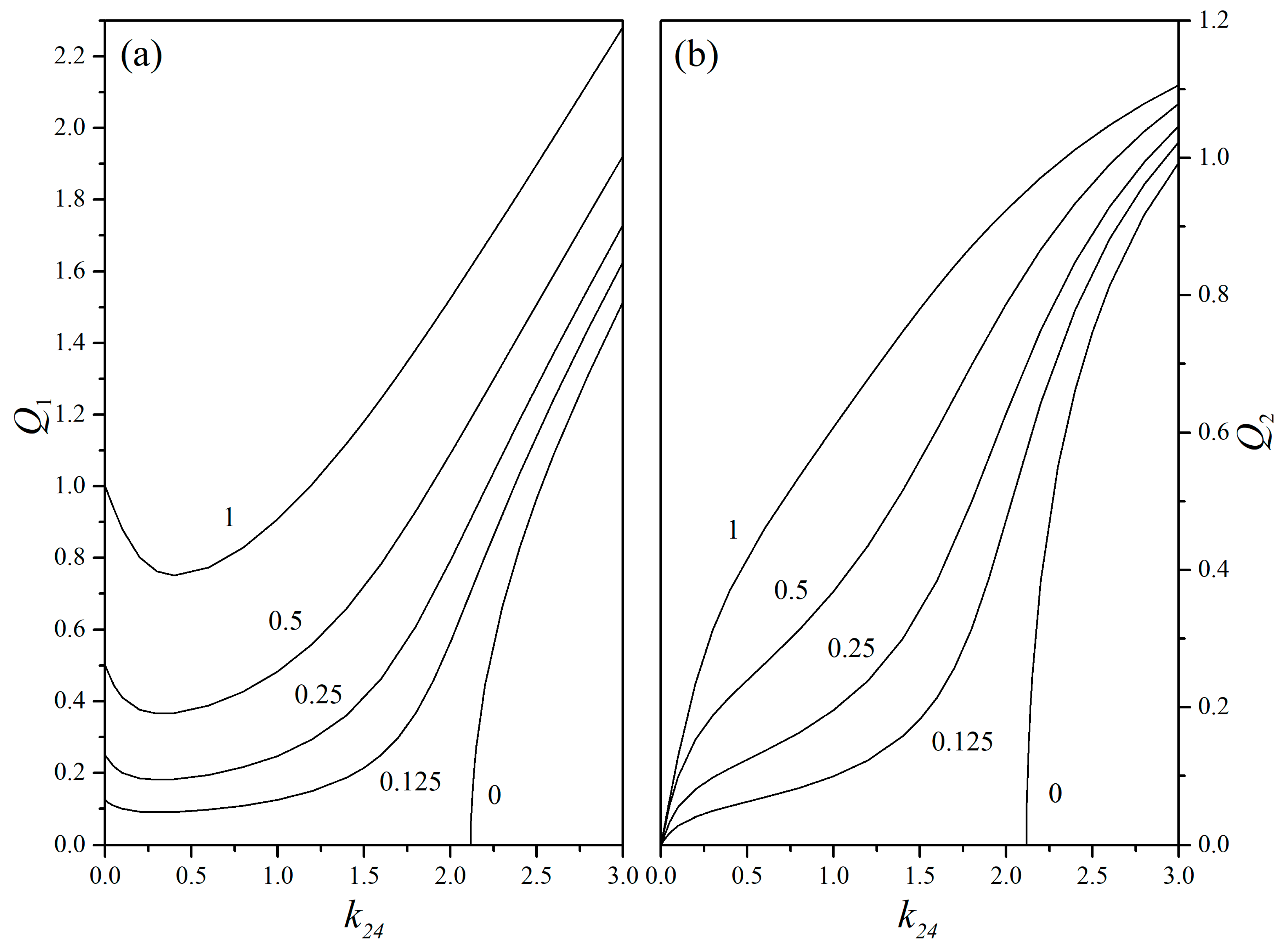
We focus first on RZT (class 1) structures and homeotropic anchoring. Of interest is the exploration of the impact of the saddle-splay constant k₂₄ and intrinsic chirality Q for relatively weak anchoring, which we set to w = 1. In Figure 2, we plot Q₁ and Q₂ equilibrium values (i.e., they determine local minima in F) varying Q between zero and one. For the case Q = 0 (achiral nematic) the RZT structures could be triggered only in the regime $k_{24}>k_{24}^{\left(e\right)}\equiv 2$. However, for chiral LCs, $k_{24}$ efficiently promotes the stability of RZT structures well below $k_{24}^{\left(e\right)}$. Furthermore, for $k_{24}$= 0, it holds that Q₂ = 0 and Q₁ = Q. This solution corresponds to the classic cholesteric structure; see Equation (2). Graphs in Figure 2 also reveal that the value of k₂₄ can be extracted experimentally.

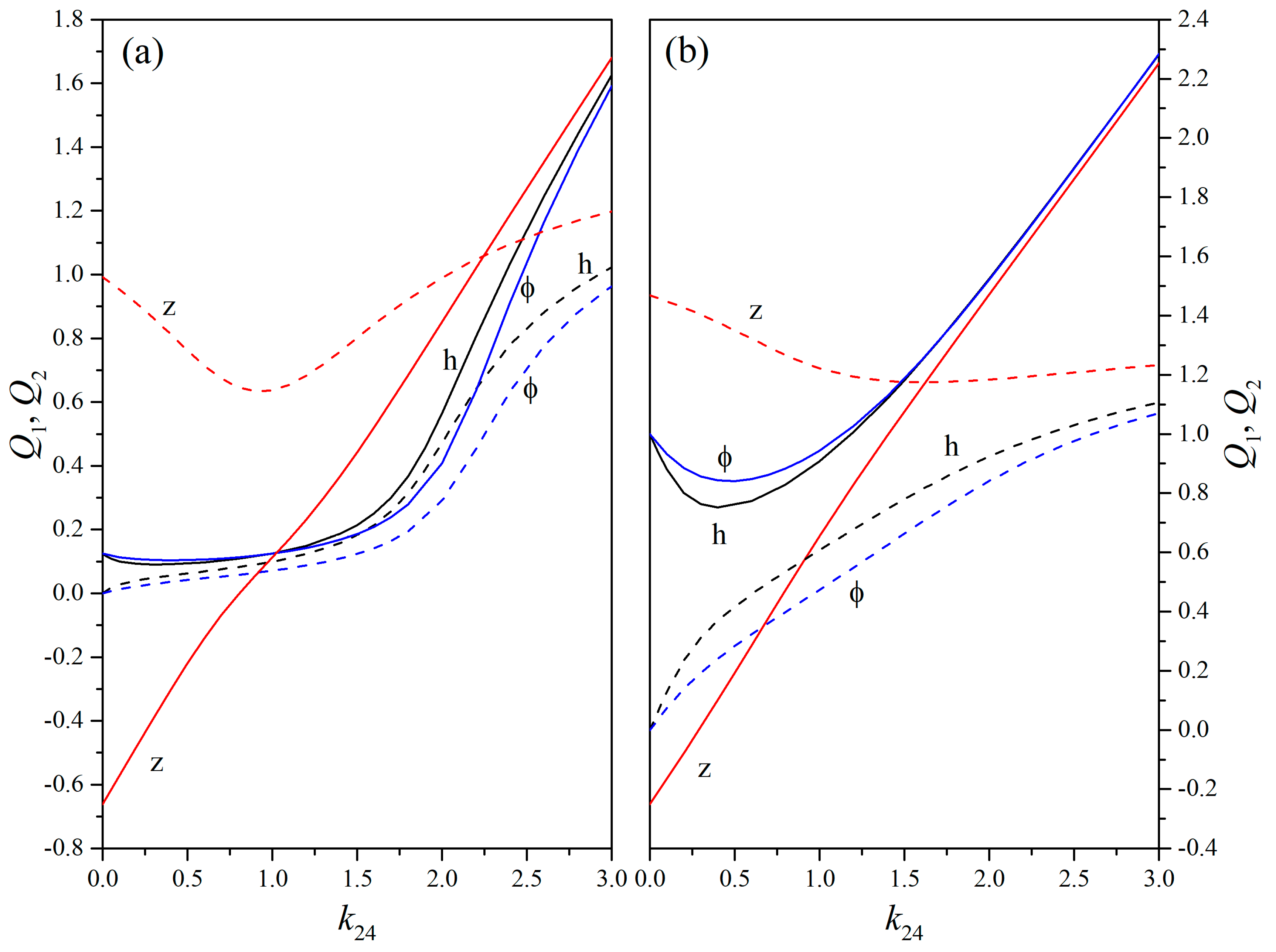
2.3.2. RZT Structure: Tangential Anchoring

For tangential anchorings, the configurational variability of RZT structures is much more complex. This is illustrated in Figure 3, where we plot the dependencies of Q₁(k₂₄) and Q₂(k₂₄) on all studied anchoring conditions for two significantly different values of Q, viz., Q = 0.125 and Q = 1. The behaviour is roughly similar for homeotropic and azimuthal anchoring, whereas, for zenithal anchoring, qualitatively different features emerge. In particular, Q₁ could even change signs at a critical value of k_24, which we denote by $k_{24}^{\left(c\right)}$. Similarly, for a given value of k₂₄, this crossover could be achieved by varying Q, and we label the corresponding critical value as $Q_c.$

Note that the value of $k_{24}^{\left(c\right)}$ depends relatively strongly on Q. Because the uniaxial twist with Q₁ = 0 can be observed easily by polarised optical microscopy, this phenomenon may be exploited to measure the splay−bend elastic constant. This is illustrated in Figure 4, where we plot the Q_c(k₂₄) dependence for different anchoring strengths. Experimentally, one could vary Q by adding a chiral dopant to LC. The reversal of the sign of Q₁ exists in the interval 0 < $k_{24}$ < 1, well below $k_{24}^{\left(e\right)}$. In the strong anchoring limit W → ∞, the graph Q_c(k₂₄) approaches a straight line.

2.3.3. Relative Stability of RZT and RT Structures

The minimum energies (corresponding to local minima in varying variational parameters) of both types of structures (RZT and RT) were compared for different sets of parameters. In general, homeotropic anchoring favours RZT configurations. This is obvious since the nematic director of the RT structure is always parallel to the boundary plane at the cylinder boundary. On the other hand, for both types of tangential anchoring, the stability regimes of different structures depend on a specific set of parameters, k₂₄, Q and w. Due to a broad parameter space, we limit our analysis to a few cases relevant to our study. 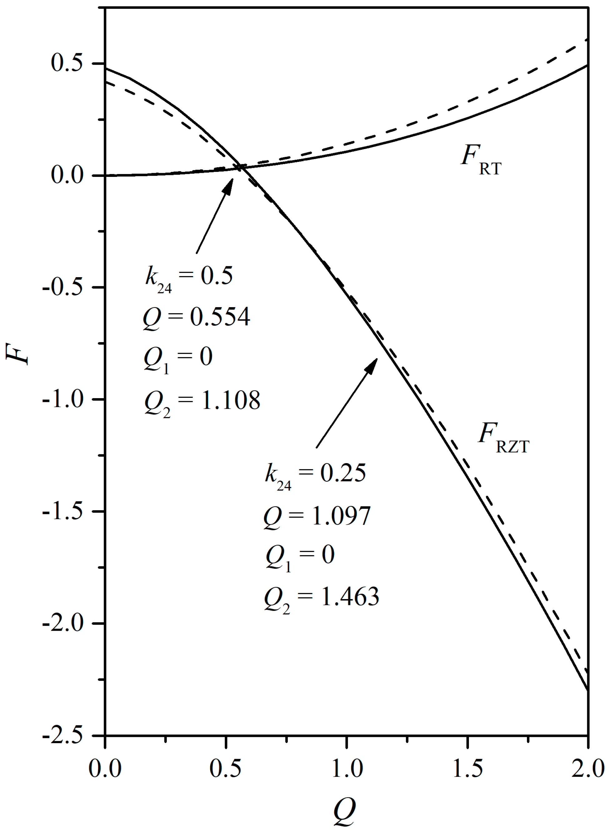For example, Figure 4 reveals the parameters for which Q₁ = 0 (chirality reversal) is realised for the RZT configuration for zenithal anchoring. It is essential to compare its free energy with the competitive RT structure. Some representative examples are depicted in Figure 5 and Figure 6. In Figure 5, we plot the minimum energies of the competing structures on varying Q for k₂₄ = 0.5 and weak (w = 1) zenithal anchoring for the case exhibiting chirality reversal. In this case, the RZT structure with Q₁ < 0 is metastable with respect to RT. However, Figure 5 illustrates the existence of a regime for which the configuration with Q₁ < 0 is stable for k₂₄=0.25. Thus, chirality reversal may be found experimentally in this case. The arrows in Figure 5 approximately indicate the energy of the RZT structure at the reversal of the sign of Q₁, together with the calculated chirality parameters. For lower values of Q, it holds that Q₁ < 0, and vice versa. Although the energies for k₂₄ = 0.25 and 0.5 are not very different, the critical value of Q (Q_c = Q, where Q₁ changes signs) differs significantly: Q_c = 0.554 for k₂₄ = 0.5, whereas Q_c = 1.097 for k₂₄ = 0.25.

Note that we have tested the stability of RZT and RT structures with respect to the nonchiral escaped radial structure [18], in which the director profile exhibits cylindrical symmetry. It tends to be radially oriented at the cylinder wall and gradually reorients along the z axis on approaching the cylinder axis. For homeotropic anchoring, it exists for $w=RW/K>1$, and its free energy is given by [18]:

$$\frac{F}{\pi KH}=3-k_{24}-\frac{1}{\sigma }$$

(17)

where $\sigma =w+k_{24}-1$. In the region of interest, this structure is energetically costlier with respect to the competing RZT or RT structure.

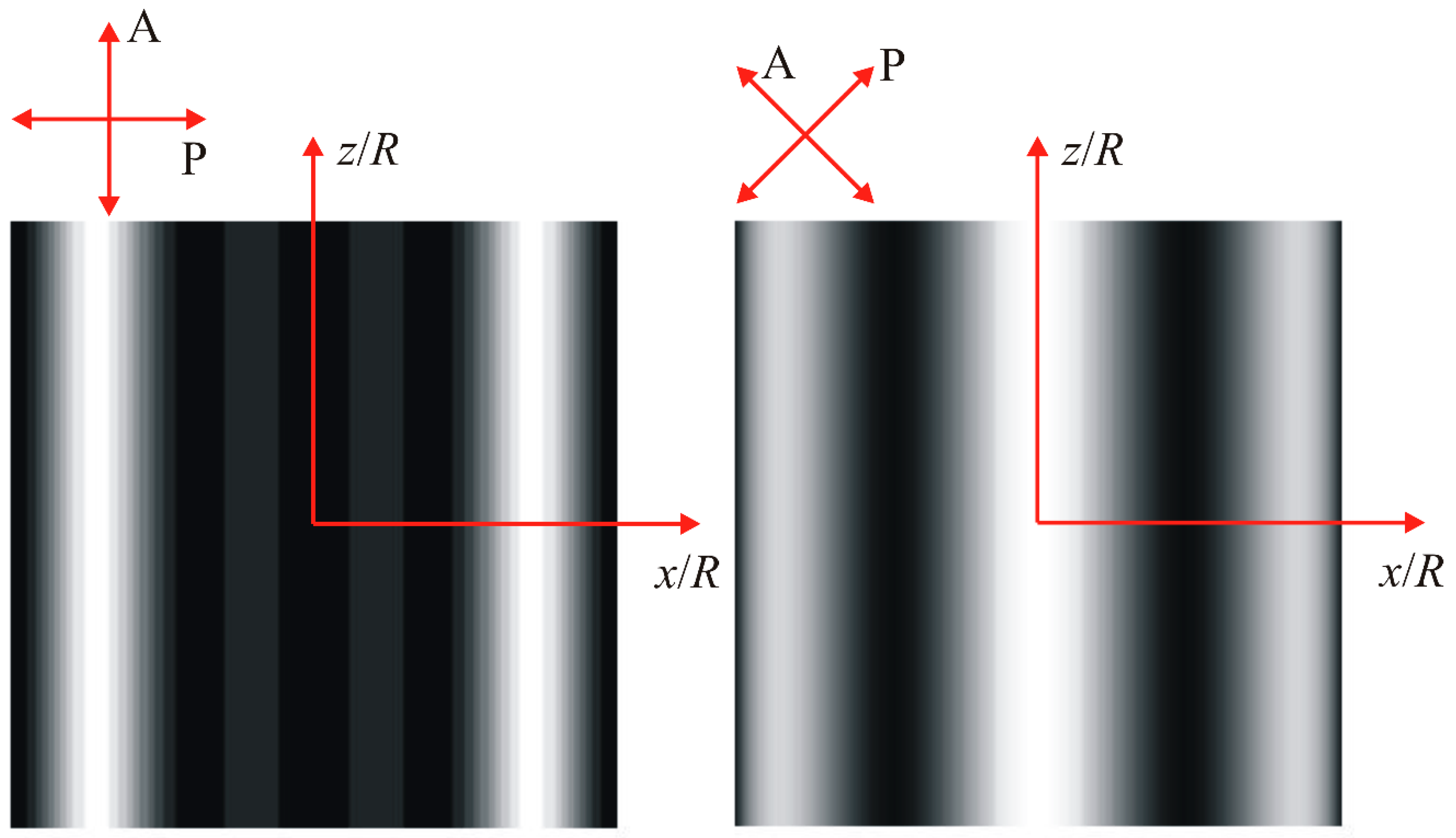
Finally, in Figure 7 and Figure 8, we show calculated optical polarising microscopy patterns for the competing RZT and RT structures for two different polarisation directions of the polariser and analyser, where we set Q₁ = Q₂ = Q_RT = 1. Simulation details are described in [29]. The polarisations of the polariser and analyser are mutually perpendicular. The angle between the polariser and x-axis (horizontal axis) is 0° or 45°. One sees that the textures are significantly different and that one could easily distinguish these structures by using polarising optical microscopy.

3. Conclusions

We studied the impact of chirality, the saddle-splay elastic constant and anchoring conditions on the (meta) stability of radially z-twisted (RZT), and radially twisted (RT) configurations realised in a cylindrical confinement of the radius, R. We used the Oseen–Frank uniaxial description in terms of the nematic director field. Such a description is sensible because we do not consider configurations exhibiting topological defects, which would require the local melting of the nematic order or the presence of biaxiality. Furthermore, we used the approximation of equal Frank elastic constants $K_{11}=K_{22}=K_{33}\equiv K$. We expressed the free energy of structures in terms of dimensionless wavenumbers $Q_1,$ $Q_2, Q_{RT},$ which represent order parameters in our Landau-type analysis. The parameter space controlling the relative stability of the structures consists of the dimensionless chirality $Q=Rq$, dimensionless saddle-splay constant $k_{24}=K_{24}/K$, and dimensionless anchoring strength $w=\frac{RW}{K}.$

We found that, in the absence of chirality, the RZT structure could be (meta) stable (fulfilling the Ericksen inequality $k_{24}<k_e\equiv 2$) only for isotropic tangential anchoring, provided that $k_{24}>1+\sqrt{1-\left|w\right|/4}$. On the other hand, the RT structure could be (meta) stable for the azimuthal anchoring condition and $k_{24}>2-\left|w\right|$. However, chirality enables the stability of RZT structures for $k_{24}$ values in the interval $k_{24}\in \left[0,2\right]$. Furthermore, for $Q_{RT}<1$, we found that the RT structures exhibit the wave vector $Q_{RT}~-Q/\left(2+\Delta -k_{24}\right)$, where (i) $\Delta =0$, (ii) $\Delta =\left|w\right|$, (iii) $\Delta =-\left|w\right|$ for (i) homeotropic, (ii) zenithal, and (iii) azimuthal anchoring, respectively. In addition, we observed that the RZT configuration could exhibit a sign reversal of the wave vector for zenithal anchoring upon varying a relevant control parameter. This approach could be exploited for the experimental determination of $K_{24}$ values, which still require considerably more exploration.

Note that multiple twisted structures could be exploited in several applications because their wave vectors can be adjusted to the optically visible regime. Such 3D structures could stabilise the lattices of disclinations, as manifested in the Blue Phases and related Skyrmion-like structures. The study of the latter structures could also provide an understanding of the fundamental workings of their nature, which is still lacking.

4. Methods

We used the Oseen–Frank continuum approach [11], where nematic structures are expressed in terms of the nematic director field $\overrightarrow{n}$. The free energy of confined NLCs is expressed as:

$$F={\displaystyle \iiint }{f}_e{d}^3\overrightarrow{r}+{\displaystyle \iint }{f}_s{d}^2\overrightarrow{r}.$$

(18)

The first and second integrals are carried over the LC volume and over a NLC-confining surface. The quantities $f_e$ and $f_s$determine the elastic and NLC-confining surface free energy density contributions.

The elastic term reads:

$$f_e=\frac{K_{11}}{2}{\left(\nabla .\overrightarrow{n}\right)}^2+\frac{K_{22}}{2}{\left(\overrightarrow{n}.\nabla \times \overrightarrow{n}+q\right)}^2+\frac{K_{33}}{2}{\left|\overrightarrow{n}\times \nabla \times \overrightarrow{n}\right|}^2-\frac{K_{24}}{2}\nabla .\left(\overrightarrow{n}\nabla .\overrightarrow{n}+\overrightarrow{n}\times \nabla \times \overrightarrow{n}\right).$$

(19)

The elastic response is determined by the splay (K₁₁), twist (K₂₂), bend (K₃₃) and saddle-splay (K₂₄) elastic constant, respectively. The wave vector $q$ reflects the inherent LC chirality.

We modeled the surface interaction term using a simple Rapini–Papoular [11] description:

$$f_s=\frac{W}{2}\left(1-{\left(\overrightarrow{n}.\overrightarrow{e}\right)}^2\right).$$

(20)

Here, the unit vector $\overrightarrow{e}$ is commonly referred to as the easy axis. For instance, for W > 0, the corresponding free energy is locally minimised if $\overrightarrow{n}$ is aligned along $\overrightarrow{e}.$ Furthermore, for W < 0, the term is minimised for $\overrightarrow{n}\perp \overrightarrow{e}.$