What EBSD and TKD Tell Us about the Crystallography of the Martensitic B2-B19′ Transformation in NiTi Shape Memory Alloys

Abstract

The complex and intricate microstructure of B19′ martensite in shape memory nickel titanium alloys is generally explained with the Phenomenological Theory of Martensitic Crystallography (PTMC). Over the last decade, we have developed an alternative approach that supposes the existence of a “natural” parent–daughter orientation relationship (OR). As the previous TEM studies could not capture the global crystallographic characteristics of the B2→B19′ transformation required to discriminate the models, we used Electron BackScatter Diffraction (EBSD) and Transmission Kikuchi Diffraction (TKD) to investigate a polycrystalline NiTi alloy composed of B19′ martensite. The EBSD maps show the large martensite plates and reveal the coexistence of different ORs. The TKD maps permit us to image the “twins” and confirm the continuum of orientations suspected from EBSD. The results are interpreted with the alternative approach. The predominant OR in EBSD is the “natural” OR for which the dense directions and dense planes of B2 and B19′ phases are parallel—i.e., (010)_B19′//(110)_B2 and [101]_B19′//[$\overline{1}$11]_B2. The natural OR was used to automatically reconstruct the prior parent B2 grains in the EBSD and TKD maps. From the distortion matrix associated with this OR, we calculated that the habit plane could be (1$\overline{1}$2)_B2//(10$\overline{1}$)_B19′. The traces of these planes are in good agreement with the EBSD maps. We interpret the other ORs as “closing-gap” ORs derived from the natural OR to allow the compatibility between the distortion variants. Each of them restores a parent symmetry element between the variants that was lost by distortion but preserved by correspondence.

1. Introduction

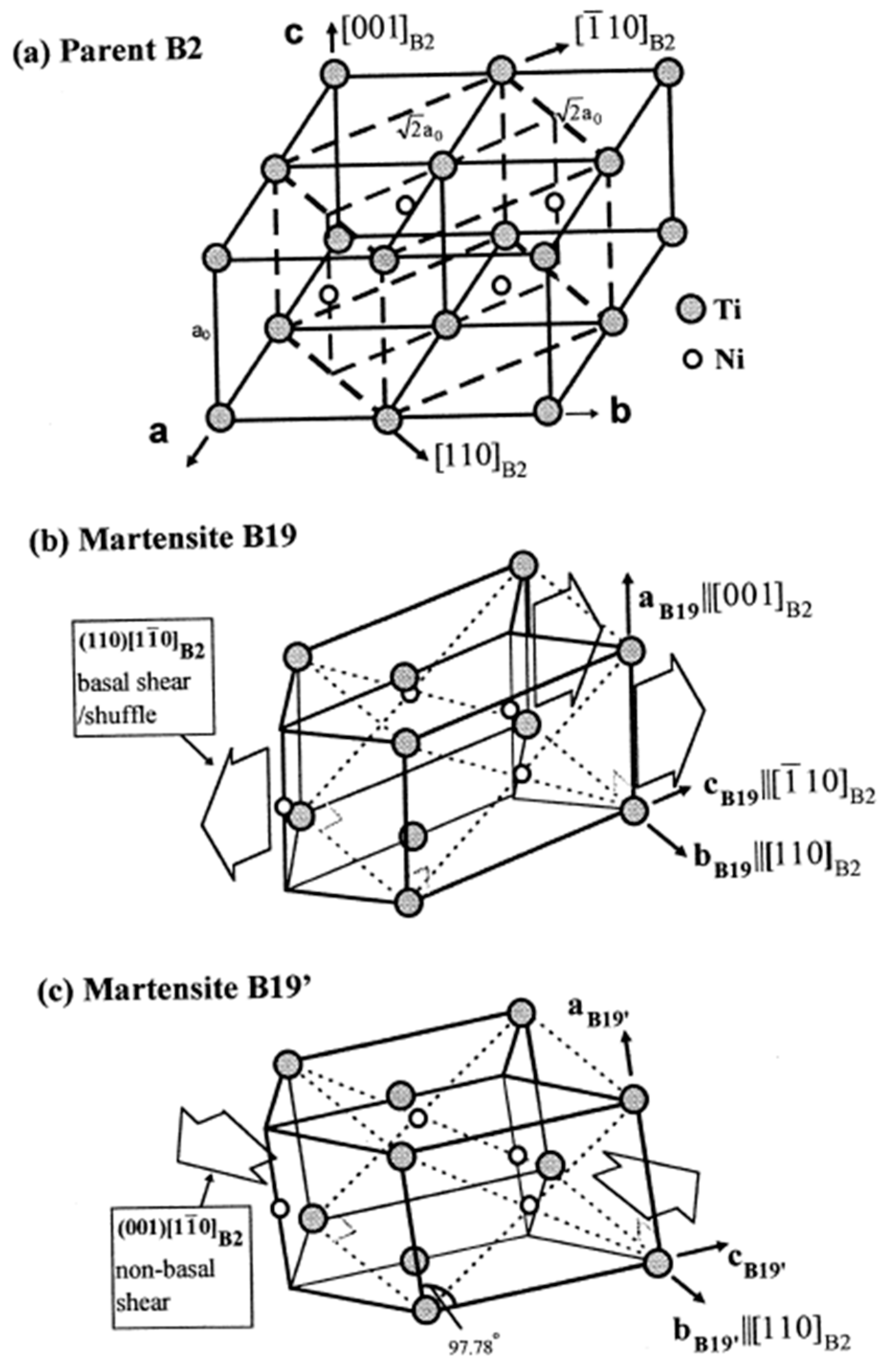
1.1. A Brief Review of the Crystallography of NiTi Alloys

Nickel titanium shape memory alloys and their extraordinary properties were discovered in 1963 [1], which is quite late in the long history of metallurgy. At that time, the research on martensite in steels was well advanced; the Crystallographic Theory of Martensitic Crystallography (PTMC) had already been developed by two different groups in 1953–1954 [2,3]. This theory is based on matrix calculations and elementary crystallography. Since the morphology of martensite is often plate or lenticular, PTMC assumes that the habit plane (the plane of the plate or the mid-rib of the lenticle) is the plane of an “invariant plane strain”; consequently, that martensite results from an invariant plane strain deformation. This deformation mode is a composition of a simple shear along the habit plane (no volume change) and an extension or a contraction perpendicularly to the habit plane (that gives the volume change of the transformation). It can be obtained only by assuming that the martensite deformation is a composite made of two individual lattice distortions. By polar decomposition, these lattice distortions can be expressed in the form of a rotation composed with a Bain stretch. The Bain stretch is a symmetric matrix inferred by finding the “easiest” way to convert the Bravais lattice of the parent phase into that of the daughter phase. The name “Bain” is given in honor to Edgar C. Bain, who first proposed in 1924 how a face-centered-cubic (fcc) crystal could be transformed into a body-centered-cubic (bcc) crystal [4]. In order to maintain the compatibility between the lattice distortions of the two variants, PTMC assumes that there exists a simple shear transformation between them. This shear is called a “lattice invariant strain” or “lattice invariant deformation” because dislocation gliding or deformation twinning are considered as possible candidates. The list of possible twins is calculated with the twinning theory developed since the end of the 19th century by researchers such as Mügge [5], Friedel [6], Kihô [7], and Bevis and Crocker [8] (see also [9,10]). The twins are often ranked according to their shear values and shuffle complexity. They are also classified into two categories: type I and type II. If two crystals are in mirror symmetry through a reticular plane (h,k,l), they form a {h,k,l} type I twin. If they are misoriented by a 180° rotation around a reticular axis [u,v,w], they form a <u,v,w> type II twin. The compatibility plane i/j between the twin-related variants i and j in the composite martensite is simply called a “junction plane”. It is also the twin plane for variants linked by a type I twin. The PTMC mainly consists of solving equations in which the average deformation of a martensite plate made of two twin-related variants i and j in x and (1 − x) volume proportion is an invariant plane strain. The invariant plane of the “composite” martensite (i,j) is the habit plane. Because of the symmetries of the austenite, there are different but symmetry-equivalent habit planes called “habit plane variants”.

Excellent didactic reviews of the early versions of the PTMC can be found in Refs [11,12,13]. The theory is very popular in metallurgy, as exampled by this enthusiastic sentence “the most impressive, but often complex and mathematically inscrutable, theory of phase transformations ever produced-the phenomenological theory of martensite crystallography (the PTMC)” [12]. The microstructure of martensite in NiTi alloys is very thin and intricate; its observation has required transmission electron microscopy (TEM). The experimental result are nearly systematically interpreted with the PTMC. One major researcher on NiTi is Otsuka; he used TEM with Shimizu [14], a former colleague of Prof. Nishiyama, who is well-known for his important contribution to martensite in steels and great supporter of the PTMC [15]. Otsuka et al. [14] could show that (11$\overline{1}$)_B19′ was a twinning plane between some variants. Other studies showed other junction planes, such as the (001)_B19′, (100)_B19′, and (011)_B19′ planes [16,17]. These twins were identified as type I twins. Knowles and Smith [18] were the first to report a <011>_B19′ type II twin in NiTi alloys. The type II twins are quite rare in metals and this discovery attracted the attention of the specialists of NiTi. According to the twinning theory, the shear plane of a type II twin, which is also the junction plane between the two variants, is irrational. For <011>_B19′ type II twins, the expected junction plane is close to (0.72,1,$\overline{1}$)_B2 ≈ (3,4,$\overline{4}$)_B2. This plane was later confirmed by other experimental studies, for example by High Resolution Transmission Electron Microscopy (HRTEM) [19,20]. The interface is decomposed into edges and ledges on lower indices planes. It remains the subject of theoretical studies [21].

One of the missing points at that time for a complete confirmation of the PTMC was the experimental determination of the habit plane(s) of the B19′ martensite. Their measurements were made by analyzing by optical microscopy the martensite traces at the surfaces of single crystals. In 1984, in a study about the effect of grain size and orientation on the shape memory effect, Saburi [22] mentioned an habit plane close to (4,5,11)_B2 without showing any detail. The same year, Miyazaki et al. [23] reported a study completely dedicated to the question. Despite a large scattering of ±4°, they could identify two groups around (5,6,14)_B2 and around (8,9,14)_B2. They compared them to the PTMC predictions by considering the two lattice invariant strains already assessed by Knowles and Smith [18]—i.e., the (11$\overline{1}$)_B19′ type I twins and the <011>_B19′ type II twins. Among the habit planes “predicted” by the PTMC, the one closest to the experience is (0.215,0.405,0.888)_B2. The authors concluded that “The agreement between theory and experiment for solution-treated specimens is fairly good but not so good as for the case of Au-Cd alloy, while that for aged specimens are poor. The causes of the deviation of observed values from the theoretical one are not known.” A few years later, in 1989 Miyazaki, Otsuka, and Wayman [24] reported a study on the self-accommodation of variants and measured experimental habit planes close to (0.39,0.48,0.78)_B2, which is an intermediate of the two previously reported habit planes. They concluded that “the calculated habit planes […] fit well with the experimentally obtained ones”. This shift of statements between the two studies (“fairly good” or “poor” to “well”) is really surprising because it was clear in the pole figures showing both the experimental and predicted habit planes that the difference was actually not small. A simple calculation shows that the angle between the PTMC-predicted (0.215,0.405,0.888)_B2 habit planes and the experimental (0.39,0.48,0.78)_B2 is 12°. It is 6° with (4,5,11) or (5,6,14), and 10° with (8,9,14). Such difference is beyond the experimental error. A larger scattering of the orientations was reported by Matsumoto et al. [25], which allowed the authors to notice a better agreement between some habit planes chosen in the cloud of experience and the PTMC predictions.

Besides the inaccurate prediction of the habit planes, PTMC is not clear about the choice that should be made in the long list of deformation twins or glide systems. Only the twins with the lowest shears are considered in general, but the shear values s are, however, quite high. For example, Knowles and Smith calculated s = 0.31 for (11$\overline{1}$) type I twinning and s = 0.28 for <011>_B19′ type II twins. These values are greater than those of extension twins in magnesium, and are quite close the twinning shear reported in fcc and bcc metals. In these metals, the twins are not reversible because of the accommodation dislocations generated in the surrounding matrix. It is thus not clear why the “twins” are reversible in NiTi shape memory alloys (a phenomenon called “detwinning” or “variant reorientation”), whereas they are not reversible in usual metals. An explanation could be that the type of atomic bonding in ordered NiTi intermetallic alloys are “stronger” than in metals and thus less prone to plasticity, but this point remains untreated by the PTMC, which only considers the lattices. In order to distinguish the B19′ martensite variants from real deformation twins, the B19′ variants are often called “transformation twins”. This name will be justified by the modern mathematical treatments of PTMC detailed in the next section. Whatever the names, some of the observed junction planes, such as (100) _B19′ and (001)_B19′, disagree with PTMC because they do not lead to any solution in the PTMC equations [26]. It is funny to note that some researchers then escape from this issue by calling these variants “deformation twins” [26] as a new terminology in place of the “transformation twins”. All the “twins” reported in the TEM studies, whatever their names, were observed in quenched alloys without any prior or post macroscopic mechanical deformation, and nothing in their morphology permits us to distinguish them.

PTMC evolved at the turn of 1990s [27,28,29,30] with a mathematical formulation of the compatibility criterion, and more recently, with the supercompatibility criterion [31]. In this modern version, the lattice invariant strain is not any more a choice made in the list of deformation twins but becomes an output of the calculations. The main idea is that the distortion matrices ${\mathbf{F}}_i$ and ${\mathbf{F}}_j$ of two variants, i and j, respectively, are expressed by polar decomposition in the forms ${\mathbf{Q}}_i{\mathbf{U}}_i$ and ${\mathbf{Q}}_j{\mathbf{U}}_j$, respectively, with ${\mathbf{Q}}_i$ and ${\mathbf{Q}}_j$ two equivalent rotations, and ${\mathbf{U}}_i$ and ${\mathbf{U}}_j$, two equivalent stretch variants. In order to be compatible at the junction plane i/j, they should also be rank-1 connected, which means that there is a plane of normal n and a direction a contained in this plane, such that ${\mathbf{F}}_i-{\mathbf{F}}_j=\mathbf{a}\otimes \mathbf{n}=\mathbf{a}.{\mathbf{n}}_{}^t$. The reader can check that indeed any vector u that belongs to the plane (such that ${\mathbf{n}}_{}^t\mathbf{u}=0$) verifies ${\mathbf{F}}_i\mathbf{u}={\mathbf{F}}_j\mathbf{u}$. This equation can be written ${\mathbf{F}}_i={\mathbf{F}}_j.\left(\mathbf{I}+{\mathbf{F}}_j^{-1}\mathbf{a}.{\mathbf{n}}^t\right)={\mathbf{F}}_j\mathbf{P}$ with $\mathbf{P}=\mathbf{I}+\left({\mathbf{F}}_j^{-1}\mathbf{a}\right).{\mathbf{n}}^t$, which shows that the two distortions can be transformed into each other by a simple strain $\mathbf{P}$ on the plane n along the direction by ${\mathbf{F}}_2^{-1}\mathbf{a}$. The compatibility criterion is thus equivalent to a simple shear, as it were a deformation twinning, but it is not anymore an input. This drastic change solves many questions and reduces the number of possibilities, which were clearly too numerous in the early versions of PTMC. However, this change has a cost: the need of additional “free” rotations ${\mathbf{Q}}_{ij}$ required to obtain solutions to the equation ${\mathbf{F}}_i={\mathbf{F}}_j\mathbf{P}$. The application of this version of PTMC to NiTi alloys was made by Hane and Shield in 1999 [32]. The possible twins were found on prior (100)_B2 or (110)_B2 for type I twins, or along the <100>_B2 or <110>_B2 axes. When the twelve B19′ variants were considered, the authors concluded that there exist up to 11 × 12 = 132 junction planes. They also calculated 192 possible habit planes for the martensite. Despite the high number of possibilities, the comparison with experience was too succinct to be convincing. The modern PTMC and Hane and Shield’s study were, however, considered strong enough by the scientific community. After 2000, most of the experimental observations have been interpreted with the modern PTMC, such as the “hearing-bone” assemblies made by two groups of two B19′ variants linked by (001)_B19′ junction planes [33], or the “hexangular” assemblies made of three groups of two variants [34,35,36]. It was shown that the habit planes of the composite martensite products (i,j) and (k,l) in these complex structures are not compatible. This issue was already studied and mathematically treated by Bhattacharya [29] to explain the wedge-like and spear-like assemblies in other martensitic alloys. The idea to solve the compatibility problem between two habit plane variants (i,j) and (k,l) was to introduce extra rotation matrices ${\mathbf{J}}_{ijkl}$ to obtain a compatibility at the (i,j)/(k,l) interface. As for the i/j compatibility, the (i,j)/(k,l) compatibility is mathematically expressed by a rank-1 condition of type $\mathbf{b}\otimes \mathbf{m}$. Thank to these theoretical developments, many features of martensite were explained. The theory is not difficult to understand from a qualitative point of view because it relies on series of compatibility conditions at different scales (between the variants, and between the habit plane variants, etc), but the calculations are quite tricky because of the numerous cases to be treated and equations to be solved [37].

In its early version, the OR between austenite and martensite was considered an important point and was systematically measured in order to validate the “predictions”. In its modern version, PTMC focuses more on the junction planes and nearly ignores the OR. We can see two reasons for this change. First, the new PTMC does not consider anymore that there is a unique OR. After calculations, any coupling between different variants i and j, or between different habit plane variants (i,j) and (k,l), obtained by applying the compatibility criterion, leads to a new OR deduced from ${\mathbf{Q}}_{ij}$ or ${\mathbf{J}}_{ijkl}$. Secondly, the TEM observations allow us to study the junction planes, but the B2-B19′ OR is not directly accessible because of the absence of retained B2 austenite in most of the samples. There are very few experimental studies about the ORs, and their results appear contradictory, such as those reported in Ref. [18]: OR(a) [1$\overline{1}$0]_B19′//[111]_B2 and (001) is 6.5° away from (1$\overline{1}$0)_B2 toward (10$\overline{1}$)_B2, and OR(b) [101]_B19′//[111]_B2 and (010)_B19′//(1$\overline{1}$0)_B2. By plotting on a pole figure these two ORs and their variants generated by symmetry, it can be checked that they are actually close to those represented by Otsuka, Ren, and co-authors [38] in Figure 1, in which [001]_B19′//[1$\overline{1}$0]_B2 and (010)_B19′//(110)_B2. Besides the OR, this figure is important because it gives a mechanistic model of the transformation, showing the possible atom displacements and lattice distortion. It is not clear from the literature whether there exists a unique OR or a co-existence of various ORs; however, all are close to those represented in Figure 1, and the correspondence remains valid and unchanged; it is [001]_B2 → [100]_B19′, [110]_B2 → [010]_B19′ and [$\overline{1}$10]_B2 → [001]_B19′.

1.2. Why PTMC Needs to be Critically Reconsidered?

In low-carbon steels, the martensite is a bcc phase formed from fcc austenite. Different but close ORs were reported by different researchers: Kurdjumov–Sachs (KS), Nishiyama–Wasserman (NW), Greninger–Troiano (GT), and Pitsch (P). In order to compare the microstructures of different bainitic and martensitic steels for engineering projects, we developed a computer program called ARPGE that reconstructs the prior grains from Electron Back-Scatter Diffraction (EBSD) [39,40]. This program actually works for any kind of martensite; its only inputs are the point group and metrics (lattice parameters) of the parent and daughter phases and the orientation relationship between them. It is based on a theoretical work in which it is shown that the orientation variants and their misorientations are mathematically identified to simple and double-cosets, respectively, in an algebraic structure called groupoid [41,42]. We applied ARPGE to many different low-carbon steels, and we realized that the orientations of the martensite variants form a continuum that can be simulated with the 24 KS variants and two continuous rotations around the dense directions <110>_fcc and around the normal to the dense planes {111}_fcc with rotation angles between 0 and 10°. In these steels, the martensite forms intricate laths but without twins. The PTMC cannot explain these continuous features. Another reservation we had with the PTMC is its phenomenological character; the theory tells nothing about the atom trajectories during the transformation. In order to explain the continuums of ORs observed in the bcc martensite of steels with an atomistic model, we initially proposed that the transformation follows a path that contains an intermediate hexagonal-close-packed (hcp) phase [43]. The two steps, fcc-hcp and hcp-bcc, are in good agreement with the two continuous rotations. This work was criticized by PTMC defenders [44]. In our reply, we proposed that the continuous rotations could result from the back-stresses induced by the martensite transformation itself [45], as illustrated in Figure 2. We also showed that the orientation gradients visible in the pole figures exist inside each martensite lath [46]. Later, we showed that the NW and Pitsch ORs are on the continuum path generated from the KS variants. Then, we proposed two atomistic models in which the fcc-bcc transformation is obtained in one step, like a shortcut between the two steps of the fcc-hcp-bcc model. The first one is based on the Pitsch OR [47] and the second on the KS OR [48]. In this last work, we came to assume that the KS OR should be considered the “natural” OR, and the other ones (NW and Pitsch) are derived from it by the back-stress effect. Since no plane can be maintained fully invariant by the fcc-bcc distortion, we proposed that the habit plane could be actually a plane that is only unrotated by the lattice distortion. This hypothesis permits us to explain the {225} martensite in high-carbon steels [48,49]. In addition, this plane can be rendered fully invariant by combining two KS variants [50], as in the PTMC, but contrarily to PTMC the exact values of the lattice parameters are not required because the KS distortion matrix in our model is calculated with a simple hard-sphere hypothesis. Our model also gives the trajectories of the atoms during martensitic transformation. It was generalized to martensitic transformations between the fcc, bcc, and hcp phases [49].

These studies led us to conclude that:

(i)

The lattice distortion during the phase transformation should take into account the atom size [51] or more generally the atomic bonds. In compact structures in which the atoms can be reasonably modelled by hard spheres, a simple shear would imply an unrealistic stress level. PTMC will never catch the atomic displacements by using simple shear deformation and invariant plane strain deformations. Even the simple extension twins in magnesium imply a distortion of the twin plane (associated with a volume change) during the transient states [52].

(ii)

There is a natural parent–daughter OR. For the fcc-bcc martensitic transformation in steels, it is the KS OR. For the bcc-hcp martensitic transformation in Ti or Zr alloys, it is the Burgers OR. For the fcc-hcp martensitic transformation in cobalt, it is the Shoji–Nishiyama OR (see Ref. [49] for details). All these ORs share the same characteristics: the double parallelism between the dense planes and between the dense directions of the parent and daughter phases. The existence of a natural OR seems to be a fundamental property of displacive transformations. We point out here that the parallelism exists even if the length of the dense directions or the inter-reticular distance between the dense planes are not exactly the same in the parent and daughter phases. This means that the very accurate values of the lattice parameters do not matter to get the parallelism condition. To us, the continuums of orientations observed in the pole figures of martensite in steels are a direct consequence of the lattice distortion associated with the natural OR. They result from the back-stresses field around the martensite product [45]. They could also come from the fact that the surrounding parent phase is strained by the transformation, and when martensite continues to grow inside this strained austenite, its does it following the natural OR in the rotated austenite [47,51]. The idea of a “natural” OR was already proposed by Nishiyama when he wrote, in a paper [53] that has been largely ignored by the scientific community, “it is desirable to induce the fundamental law from the data of some phenomena with least deviation [in comparison with the habit planes], such as the orientation relationships”. The other “secondary” ORs reported in literature, such as NW and Pitsch ORs for bcc martensite in steels or the Pitsch–Schraeder OR in Ti and Zr alloys, are on the continuum of ORs; they derive from the natural OR by the back-stress field.

(iii)

The existence of a natural OR can be understood by considering that the martensitic transformations operate by a collective displacement of atoms; martensite forms at the speed of sound as a “transformation wave” [51]. The natural OR probably corresponds to the “easiest” wave (soliton) mode. The elastic softening modes that are the precursor signs of the transformation (see Ref. [38] for the NiTi alloys) give information on the atomic bonds that are “broken”, or at least “weaken”, before or during the transition. One could also probably focus our efforts on the non-softening directions and planes, because they could indicate the directions and planes that remain dense (the atoms keep “contact”) and give hints about the “natural” OR.

(iv)

The incompatibilities between the natural lattice distortions should be accommodated, but the accommodation is a consequence and not the cause of the mechanism, and it should not be the central point of the theory. The combination of two variants in equal proportion forming a {225} “habit plane variant” in high-carbon steels is observed only at the mid-rib, but the rest of the lenticle is often made of only one of the two variants. This means that when accommodation by plasticity is possible, only one martensite variant can form, and it follows the same habit plane as with the composite made of two variants.

These conclusions are not in agreement with PTMC hypotheses. Let us explain now in more detail the reasons for our skepticism about this theory:

(i)

The PTMC calculations lead to solutions only if the stretch (Bain) distortion is such that one of its three eigenvalues is greater than 1 and another less than 1; in other words, part of the distortion should be an elongation along an axis and a contraction along another axis. This condition is required to obtain an invariant plane shape. Even if we do not know martensitic transformations that do not follow this condition, developing a theory that imposes such a condition is quite strange from a physical point of view. We can imagine without difficulty a tetragonal martensite in simple correspondence with a parent cubic austenite <100>_c → <100>_t, for which the ratio of its lattice parameters divided by that of austenite are all slightly greater than 1. We have no doubt that such a martensite would be in a specific orientation relationship with austenite and would exhibit lath or plate morphologies.

(ii)

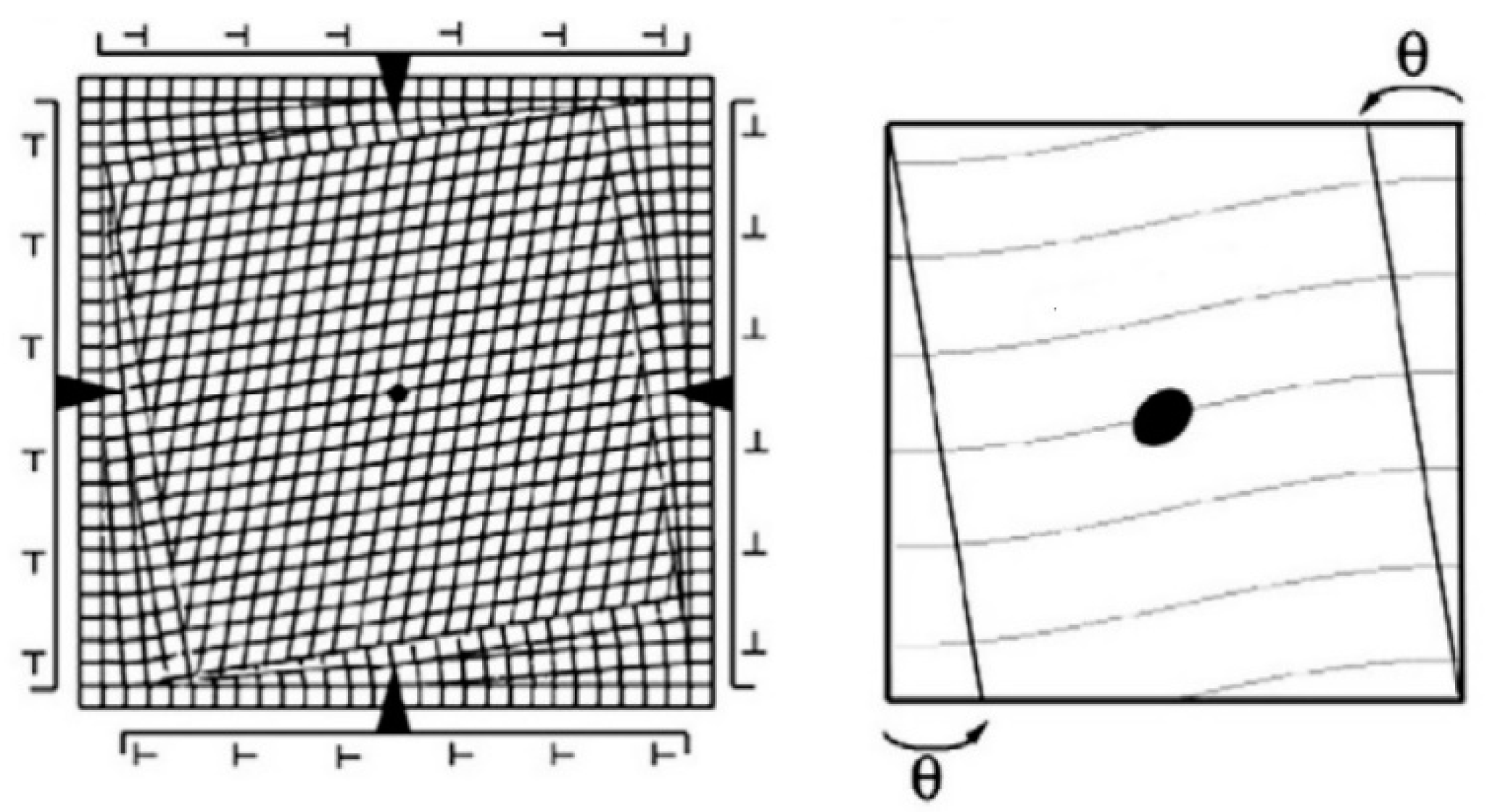
The concept of energy used in the modern version of PTMC is strange. It is assumed that “since a rigid rotation does not change the state of a crystal, it does not change the energy” [29]. This argument allows introducing all the extra rotation Q_ij or J_ijkl that are required to get compatibility conditions at the interfaces. It is usual in mechanics to decompose a strain matrix into a sum of a symmetric part and antisymmetric part if the strains are small, or into the product of a rotation and a symmetric matrix by polar decomposition if the strains are large. For a single crystal that is free to move instantaneously in its whole volume, one can keep only the symmetric part and ignore the antisymmetric part or the rotation because the rotation is free. However, in real materials the grains are not free to move; an accommodation between the martensite and the surrounding parent matrix is always required, even in the hypothetical case where the symmetric part is the identity and the deformation is a pure rotation. In addition, the transformation is never instantaneous because the martensite cannot go faster than the speed of sound. An accommodation between the transformed volume and the non-yet transformed volume is always needed in the transitory states, even in the hypothetical case where the austenite grain would not be blocked by the other grains and would be completely free. The elementary case of a pure “rotational transformation” is illustrated in Figure 3. In other words, the rotation part of a distortion can never be neglected. We are convinced that the gradients of the orientations observed in the pole figures of martensite in steels [43,47] result from the rotational parts of the lattice distortion that PTMC ignores by applying the “energy well” concept.

(iii)

The PTMC in its modern version confused some crystallographic notions. The term “correspondence variants” is used in place of “stretch variants”, as already explained in Ref. [54]. The variants are also not correctly treated from a mathematical point of view. For example, it is usually stated that the number of variants is the ratio of the number of symmetries of the daughter phase by that of the parent phase. This formula is in general incorrect because it does not specify the type of variants and does contain the related intersection group. The distortion, correspondence, or orientation variants are actually cosets based on intersection groups calculated with the distortion matrix F, the correspondence matrix C, or the orientation matrix T, respectively [54]. The coset decomposition dates from Janovec’s research about ferroelectric domains in 1972 [55,56] (see also [41]). The idea that the transformation is reversible because the number of symmetries of the daughter phase divides the number of symmetries of the parent phase results from the old concept of “symmetry breaking” that can be traced back to Landau [57], but it should be manipulated with a lot of rigor in crystallography. A simple cubic to tetragonal transformation is irreversible if the correspondence or orientation relationship is complex and if the lattice distortion has large values. The notion of group–subgroup relation has significance only if the type of relation (distortion, correspondence, or orientation) is specified.

1.3. EBSD/TKD, a Technique of Choice to Investigate NiTi Alloys

In order to see how the gap between the PTMC and our own approach to martensitic transformations could be filled, we decided to experimentally investigate the prototype of shape memory alloys: the NiTi alloys. Until now, all the characterization studies in this alloy have been performed by TEM or X-ray diffraction and interpreted with the PTMC. TEM gives information about the morphology, habit planes, and orientations with a sub-nanometer special resolution, but it lacks statistics because the observation areas are limited to the edges of the specimen. Classical X-ray diffraction allows collecting data on very large volumes, but the information about the interfaces and misorientations between the variants is missed. EBSD is a very good compromise between TEM and X-ray diffraction. Phase and orientation maps can be acquired on large surfaces (up to some mm²) with a resolution that can be better than 5 nm with field emission gun scanning (FEG) electron microscopes (SEM). Thanks to the recent development of Complementary Metal Oxide Semiconductor (CMOS) cameras [58], the acquisition speed can reach 3000 pixels/s; very large maps >1 million pixels are easily acquired with a very good angular resolution (<0.1°) and spatial resolution (<5 nm). TKD is exactly as EBSD, except that the sample is not anymore a bulk specimen tilted at 70° but a TEM lamella positioned very close to the SEM pole piece and tilted at −20°, such that the Kikuchi patterns are collected from the bottom surface of the specimen [59,60,61]. This technique took different names—t-EBSD, EFSD (Electron Forward-Scattering Diffraction), and more frequently TKD (Transmission Kikuchi Diffraction). A few years ago, we used this technique to map the lithiated (LiFePO₄)/unlithiated (FePO₄) regions in electrodes of lithium batteries during cycling [62]. The results were very conclusive, despite the fact that the lattice parameters of the two orthorhombic phases differ by less than 5%. This result reinforced our confidence in the capability of TKD to distinguish close phases, such as austenite and martensite in NiTi alloys.

2. Materials and Methods

Straight NiTi bars of 10 mm × 2 mm sections were used in this study. Their atomic composition measured by Energy Dispersive Spectrometry (EDS) is close to 50.0-50.0. The martensite start, martensite finish, austenite start, and austenite finish temperatures given for this alloy are M_s = 45 °C, M_f = 35 °C, A_s = 60 °C, and A_f = 90 °C. The shape memory effect was confirmed by manually deforming the bars into a U shape and checking that they come back to their initial straight shapes when they are put into hot water. The EBSD samples were prepared directly by electropolishing with an ATM machine using the A3 electrolyte from Struers at 20 V and 10 °C, or using a lab-made solution of 10% perchloric acid +30% butanol +60% methanol at 30 V. Some bars were also mechanically polished before electropolishing in order to get information far from the surface, and it was noticed that the electropolishing time had to be significantly increased to get good EBSD maps free of polishing artifacts. The TEM samples used for the TKD observations were prepared by mechanically polishing down to 100 μm and punching to obtain discs of 3 mm diameter. The discs were then electropolished at −15 °C with a dual-jet TenuPol electropolisher from Struers with the A3 electrolyte at 20 V, or with nitric 30% acid + 70% methanol solution at 40 V.

The EBSD and TKD maps were acquired with the CMOS Symmetry system processed with Aztec software (Oxford Instruments, UK). The camera is mounted on a Gemini450 SEM (Zeiss, Germany). Maps with a good spatial resolution/angular resolution/time per pixel could be obtained by working with a current of 15 nA and an accelerating voltage of 20 kV for EBSD and 30 kV for TKD.

Our software GenOVa [42] was used to simulate the orientation variants and their pole figures. Many different ORs (around fifteen) have been generated and compared with experience. The software ARPGE [39,40] was used to treat the experimental EBSD and TKD data, and more particularly to:

(i)

Reconstruct the prior parent B2 parent grains. The reconstruction uses the groupoid composition table generated by GenOVa. The retained B2 phase is ignored when it exists. Since the fraction of the indexed B19′ is quite low, a numerical dilatation was systematically performed in order to create a contact between the martensite plates.

(ii)

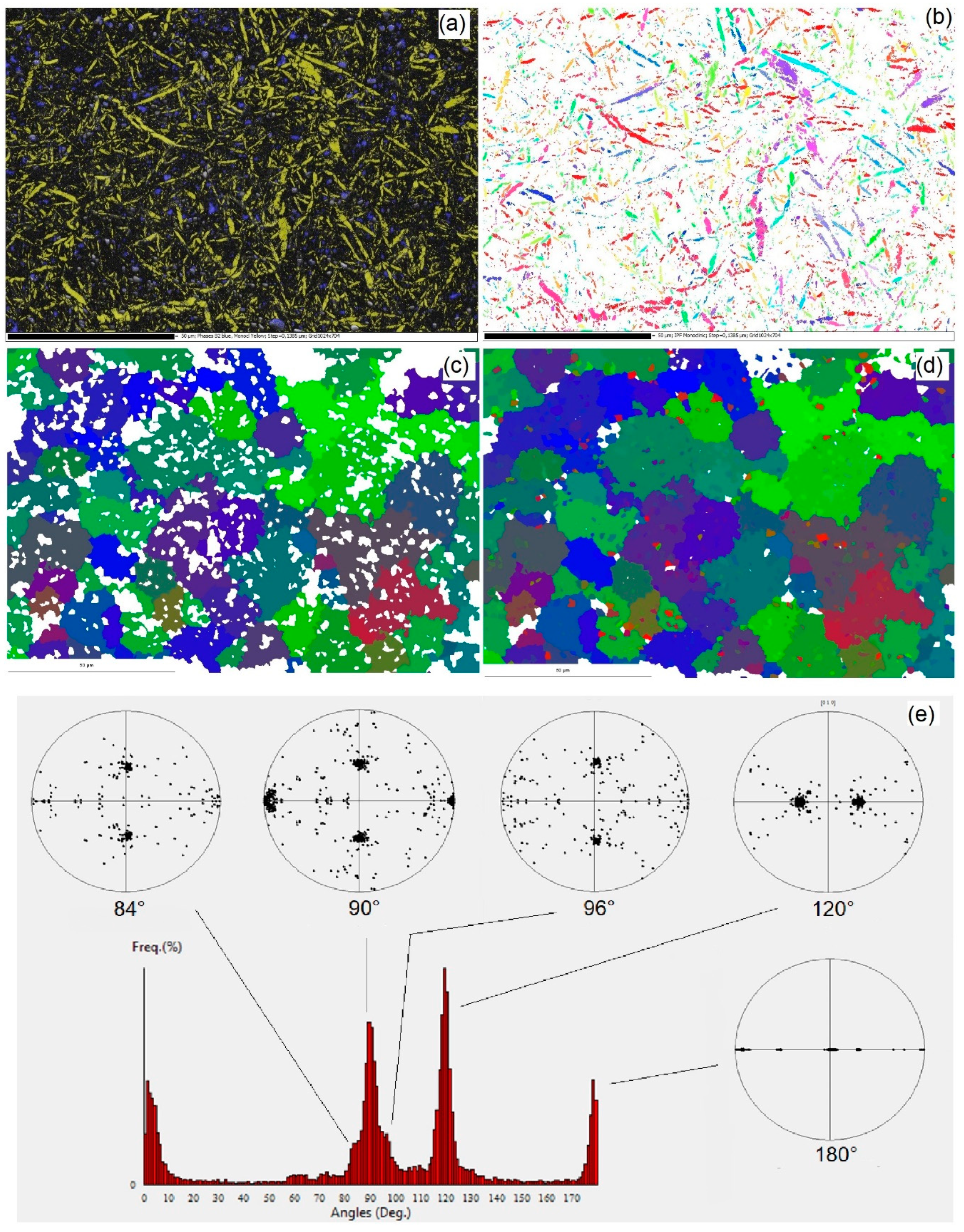
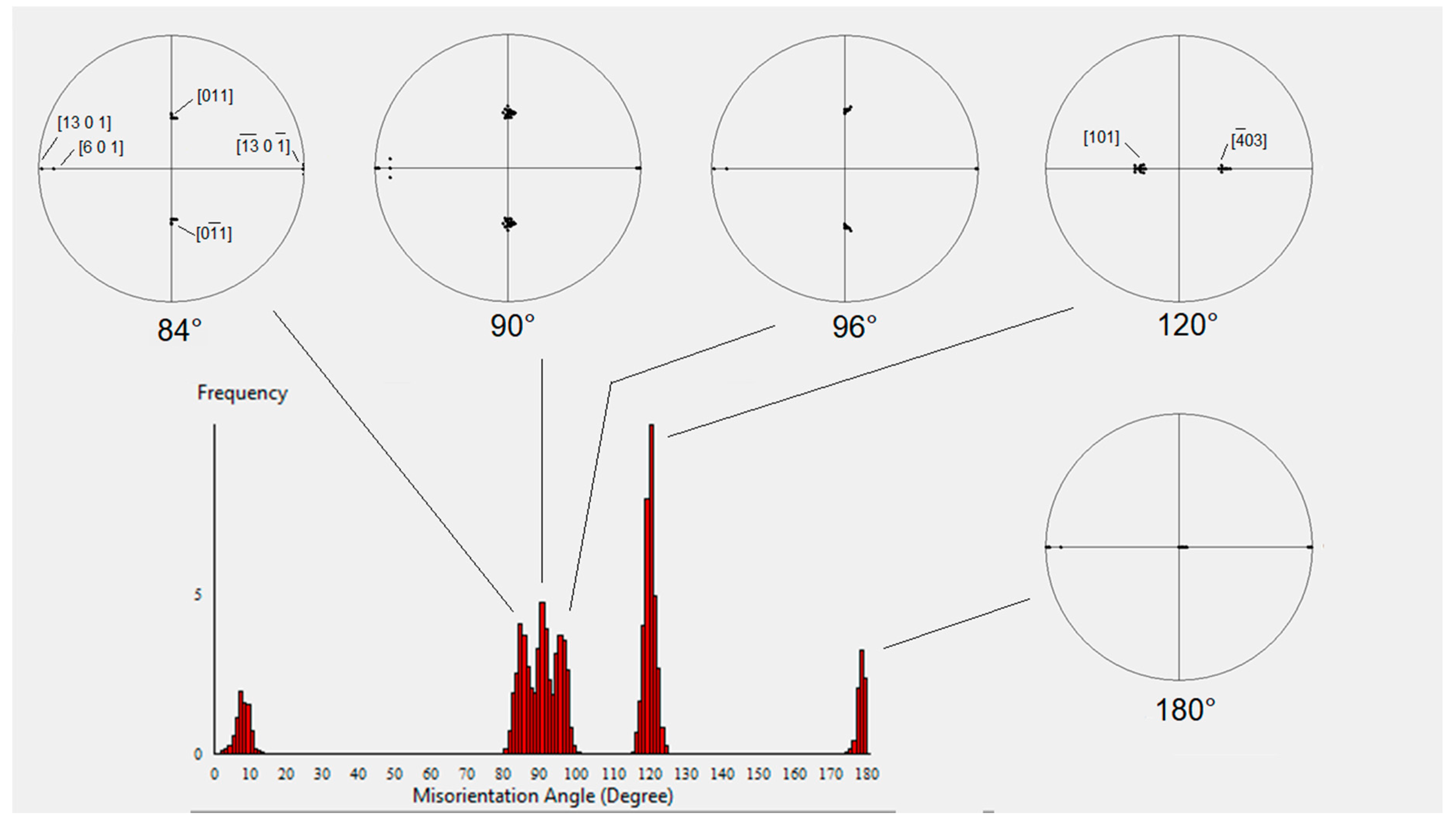
Plot the misorientations between the B19′ martensite inside all the prior parent B2 grains. The rotation axes corresponding to the peaks in the disorientation histograms are reported in pole figures. This function exists in Channel5 but is not very practical.

(iii)

Plot the traces in the EBSD and TKD maps of some predicted planes. This function does not exist in Channel5 but is very useful in verifying whether or not a habit plane or junction plane expected by the theory fits with the experiments.

For the calculations, we used the same lattice parameters as reported for NiTi alloys in the PTMC studies—i.e., a = 3.015 Å for B2; a = 2.89 Å, b = 4.12 Å, c = 4.62 Å, and β = 96.8° for B19′. We would like to remind the reader of some crystallographic notions that will be useful. In a monoclinic structure, the directions a and c are normal to b. In the B19′ phase, the normal to the plane (010) is also the direction [010], but the plane (100) has for normal the direction ~[13,0,1], and the plane (011) has for normal the direction ~[3,0,16]. Due to the mirror (010)_B19′ and (180°, b) symmetries of the B19′ structure, there is an equivalency relation between the directions [u,v,w] ≡ [u,$\overline{v}$,w], and also between the planes (h,k,l) ≡ (h,$\overline{k}$,l). Combined with the inversion symmetry, there is also an equivalency between the directions [$\overline{u}$,v,w] ≡ [u,v,$\overline{w}$], and between the planes ($\overline{h}$,k,l) ≡ (h,k,$\overline{l}$). One should remember that the direction [u,v,w] is not equivalent to [u,v,$\overline{w}$], and the plane ($h,$k,l) is not equivalent to (h,k,$\overline{l}$).

3. EBSD Results

More than fifteen EBSD maps have been acquired at medium magnifications (between ×700 and 10k). The indexation rate is low, often between 40% and 60%, but the maps are not noisy in the sense that they exhibit large and well indexed B19′ lenticular martensite surrounded by a non-indexed “matrix” probably composed of martensite that is too fine to be indexed. In most of the maps, some small islands with a cubic structure are visible. When they have a facetted morphology, they are probably cubic precipitates misindexed as B2 phase, but in in some maps (not shown here) the zones indexed as B2 are really B2, because they form large equiaxed grains in a volume fraction that is far greater than that of B19′ martensite, and they cannot be confused with precipitates. The reason of the presence of large volumes of B2 phase in some specimens is not yet fully understood, but we noticed that electropolishing some deformed samples can lead to a “memory effect” associated with the B19′→B2 transformation. Thus, we think that the B2 phase, when it is visible and unambiguous, is not a “retained” (untransformed) B2 but a new B2 generated by the reverse B19′→B2 transformation. Consequently, the B2 islands will be called “reversed” B2. In none of the EBSD maps could the “twins” inside the B19′ martensite be imaged. As will be shown in Section 4, they are present, but their size and density do not allow EBSD to capture them.

Two EBSD maps acquired at ×2k and ×3k magnifications are shown in Figure 4a,b and Figure 5a,b (the parts c, d, and e will be discussed later).

The convention used to plot the rotation axes in Figure 4e and Figure 5e in a XY stereographic projection is b_B19′//Y and c_B19′//Z, as described in Figure 6. We draw the reader’s attention to the fact that, since β > 90°, the axis a_B19′ should be represented by its opposite—a_B19′—and its projection is not exactly on the external (XY) circle.

The pole figures of the B19′ martensite and reversed B2 in selected subsets of the EBSD maps allowed us to determine the ORs between the two phases. Different directions and planes were plotted in order to find by overlapping which directions or planes of B2 are parallel to those of B19′ martensite. As shown in Figure 7, some unambiguous parallelisms between planes and directions exist: {100}_B19′//{100}_B2, <100>_B19′//<100>_B2, {010}_B19′//{110}_B2, <110>_B19′//<111>_B2, <101>_B19′//<111>_B2, <10$\overline{1}$>_B19′//<111>_B2.

These parallelisms can be interpreted by distinct ORs that are:

• OR A: (010)_B19′//(110)_B2 and (100)_B19′//(001)_B2 ⇔ (010)_B19′//(110)_B2 and [001]_B19′//[$\overline{1}$10]_B2;
• OR C: (010)_B19′//(110)_B2 and (001)_B19′//($\overline{1}$10)_B2 ⇔ (010)_B19′//(110)_B2 and [100]_B19′//[001]_B2;
• OR AQ: (010)B19′//(110)B2 and [101]_B19′//[$\overline{1}$11]_B2;
• OR CQ: (010)_B19′//(110)_B2 and [10$\overline{1}$]_B19′//[$\overline{1}$1$\overline{1}$]_B2.

Another OR could also be identified from the experimental pole figures shown in Figure 8. It is:

• OR I: (11$\overline{1}$)_B19′//(101)_B2 and [011]_B19′//[$010$]_B2.

The OR I is not as clear as the previous ones because the spots are quite spread out, but it is very important to simulate the disorientation histograms, as detailed in the following sections. The names A and C were given according to the plane of the martensite that is parallel to a low-index crystallographic plane of the B2 phase. The names AQ and CQ come from the fact that they are quasi-A and quasi-C, respectively—i.e., they differ from each other by a few degrees, as shown in Figure 9a,b. The name OR I is given because it is like an intermediate between the two groups OR A/AQ and OR C/CQ, as shown in Figure 9c. The number of orientation variants for the ORs A, AQ, C, or CQ is 12, and that of OR I is 24. Note that the OR A is exactly that represented by Otsuka and Ren [13,38] and reported in Figure 1.

The strongest OR among all these ORs in the pole figures is the OR A or AQ (they are difficult to discriminate). The OR AQ was thus used to reconstruct the prior parent B2 grains with our software ARPGE. The reconstructed grains for the maps of Figure 4b and Figure 5b are given in Figure 4c and Figure 5c, respectively. Their orientations fit quite well with those of the existing “reversed” B2, as shown in the IPFz maps of Figure 5d. After the reconstruction, the histogram of the disorientations of the B19′ martensite plates contained in each of the prior parent B2 grains are plotted in Figure 4e and Figure 5e. They exhibit five peaks at 84°, 90°, 96°, 120°, and 180°. ARPGE permits us to automatically plot on a stereographic projection the B19′ rotation axes that correspond to these angles. They are distributed around specific poles, as shown in Figure 4e and Figure 5e. All the variants of the five ORs—A, AQ, C, CQ, and I—were created with GenOVa [41,42]. For each OR, the specific misorientations between them are calculated. They are called “operators” [41]. An operator is expressed by a set of equivalent rotations, and it is usual (even if arbitrary) to choose the rotation with the smallest angle called “disorientation”. The disorientation operators associated with the five ORs are given in Figure 10.

It can be noticed that only the OR I gives angles that deviate from 90° (84° and 96°) or from 120° (116°). All the operators are however insufficient to simulate in detail the experimental histograms of Figure 4e and Figure 5e. We thus wrote an additional computer program that calculates the misorientations between the variants of the different ORs in the list {A, AQ, C, CQ, I, and A-C}. By the term “A-C”, we mean a continuum of orientations between the rotation A and C, as described in Figure 11. This continuum has been modeled by five intermediate ORs between A and C separated by 1°. The idea of introducing the continuum comes from our experience with steels and the continuums that exist between the KS, NW, and Pitsch ORs [47].

Taking into account all the variants of all the ORs and all their misorientations, we can now simulate the disorientation histogram and the stereographic projection of the rotation axes corresponding to the histogram peaks, as shown in Figure 12.

The simulations now fit very well with the experimental results obtained in Figure 4e and Figure 5e. All the orientation relationships, and particularly OR I and the continuum A-C, brought an important contribution to the histograms and to the distributions of the rotation axes. In the supplementary material A of our work on martensite in steels [47], we noticed that the continuum of OR can be missed if the EBSD step size is too large or if the scanning resolution is not sufficient. Could it be the same for NiTi alloys? Does the continuum we inferred to simulate the EBSD disorientation histograms really exist? In order to check this point, we decided to prepare TEM lamellae and perform TKD. The increase in the spatial resolution will be also useful to reveal the “twins”. These twins inside the B19′ martensite plates remained invisible in EBSD because they are too small and their density too low. They are usually studied by TEM (see Section 1).

4. TKD Results

The quality of a TKD map greatly depends on the quality of the TEM lamella, which should be thin and homogeneous over a large area, even if it is true that the large dynamic range of the CMOS EBSD camera really helps to increase the tolerance to the change in intensity due to thickness gradients. We acquired more than 15 TKD maps of five TEM lamellae close to the holes made by electropolishing. The indexation rate is better than EBSD; it is often between 65% and 85%. One of the TKD maps is shown in Figure 13. The long and individual plate shapes of the B19′ martensite imaged by EBSD are not visible anymore because of the smaller field of view, but the increase in magnification (×10 in comparison with EBSD) now makes the “twins” clearly visible. We treated the TKD maps exactly as the EBSD maps. The prior parent B2 grains were reconstructed with ARPGE; they are shown without and with the “reversed” B2 in Figure 13c,d, respectively. The disorientation histogram and associated rotation axes are plotted in Figure 13e. The histogram is similar to those obtained by EBSD; however, the peak at 90° is now less intense than those at 84° and 96°, and the peak at 120° is asymmetric and shifted toward 115°. The rotation axes are clustered around the same poles as for EBSD, with a lower spreading, probably because of the lowest statistics on the number of grains mapped by TKD. The simulations made in Figure 12 also fit well with the experimental TKD disorientation histogram.

The pole figures of the {100}, {010}, and {001} planes of the B19′ martensite are shown in Figure 14. The pole figures of other planes and directions are shown in Figure 15. With only the 12 + 12 = 24 variants generated by the ORs A and C, the {100} and <100> EBSD pole figures exhibit only three groups of five spots forming the symbol five in a dice, as can be noticed in the EBSD <100> pole figure of Figure 7. Now, thanks to the TKD resolution, the {100} and <100> pole figures of the B19′ martensite clearly exhibit the continuum of rotations expected from our EBSD analysis. The A-C continuum makes that the “dice-5” feature becomes a “four-fold cross”, as shown in the left column of Figure 14a and Figure 15a. The experimental pole figures in Figure 14a and Figure 15a are well simulated with all the variants generated by the ORs A, AQ, C, CQ, I and the A-C continuum, as shown in Figure 14b and Figure 15b. The good fit can be checked by overlapping (Figure 14c and Figure 15c), even if some tiny details of the shapes of the features are not yet exactly reproduced.

These results demonstrate that TKD brings additional information to EBSD. The intricate structures of the B19′ domains (“twins”) become clearly visible. The resolution is not as good as that of conventional TEM, but is sufficient to extract relevant crystallographic information about the orientations of the domains and their junction planes. Surprisingly, the 90° peak in the EBSD disorientation histograms nearly disappears in TKD, and the 120° peak is shifted toward 115°. It seems that the crystallographic information depends in its details on the length scale of the observation, whether that of EBSD or that of TKD. We will try to explain why in the next section.

5. Crystallographic Analysis

The EBSD and TKD experimental results reported in the two previous sections are now analyzed according to the approach explained in Section 1.2. If the reader would like to develop another interpretation, for example based on the PTMC, the data are available on simple demand to the author.

5.1. The Natural OR

As mentioned in the introduction, our experience of martensitic transformation in steels and titanium alloys leads us to conclude that there should exist a “natural” OR, and that the other ORs derive from this natural OR. The “natural” OR establishes a parallelism of the dense planes and dense directions of the parent and daughter phases. In the case of NiTi, the dense planes of the B2 phase are {110}, and the dense directions are <111>. What are the dense planes and directions of B19′ martensite? Let us consider again Otsuka and Ren’s schematic representation of the B2–B19′ transformation in Figure 1. Some Ni atoms shuffle (i.e., they do not follow the same trajectories as the nodes of the B19 supercell), but the striking point is that some of them remain in the plane (110)_B2 that becomes (010)_B19′. In addition, the direction [$\overline{1}$11]_B2 has a length of 5.22 Å, and among all the possible reticular directions of B19′, the direction [101]_B19′ has the closest length to it (5.15 Å). Therefore, according to the idea that the natural OR is that one that establishes a parallelism between the dense(est) planes and directions, it appears that OR AQ, for which (010)_B19′//(110)_B2 and [101]_B19′//[$\overline{1}$11]_B2, should be the “natural” OR of B19′ martensite. This theoretical result is in good agreement with the fact that OR AQ (or A) is the predominant OR observed by EBSD (Section 3).

Note: We take the opportunity of this paper to propose a possible explanation for the strange observation made by Gu et al. [31]. They observed that for many cubic-orthorhombic transformations in Ti-based shape memory alloys, when the eigenvalues ${\lambda }_1\le 1$ and ${\lambda }_3\ge 1$ of the stretch matrix are plotted on a graph reproduced in Figure 16, they “fall closely on a straight line in this plot, a fact which is not understood”. We think it possible that these two values are actually linked by the existence of an invariant dense direction, which would be the diagonal of the rectangle formed by the eigenvectors associated with ${\lambda }_1$ and ${\lambda }_3$. It would mean that, for all these transformations, the values are linked by the relation ${\lambda }_1^2+{\lambda }_3^2=2$. As ${\lambda }_1$ and ${\lambda }_3$ are close to 1, the curve representing the relation $y=\sqrt{2-x^2}$ between ${\lambda }_1$ and ${\lambda }_3$ is nearly a line. We reported it in a green dash on Figure 16, and it fits well with the experimental points.

5.2. The Martensite Habit Planes

If AQ is the natural OR, one should be able to predict the habit planes from the associated distortion matrix. As explained in Section 1.2, this plane does not need to be necessarily fully invariant, but it should be at least unrotated by the distortion [48]—i.e., it should be an eigenvector of the distortion matrix expressed in the reciprocal space ${\mathbf{F}}^{*}={\mathbf{F}}^{-\mathrm{t}}$. Combining two variants can probably make it fully invariant, as in high-carbon steels [50], but we think that the condition is not mandatory because elastic or plastic accommodation inside the plane is possible. Such intraplanar accommodation is actually as relevant as the accommodation required at the austenite/martensite interfaces perpendicular to the habit planes. All the ORs in the list {A, AQ, C, CQ, I} share the same correspondence matrix $\mathbf{C}$. By considering Figure 1, we can see that the direction a_B19′ comes from [001]_B2, and the directions bB19′ and cB19′ from [110]_B2 and [1$\overline{1}$0]_B2, respectively. The slight misorientations between the ORs A, AQ, C, CQ, and I change nothing to the correspondence. For all of them, the correspondence matrix is thus (see [54] if necessary):

$${\mathbf{C}}_{}^{\mathrm{B}2\to \mathrm{B}19\prime }=\left[\begin{array}{ccc}0& 1& -1\\ 0& 1& 1\\ 1& 0& 0\end{array}\right].$$

(1)

We decided to calculate the orientation matrix $\mathbf{T}$ and the distortion matrix $\mathbf{F}$ for each of the ORs reported in the list {A, AQ, C, CQ, I}. If the natural OR is really AQ, it should give us the correct habit plane, and the other ORs should not (except by coincidence).

Let us start with the OR A represented in Figure 1. In order to determine the orientation matrix, we use the ideal orthorhombic B19 supercell that is transformed into the B19′ monoclinic cell only by opening the angle β from 90° to β_B19′ = 96.8°. We write the orientation matrix ${\mathbf{T}}_A^{\mathrm{B}2\to \mathrm{B}19\prime }$ as the product of the coordinate transformation matrices $\left[{\mathbf{ℬ}}_{}^{\mathrm{B}2}\to {\mathbf{ℬ}}_{}^{\mathrm{B}19}\right]\left[{\mathbf{ℬ}}_{}^{\mathrm{B}19}\to {\mathbf{ℬ}}_{}^{\mathrm{B}19\prime }\right],$ where A stands for the OR A. The first matrix is:

$$\left[{\mathbf{ℬ}}_{}^{\mathrm{B}2}\to {\mathbf{ℬ}}_{}^{\mathrm{B}19}\right]=\left[\begin{array}{ccc}0& \frac{1}{\sqrt{2}}\frac{b_{B19\prime }}{{\mathrm{a}}_{B2}}& \frac{-1}{\sqrt{2}}\frac{c_{B19\prime }}{{\mathrm{a}}_{B2}}\\ 0& \frac{1}{\sqrt{2}}\frac{b_{B19\prime }}{{\mathrm{a}}_{B2}}& \frac{1}{\sqrt{2}}\frac{c_{B19\prime }}{{\mathrm{a}}_{B2}}\\ \frac{a_{B19\prime }}{{\mathrm{a}}_{B2}}& 0& 0\end{array}\right],$$

The second matrix is:

$$\left[{\mathbf{ℬ}}_{}^{\mathrm{B}19}\to {\mathbf{ℬ}}_{}^{\mathrm{B}19\prime }\right]=\left[\begin{array}{ccc}Sin\left({\beta }_{B19\prime }\right)& 0& 0\\ 0& 1& 0\\ \mathrm{Cos}\left({\beta }_{B19\prime }\right)& 0& 1\end{array}\right].$$

From the calculation of these matrices, the orientation matrix is thus:

$${\mathbf{T}}_A^{\mathrm{B}2\to \mathrm{B}19\prime }=\left[\begin{array}{ccc}0.128& 0.966& -1.084\\ -0.128& 0.966& 1.0834\\ 0.951& 0& 0\end{array}\right].$$

The fundamental equation that links the orientation, correspondence, and distortion matrices [54] is:

$${\mathbf{C}}_{}^{\mathrm{B}19\prime \to \mathrm{B}2}={\mathbf{T}}_{}^{\mathrm{B}19\prime \to \mathrm{B}2}{\mathbf{F}}_{}^{\mathrm{B}2},$$

(2)

where ${\mathbf{C}}_{}^{\mathrm{B}19\prime \to \mathrm{B}2}={\left({\mathbf{C}}_{}^{\mathrm{B}2\to \mathrm{B}19\prime }\right)}^{-1}$ and ${\mathbf{T}}_{}^{\mathrm{B}19\prime \to \mathrm{B}2}={\left({\mathbf{T}}_{}^{\mathrm{B}2\to \mathrm{B}19\prime }\right)}^{-1}$. It is used to directly calculate the distortion matrix in the B2 crystallographic basis.

$${\mathbf{F}}_A^{\mathrm{B}2}=\left[\begin{array}{ccc}1.025& -0.059& 0.128\\ -0.059& 1.025& -0.128\\ 0& 0& 0.951\end{array}\right].$$

In order to calculate the distortion matrices of the other ORs, we applied a numerical method already detailed in the supplementary materials of Ref. [63]. Let us explain it by showing how to deduce ${\mathbf{F}}_{AQ}^{\mathrm{B}2}$ from ${\mathbf{F}}_A^{\mathrm{B}2}$. The distortion ${\mathbf{F}}_{AQ}^{\mathrm{B}2}$ should leave the direction u = [$\overline{1}$11]_B2 unrotated, whereas this is not the case for ${\mathbf{F}}_A^{\mathrm{B}2}$. The angle of rotation α = ($\mathbf{u}$, ${\mathbf{F}}_A^{\mathrm{B}2}\mathbf{u}$) is calculated, and the rotation matrix R of angle α and axis ($\mathbf{u}\bigwedge {\mathbf{F}}_A^{\mathrm{B}2}\mathbf{u}$) is determined. The distortion related to the orientation AQ is thus simply ${\mathbf{F}}_{AQ}^{\mathrm{B}2}$ = ${\mathbf{R}}^{-1}{\mathbf{F}}_A^{\mathrm{B}2}$. The same method is applied to compensate the rotation of a plane, if necessary. In that case, the matrices should be expressed in the reciprocal space before coming back to the direct space. Once the distortion matrices are calculated, the orientation matrix is deduced from the relation (2). The rounded values of the distortion matrices calculated with Mathematica are given in

Table 1. Distortion matrices ${\mathbf{F}}_{OR}^{\mathrm{B}2}$ associated with the different ORs determined in Section 3. The eigenvectors of ${\left({\mathbf{F}}_{}^{\mathrm{B}2}\right)}^{*}$ are the planes unrotated by the distortion and are thus candidates to be the martensite habit plane. They are calculated on the B2 basis and given in the second column. The orientation matrices ${\mathbf{T}}_{OR}^{\mathrm{B}2\to \mathrm{B}19\prime }$ can be calculated from the correspondence matrix (1) and the fundamental Equation (2).

OR	Distortion Matrix ${\mathbf{F}}_{}^{\mathbf{B}\mathbf{2}}$	Eigenvectors of ${\left({\mathbf{F}}_{}^{\mathbf{B}\mathbf{2}}\right)}^{*}={\left({\mathbf{F}}_{}^{\mathbf{B}\mathbf{2}}\right)}^{-\mathbf{t}}$
A	${\mathbf{F}}_A^{\mathrm{B}2}=\left[\begin{array}{ccc}1.025& -0.059& 0.128\\ -0.059& 1.025& -0.128\\ 0& 0& 0.951\end{array}\right]$	$\left\{0,0,1\right\}$, $\left\{1,1,0\right\},\left\{0.417,-0.417,0.807\right\}$
AQ	${\mathbf{F}}_{AQ}^{\mathrm{B}2}=\left[\begin{array}{ccc}1.025& -0.059& 0.130\\ -0.059& 1.025& -0.130\\ -0.0016& 0.0016& 0.951\end{array}\right]$	$\left\{0.012,-0.012,0.999\right\},\left\{1,1,0\right\},\left\{\mathbf{1},-\mathbf{1},\mathbf{2}\right\}$
C	${\mathbf{F}}_C^{\mathrm{B}2}=\left[\begin{array}{ccc}1.021& -0.055& 0\\ -0.055& 1.021& 0\\ 0.057& -0.057& 0.958\end{array}\right]$	$\left\{-0.397,0.397,0.827\right\},\left\{1,1,0\right\},\left\{-1,1,0\right\}$
CQ	${\mathbf{F}}_{CQ}^{\mathrm{B}2}=\left[\begin{array}{ccc}1.022& -0.056& 0.054\\ -0.056& 1.022& -0.054\\ 0.083& -0.083& 0.966\end{array}\right]$	$\left\{-1,1,2\right\},\left\{1,1,0\right\},\left\{0.642,-0.642,0.420\right\}$
I	${\mathbf{F}}_I^{\mathrm{B}2}=\left[\begin{array}{ccc}1.020& 0& 0.0939\\ -0.118& 1.0268& -0.135\\ 0.0287& 0& 0.954\end{array}\right]$	$\left\{0.293,0,-0.956\right\},\left\{0.713,0.125,0.690\right\},\left\{1,0,1\right\}$

.

For each of the ORs in the table, the three eigenvectors of ${\left({\mathbf{F}}_{OR}^{\mathrm{B}2}\right)}^{*}$ are candidates to be the martensite habit plane. They were then expressed on the B19′ basis, thanks to the inverse of the coordinate transformation matrix ${\mathbf{T}}_{OR}^{\mathrm{B}2\to \mathrm{B}19\prime }$, and their traces were plotted with ARPGE in all the B19′ grains of the EBSD maps. The best agreement was obtained for the OR AQ and for the plane ${\mathbf{g}}_{\mathrm{B}2}$ = (1$\overline{1}$2)_B2—that is, the plane ${\mathbf{g}}_{\mathrm{B}19\prime }$ = (10$\overline{1}$)_B19′ by orientation ${\left({\mathbf{T}}_{AQ}^{\mathrm{B}19\prime \to \mathrm{B}2}\right)}^{*}{\mathbf{g}}_{\mathrm{B}2}$ and by correspondence ${\left({\mathbf{C}}_{}^{\mathrm{B}19\prime \to \mathrm{B}2}\right)}^{*}{\mathbf{g}}_{\mathrm{B}2}$, as shown in Figure 17. Please note that for the OR CQ, the plane ($\overline{1}1$2)_B2 becomes the plane ${\mathbf{g}}_{\mathrm{B}19\prime }$ = (10$1$)_B19′, which is not equivalent to (10$\overline{1}$)_B19′, and this plane does not fit at all with the EBSD maps. Actually, none of all the other planes deduced from Table 1 fit with the experimental data, except the plane ${\left\{0.417,-0.417,0.807\right\}}_{B2}$ of the OR A, because it also corresponds to a plane very close to (10$\overline{1}$)_B19′.

As detailed in the introduction, the habit planes predicted by the PTMC (i.e., the one among the four solutions of the PTMC equations that is the closest the experience) is (0.215,0.405,0.888)_B2, whereas the experimentally measured habit planes reported in the literature is close to (0.39,0.48,0.78)_B2 with a spreading of ±4°. We transformed the plane (0.39,0.48,0.78)_B2 into B19′ planes according to the different ORs, and we plotted their traces on the EBSD maps. The traces are also close to the ones plotted in Figure 17, but the agreement seems less satisfactory. Even if we consider that the habit planes are (0.39,0.48,0.78)_B2, as reported in literature, one should note that the habit plane (1$\overline{1}$2)_B2 chosen among the three solutions in the set of eigenvectors of ${\left({\mathbf{F}}_{AQ}^{\mathrm{B}2}\right)}^{*}$ is in better agreement with it than the (0.215,0.405,0.888)_B2 plane calculated by PTMC. Indeed, the angle between the plane (0.39, 0.48, 0.78)_B2 and the plane (112)_B2 is 4.7°, whereas it is 12.6° with (0.215,0.405,0.888)_B2.

5.3. The Closing-Gap ORs and the Continuums of Orientation Relationship

The continuum of ORs inferred from the EBSD analyses was confirmed by TKD. The EBSD maps gave information on the average orientations and misorientations and ignored the details and the fine structure of “twins” present in some martensite. The TKD maps revealed the presence of the twins at a higher magnification and simultaneously confirmed the continuums of orientations, as illustrated by the change in the “dice-5 feature” of the <100>_B19′ EBSD pole figures into the “four-fold cross” of the TKD pole figures. The “twins” and the continuum of orientations seems to be correlated. Let us explain why with our model.

First, we would like to show how it differs from the PTMC. From its beginning, the PTMC considers as a fundamental point the compatibility condition between the variants and the austenite and between the variants themselves. This compatibility is indeed required, because no holes or cracks could ever be observed at the interfaces. However, as shown in the introduction, the PTMC uses “free” rotations to reach the compatibility conditions, such as the free rotations Q_ij required to obtain the compatibility between the pairs of variants (i,j). Let us explain again with the 2D example of the square (γ) to parallelogram (α) transformation of Figure 18 how the PTMC establishes its compatibility criterion. In Figure 18a, the junction plane between two stretch variants (i,j) noted by the normal m is inherited by lattice distortion from an austenite plane n that is not necessary parallel to m, thanks to the rotation Q_ij that provides a degree of freedom. The martensite composite (“habit plane variant”) is made of the two variants in a proportion x and (1 − x), such that a plane of the austenite is also compatible with a plane of the composite (the habit plane), as shown in Figure 18b. The two variants are orientated as if both were linked by a simple shear (Figure 18c)—that is why they are called “twins”. The PTMC uses the exact values of the lattice parameters to calculate the stretch distortions.

More rotational degrees of freedom are introduced with the matrices J_ik for the compatibility between the major variants i and k of two martensite products (i,j) and (k,l) [34], and with J_ijkl for the compatibility between the habit plane variants (i,j) and (k,l) [37]. One could imagine even more rotations by considering larger assemblies of variants. One could probably see a link between them and the continuums of orientations observed by TKD (Section 4), but the calculations of the matrices Q_ij, J_ij, J_ijkl, etc. seems really complex, and we doubt that they would fit the observations.

The PTMC works locally on each pair of stretch variants, but it does not capture the structure of the variants as a whole. Our approach also uses the fact that a compatibility should exist between the distortion variants, but it tries to reach the best comprise between the local compatibility required between the individual variants and the global integrity that should be maintained in the whole intricate structure. As explained in the introduction, the continuums of ORs were already identified in martensite in steels and in deformation twins in magnesium, and we already showed that they are a consequence of the distortion itself. The present experimental results confirms this approach for the NiTi alloys and permits us to complete it. In our approach, there is a “natural” OR—here, AQ—and this OR is not based on the exact metrics of the phases, since the dense directions and dense planes do not have exactly the same length in the parent and daughter phases. Now, we interpret the additional ORs—A, C, CQ, and I—as intermediate ORs required to maintain the compatibility between the AQ distortion variants. They are like “closing-gap” ORs generated by the distortion field between two AQ variants, and they derive from the natural OR by a continuum of orientations. Let us explain this idea with the simple 2D example of square (γ) to parallelogram (α) transformation. If we consider that the natural OR is [1,0]_γ//[1,0]_α and (0,1)_γ//(0,1)_α, simple geometry or coset decomposition [54] shows that there are four distortion variants, as represented in Figure 19a. Clearly, there is no plane (actually direction in 2D) that is compatible between the variants (α_i, α_j) whatever the pair. However, let us consider the pair (α₁, α₃) in Figure 19b; besides the planes (0,1)_α the two variants in this pair have another common plane by correspondence—that is, the plane (1,0)_α (which is also the direction b_α in 2D). This plane is inherited from the austenite plane $m_y^{\gamma }$ for both of them, but it is rotated clockwise by the distortion of α₁ and anticlockwise by the distortion of α₃, which means that they are not parallel anymore once the distortion is finished. Thus, a “natural” compatibility between the variants α₁ and α₃ is the one that existed at the early stage of the distortion process when both of them shared the plane $m_y^{\gamma }$. The variants are linked by the correspondence $m_y^{\gamma }\to {\left(1,0\right)}_{\alpha 1}$ and $m_y^{\gamma }\to {\left(1,0\right)}_{\alpha 3}$. We make the hypothesis that the link is not totally lost and the two variants remain joined by a continuum of distortion such that the plane ${\left(1,0\right)}_{\alpha 1}$ is continuously rotated counter-clockwise and ${\left(1,0\right)}_{\alpha 3}$ is continuously rotated clockwise to come back parallel to $m_y^{\gamma }$. This gradient of lattice distortion is nothing else than a kind of elastic or plastic heritage of the initial mechanism of transformation. It induces a continuum of ORs initiated from the natural OR by a back-stress effect in martensite, such as that schematized in Figure 2 (see [43]), or by the fact that martensite continues to grow in a rotated austenite matrix [47]. The compatibility is thus such that ${\left(1,0\right)}_{\alpha 1}$//${\left(1,0\right)}_{\alpha 3}$//${\left(1,0\right)}_{\gamma }$, which appears as a secondary OR different from the natural OR. Similarly, the distortion variants α₁ and α₂ are linked by the correspondence $m_{xy}^{\gamma }$→${\left(\overline{1},1\right)}_{\alpha 1}$ and $m_{xy}^{\gamma }$→${\left(\overline{1},1\right)}_{\alpha 2}$, which induces a secondary OR ${\left(\overline{1},1\right)}_{\alpha 1}$//${\left(\overline{1},1\right)}_{\alpha 2}$//${\left(\overline{1},1\right)}_{\gamma }$, as shown in Figure 19c.

Consequently, contrarily to the PTMC, we assume that the compatibility between two variants i and j is obtained along a prior austenite symmetry element that is “lost” by the distortion but preserved by correspondence. Let us give a global picture of this model and explain how it can be used to determine the habit planes and junction planes. We assume that there exist a unique correspondence encoded by the matrix C, a unique OR (the natural OR) encoded by the matrix T, and thus a unique distortion given by the matrix F [54]. The distortion variants are defined from the left-cosets of type g${ℍ}_{\mathrm{F}}^{\gamma }$, where ${ℍ}_{\mathrm{F}}^{\gamma }$ is the subgroup of ${\mathbb{G}}^{\gamma }$ (the point group of the parent phase) formed by the geometrical symmetries left invariant by the distortion F. The elements g are the symmetry matrices of the point group of austenite. The coset g₁${ℍ}_{\mathrm{F}}^{\gamma }$ = ${ℍ}_{\mathrm{F}}^{\gamma }$ (g₁ = identity matrix) defines the distortion variant 1, g₂${ℍ}_{\mathrm{F}}^{\gamma }$ the variant 2, g₃${ℍ}_{\mathrm{F}}^{\gamma }$ the variant 3, etc. The elements of g_i${ℍ}_{\mathrm{F}}^{\gamma }$ are the symmetries g_i that are preserved by the distortion of the variant i. Two distortion variants defined from the cosets g_i${ℍ}_{\mathrm{F}}^{\gamma }$ and g_j${ℍ}_{\mathrm{F}}^{\gamma }$, i.e., F_i $\in$ g_i${ℍ}_{\mathrm{F}}^{\gamma }$F and F_j $\in$ g_j${ℍ}_{\mathrm{F}}^{\gamma }$F have no symmetry in common (because the cosets are disjoint), but they can share a common unrotated plane, i.e., a common eigenvector of their reciprocal distortion matrix). This will be the habit plane of the martensite composite (habit plane variant). In the example of Figure 19, the habit plane of the habit plane variant (1,3) is the plane ${\left(0,1\right)}_{\alpha 1}$//${\left(0,1\right)}_{\alpha 3}$//${\left(0,1\right)}_{\gamma }$. We point out here that this plane can also be the habit plane of the individual variant 1, or of the individual variant 3, because it is unrotated by their distortion. Independently of the habit plane, the compatibility between two distortion variants is given by the prior symmetry element of the parent phase that was lost by the distortion but preserved by the correspondence. If this lost symmetry is a mirror plane, the variants are in type I relation through the mirror plane; and if the lost symmetry is a two-fold rotation, the two variants are in type II relation through the rotation axis. The operator between the two variants is then called “ambivalent” because the double-coset is equal to its inverse—i.e., all the matrices in the set have their inverse in the set. If the lost element is a 3, 4, or 6-fold rotation (6-fold symmetry only for hexagonal parent phase), the operator between them is called “polar” because the double-coset is not equal to its inverse. For example, the matrices forming the double-coset associated with the parent rotation $\frac{2\pi }{3}$ have their inverse in a distinct double-coset, which is that associated with the parent rotation $\frac{-2\pi }{3}$. The concepts of “ambivalent” and “polar” double-cosets comes from Janovec [55,56] (see also [41]). The distortion variants remain linked by the correspondence plane or direction, and this link takes the form of a continuum gradient of ORs. Since the “natural” OR remains the “absolute” OR on which the structure keeps its integrity, all the distortion variants can be formed according to the same principle without requiring specific additional rotation Q_ij, J_ij, J_ijkl, etc., as in the PTMC. The global structure made of all the variants is preserved by the “closing-gap” ORs and their associated continuum of ORs, as illustrated in Figure 20.

In the case of the NiTi alloys, the OR A appears as a closing-gap OR from AQ that ”cures” the lost mirror symmetry on a plane (001)_B2. It restores the contact between two AQ distortion variants that are linked by the common correspondence plane (001)_B2→(100)_B19′. This plane is the base of the ORA (001)_B2//(100)_B19′. The OR C obeys the same rule and can be understood as the closing-gap OR that re-establishes the contact between the correspondence direction [001]_B2→[100]_B19′. The continuum A-C represented in Figure 11 is the elastic accommodation between the natural OR AQ and its two derivatives A and C. We also think that the ORs CQ and I derive from other lost symmetry elements such as the <110>_B2 two fold axes. As explained previously, the key point to determine the “closing-gap” ORs and associated junction planes is the concept of correspondence. The OR AQ is the one that we measured by EBSD because it is like the absolute OR, or the average OR that the global structure of variants adopts to keep its integrity. This OR is however less marked in TKD because this technique has a better spatial resolution and is more sensitive to the local ORs—i.e., to the “closing-gap” ORs and their continuous forms.

As already pointed in Ref. [54], the correspondence has been confused with the stretch in some modern versions of PTMC. It is probable that without this confusion, our approach and the PTMC would be very close, maybe similar. Let us also note that if two distortion variants share the same habit plane (the plane is unrotated for the two distortions), the plane in correspondence between these variants is distorted similarly by the two distortions and is thus the junction plane. This means that for such cases, the PTMC and our model give the same result. An example of this particular case is the {225} martensite [50].

5.4. Future Works

A complete and detailed study is required to confirm the model. Such a work is beyond the scope of the present paper, but we can already say that the first results are encouraging. The calculations with the OR AQ show that the correspondence, distortion, and orientation intersection groups ${ℍ}_{\mathrm{C}}^{\mathrm{B}2}$, ${ℍ}_{\mathrm{F}}^{\mathrm{B}2},$ and ${ℍ}_{\mathrm{T}}^{\mathrm{B}2}$, respectively, are actually the same subgroup ${ℍ}_{}^{\mathrm{B}2}$ of the point group of austenite ${\mathbb{G}}^{\mathrm{B}2}$. This implies that their variants are based on the same left-cosets, and their number is the same (N = 12). There is a one-to-one association between the orientation variants and the correspondence variants. For any misorientation operator between the orientation variants i and j given by one of the seven double-cosets ${\mathbb{T}}_{ij}={\mathbf{T}}_{AQ}^{\mathrm{B}19\prime \to \mathrm{B}2}{ℍ}_{}^{\mathrm{B}2}{g}_{ij}^{}{ℍ}_{}^{\mathrm{B}2}{\mathbf{T}}_{AQ}^{\mathrm{B}2\to \mathrm{B}19\prime }$ (see [41] for the details), there exists a correspondence operator given by one of the seven double coset ${ℂ}_{ij}={\mathbf{C}}_{}^{\mathrm{B}19\prime \to \mathrm{B}2}{ℍ}_{}^{\mathrm{B}2}{g}_{ij}^{}{ℍ}_{}^{\mathrm{B}2}{\mathbf{C}}_{}^{\mathrm{B}2\to \mathrm{B}19\prime }$. We will thus use the correspondence operators ${ℂ}_{ij}$ to determine the parent symmetry elements that are associated with variants misorientated by an operator ${\mathbb{T}}_{ij}$. Thus, for any misorientation between the variants i and j, we will be able to predict the junction plane between them. The theoretical calculations will be compared to the junction planes observed by TKD. A new theoretical concept will be required for such developments, the “weak planes”. Indeed, the variants that are in type I relation have the mirror plane for junction plane, but the variants that are in type II relation have only one direction in common. We disagree on the idea according which a variant could be transformed into the other by simple shear twinning. If we consider Figure 21, the atomic path that the atoms would follow by a simple strain requires to reduce the interatomic distance by a factor $\delta =1-Sin\left(\beta \right)$, where β is the parallelogram angle—i.e., the angle between the vectors a_α and b_α. If β largely differs from 90°, the interpenetration of the atoms is unrealistic from an energetic point of view. We also already explained why we doubt that twinning dislocations (or disconnections) could create the martensite (to us, they are the consequence and not the source of the transformation) [51]. It seems simpler and energetically more favorable that one variant α_i is transformed into the other one α_j by going through a path of type α_i→γ→α_j. The volume change of the transitory state γ is small in NiTi alloys, and the superelasticity of NiTi alloys confirms that the sub-paths α_i→γ and γ→α_j are energetically possible. The strains associated with the α→γ→α mechanism can be accommodated in the volume of the surrounding matrix, as proposed in Ref. [51]. As we think that the variants α_i-α_j are not necessarily related by a simple shear transformation, Bevis and Crocker’s theory of deformation twinning [8,10] cannot be applied and consequently cannot be calculated by this theory. We will explain in our next work how to determine the junction plane between variants linked by type II and polar operators thanks to the concept of “weak planes” and “axial twins”.

Besides the work presented in this study, we have acquired some EBSD maps on U-bent deformed NiTi alloys. The results confirm the phenomena of variant selection under strain (variant re-orientation), and we will show that they can be interpreted similarly to our previous works on iron alloys [64,65] and AuCu alloys [66]. We have already obtained some EBSD maps showing martensite with equiaxed morphology, which is in good agreement with the hypothesis that the re-orientation between two variants ${\alpha }_i\to {\alpha }_j$ is not a “detwinning” operation but a combination of martensite transformations ${\alpha }_i\to \gamma \to {\alpha }_j$.

We also would like to investigate more in detail the interesting effect that could be at the origin of the “reversed” B2 phase mentioned in Section 1.3. This effect is macroscopically spectacular; when an as-received NiTi straight bar is “plastically” bent in its martensitic state and then prepared by electropolishing, a memory effect similar to that obtained by heating above the austenite start temperature is observed—i.e., the bent bar comes back in a few seconds to its straight shape despite the fact that the electrolyte is used at 10 °C (below Ms). This phenomenon could inform us on the residual stress state of the as-received bar.

More generally, the origin of the shape memory effect remains unclear. As mentioned in Section 1.2 and Ref. [41,54], the reversibility does not simply result from the argument according which the monoclinic point group is a subgroup of the parent cubic point group. If the geometrical symmetries are considered, the OR should be taken into account. Then, it is true that with the OR AQ all the four symmetries of the B19′ phase are preserved by the B2→B19′ transformation. However, this reason is purely crystallographic. The amplitude of strains should be also considered. It is highly probable that the strength of the Ni-Ti bonds permits to accommodate purely elastically the rotation field between the natural OR and the closing-gap ORs. For other types of martensite, or for martensite formed at higher temperatures, the accommodation would be plastic and non-reversible. In the former case, the disclinations [67] would be elastic, and in the latter case, they would be plastic. Establishing a link between the reversibility efficiency of shape memory alloys and the elastic/plastic nature of the disclinations could be of interest. We could also expect that the type I junction planes are accommodated by wedge disclinations and the type II junction planes by twist disclinations, but this should be confirmed by dedicated TEM or TKD studies.

We also would like to add a last comment. The present paper showed the co-existence of different ORs that we interpreted as derivatives of the natural OR AQ. In EBSD mainly two of them were visible, the predominant OR A-AQ (both are close), and the OR C-CQ (both are close). These two ORs can be easily identified by the “dice-5” feature in the <100>_B19′ and {100}_B19′ pole figures. There is another well-known cubic-monoclinic phase transformation in which this special feature is visible; it is that in zirconia. Even if the OR is not the same (the correspondence is just the identity in zirconia), we observed in previous studies the “dice-5” feature in monoclinic zirconia that comes from industrial refractory walls of glass furnaces [68], from Earth crustal rocks extracted under a meteoric impact [69], and from the Moon [70]. It was clear to us that this “dice-5” feature marks the coexistence of two ORs, but we could not explain it at that time, even by considering the tetragonal phase of zirconia as an intermediate state. We think that the explanation proposed here for the NiTi alloys could be applied to zirconia. It could be interesting to use TKD to obtain orientation maps of the monoclinic ZrO₂ domains and check whether some continuums of orientations can also be observed. TKD could also be useful to determine the Miller indices of the junction planes. Associating EBSD and TKD for measuring the habit planes and junction planes and comparing the results with those calculated by the new approach opens a vast domain of investigations or re-investigations of phase-transition materials.

6. Conclusions

To our knowledge, this is first time that monoclinic B19′ domains in NiTi alloys have been mapped and studied by EBSD and TKD. These characterization techniques are incomparable to collect information on the orientations, orientation gradients, habit planes, and junction planes of martensite. They are quite simple in comparison to X-ray diffraction and TEM, well automatized, and combine good spatial resolution (<5 nm), high angular resolution (<0.1°), and large statistics (>millions pixels).

The EBSD maps permitted us to image the large B19′ martensite plates. Two ORs could be initially identified from the pole figures, OR A and OR C. By a deeper analysis of the disorientation histograms and the associated distribution of the rotation axes, we deduced three other ORs—AQ, CQ, and I. We also came to infer the existence of a continuum between the ORs A and C. The ORs A and AQ on one hand, and C and CQ on the other hand, are very close. The disorientation histograms and the distribution of the rotation axes could be well reproduced by simulating all the variants inherited from the five ORs and from the ORs in the A-C continuum. Among all the ORs, OR AQ (or A) seems to be predominant in the pole figures. We thus used AQ to calculate the variants and their groupoid composition table, and the results were entered as an input for the software ARPGE to reconstruct the parent B2 grains from the EBSD maps of the B19′ martensite. The reconstructions give a realistic equiaxed morphology of the prior B2 grains, and their orientations fit well with the isolated islands of the “reversed” B2 phase.

The TKD maps show the internal structure of the B19′ martensite plates. The twins and their associated junction planes are now visible. The continuum of ORs inferred from EBSD is confirmed; for example, the “dice-5 feature” of EBSD <100>_B19′ pole figures becomes a “four-fold” cross in TKD. The disorientation histogram of the B19′ martensite is quite similar to those obtained from EBSD, but the peak at 90° is less intense, and that at 120° is shifted to 115°. The pole figures of the orientations of the B19′ martensite and their continuum were also well simulated.

We interpreted the experimental EBSD and TKD results with an approach that we have matured on other alloys. Contrarily to the modern versions of PTMC, we assume that there exists a natural OR between the parent and daughter phases. This OR is that for which the dense planes and dense directions of the parent and daughter crystals are parallel. For bcc martensite in steels, it is the Kurdjumov–Sachs OR; for hcp martensite in Ti or Zr alloys, it is the Burgers OR; for hcp martensite in Co alloys, it is the Shoji–Nishiyama OR. For NiTi alloys, the natural OR is AQ, which is in agreement with the predominant OR observed by EBSD. We calculated the orientation matrix and the distortion matrix related to all the ORs determined from EBSD—i.e., A, AQ, C, CQ and I. We assumed that the habit plane should be a plane unrotated by the distortion. Three possible planes expressed in the austenite B2 were calculated for each of the distortion matrices. We plotted the traces that they would leave on the EBSD maps, and a very good agreement was obtained with the OR AQ and its unrotated plane (1$\overline{1}$2)_B2//(10$\overline{1}$)_B19′. This habit plane is 4.7° far away from habit plane reported in earlier experimental studies. For comparison, the habit plane predicted by the PTMC is 12.6° away.

The model we propose differs from PTMC because the integrity of the structure of the variants is preserved as a whole thanks to the natural OR. Continuums of ORs are required to maintain the integrity of the structure. They were already observed in martensite of steels and other iron alloys, and in deformation twins in magnesium. This study helped us to better understand them. A general picture explaining the variants, the junction planes, the secondary ORs and the continuums of ORs can be drawn. For two distortion variants, there is at least one parent symmetry element of the parent phase that is lost by the distortions but preserved by correspondence. The distortion variants remain linked together by this symmetry element. For any pair of variants, there is a “closing-gap” OR that permits to restore it. The accommodation between the natural OR and the closing-gap OR is established by a gradient of rotations (disclinations). In the NiTi alloys, the ORs A, C, CQ, and I are “closing-gap” ORs that derive from the natural OR AQ and permit the compatibility between the twelve distortion variants. For a distortion-lost but correspondence-preserved parent mirror symmetry, the variants remain linked by a type I operator through the mirror plane (which is also the junction plane), and for a rotation axes of order 2, they remain linked by a type II operator through the rotation direction. Both are “ambivalent” operators. For symmetry rotations of higher order, the variants are linked by a “polar” operator. For type II and polar operators, the junction planes are “weak planes”, a notion that will be detailed in another paper. We will show that they can be calculated by using the seven correspondence operators (double-cosets) between the 12 distortion variants. We have already obtained excellent agreement between the predicted junction planes and some planes measured by TKD, but more work is required before publication. If confirmed, the present model could constitute a breakthrough in the crystallography of martensitic transformations.

References

1. Buehler, W.J.; Gilfrich, J.W.; Wiley, R.C. Effect of Low-Temperature Phase Changes on the Mechanical Properties of Alloys near Composition TiNi. J. Appl. Phys. 1963, 34, 1473–1477. [Google Scholar] [CrossRef]
2. Weschler, M.S.; Liebermann, D.S.; Read, T.A. On the theory of the formation of martensite. Trans. AIME 1953, 197, 1503–1515. [Google Scholar]
3. Bowles, J.S.; Mackenzie, J.K. The crystallography of martensitic transformations I. Acta Metall. 1954, 2, 129–137. [Google Scholar] [CrossRef]
4. Bain, E.C. The nature of martensite. Trans. Am. Inst. Min. Metall. Eng. 1924, 70, 25–35. [Google Scholar]
5. Mügge, O. Ueber homogene Deformationen (einfache Schiebungen) an den triklinen Doppelsalzen BaCdCl4.4aq. Neues Jahrb. Für Mineral. Geol. Und Palaeontol. Beil. 1889, 6, 274–304. [Google Scholar]
6. Friedel, G. Etudes sur les Groupements Cristallins; Société de l’Imprimerie Théolier: Fourneaux, France, 1904. [Google Scholar]
7. Kihô, H. The crystallographic aspect of the mechanical twinning in metals. J. Phys. Soc. Jpn. 1954, 9, 739–747. [Google Scholar] [CrossRef]
8. Bevis, M.; Crocker, A.G. Twinning Shears in Lattices. Proc. R. Soc. Lond. A 1968, 304, 123–134. [Google Scholar]
9. Hardouin Duparc, O.B.M. A review of some elements for the history of mechanical twinning centred on its German origins until Otto Mügge’s K1 and K2 invariant plane notation. J. Mater. Sci. 2017, 52, 4182–4196. [Google Scholar] [CrossRef]
10. Cayron, C. Complements to Mügge and Friedel’s Theory of Twinning. Metals 2020, 10, 231. [Google Scholar] [CrossRef] [Green Version]
11. Bhadeshia, H.K.D.H. Worked Examples in the Geometry of Crystals, 2nd ed.; The Institute of Metals: Brookfield, UK, 1987. [Google Scholar]
12. Kelly, P.M. Crystallography of martensite transformation in steels. In Phase Transformation in Steels, 1st ed.; Pereloma, E., Edmonds, D.V., Eds.; Woodhead Publishing Limited: Cambridge, UK, 2012; Volume 2, pp. 3–33. [Google Scholar]
13. Otsuka, K.; Ren, X. Physical metallurgy of Ti-Ni-based shape memory alloys. Prog. Mat. Sci. 2005, 50, 511–678. [Google Scholar] [CrossRef]
14. Otsuka, K.; Sawamura, T.; Shimizu, K. Crystal structure and internal defects of equiatomic TiNi martensite. Phys. Stat. Sol. 1971, 5, 457–470. [Google Scholar] [CrossRef]
15. Shimizu, K. Japanese great pioneer and leader, Zenji Nishiyama, on studies of martensitic transformations. J. Phys. IV 2003, 112, 11–16. [Google Scholar] [CrossRef]
16. Gupta, S.P.; Johnson, A.A. Morphology and crystallography of beta’ martensite in TiNi alloys. Trans. Jpn. Inst. Metals. 1973, 14, 292–302. [Google Scholar] [CrossRef] [Green Version]
17. Sinclair, R. Origin of stacking faults in NiTi martensite. AIP Conf. 1979, 53, 269. [Google Scholar]
18. Knowles, K.M.; Smith, D.A. The crystallography of the martensitic transformation in equiatomic nickel-titanium. Acta Metall. 1981, 29, 101–110. [Google Scholar] [CrossRef]
19. Nishida, M.; Yamauchi, K.; Itai, I.; Ohgi, H.; Chiba, A. High resolution electron microscopy studies of twin boundary structure in B19′ martensite in the Ti-Ni shape memory alloy. Acta Metall. Mater. 1995, 43, 1229–1234. [Google Scholar] [CrossRef]
20. Liu, Y.; Xie, Z.L. Twinning and detwinning of <011> type II twin in shape memory alloy. Acta Mater. 2003, 51, 5529–5543. [Google Scholar] [CrossRef]
21. Mohammed, A.S.K.; Sehitoglu, H. Modeling the interface structure of type II boundary in B19′ NiTi from an atomistic and topological standpoint. Acta Mater. 2020, 183, 93–109. [Google Scholar] [CrossRef]
22. Saburi, T.; Yoshida, M.; Nenno, S. Deformation behavior of shape memory Ti-Ni alloy crystals. Scripta Metall. 1984, 18, 363–366. [Google Scholar] [CrossRef]
23. Miyazaki, S.; Kimura, S.; Otsuka, K.; Suzuki, Y. The habit plane and transformation strains associated with martensitic transformation in Ti-Ni single crystals. Scripta Metall. 1984, 18, 883–888. [Google Scholar] [CrossRef]
24. Miyazaki, S.; Otsuka, K.; Wayman, C.M. The shape memory mechanism associated with the martensitic transformation in Ti-Ni alloys-I. Self-accommodation. Acta Metall. 1989, 37, 1873–1884. [Google Scholar] [CrossRef]
25. Matsumoto, O.; Miyazaki, S.; Otsuka, K.; Tamura, H. Crystallography of martensitic transformation in Ti-Ni single crystals. Acta Metall. 1987, 35, 2137–2144. [Google Scholar] [CrossRef]
26. Nishida, M.; Ohgi, H.; Itai, I.; Chiba, A.; Yamauchi, K. Electron microscopy studies of the twin morphologies in B19′ martensite in the T-Ni shape memory alloy. Acta Metall. Mater. 1995, 43, 1219–1227. [Google Scholar] [CrossRef]
27. Ball, J.M.; James, R.D. Finite phase mixtures as minimizers of energy. Arch. Ration. Mech. Anal. 1987, 100, 13–52. [Google Scholar] [CrossRef]
28. Pitteri, M.; Zanzotto, G. Generic and non-generic cubic-to-monoclinic transitions and their twins. Acta Mater. 1998, 46, 225–237. [Google Scholar] [CrossRef]
29. Bhattacharya, K. Microstructure of Martensite. Why It Forms and How It Gives Rise to the Shape-Memory Effect, 1st ed.; Oxford University Press: New York, NY, USA, 2003. [Google Scholar]
30. Bhattacharya, K. The Theory of Martensitic Microstructure and the Shape Memory Effect. 2004. Available online: http://www.its.caltech.edu/~me260/class%20notes/Bhattacharya_Unpublished%20notes_1999.pdf (accessed on 29 May 2020).
31. Gu, H.; Bumke, L.; Chluba, C.; Quandt, E.; James, R.D. Phase engineering and supercompatibility of shape memory alloys. Mater. Todays 2018, 21, 265–277. [Google Scholar] [CrossRef]
32. Hane, K.F.; Shield, T.W. Microstructure in the cubic to monoclinic transition in titanium-nickel shape memory alloys. Acta Mater. 1999, 47, 2603–2617. [Google Scholar] [CrossRef]
33. Waitz, T. The self-accommodated morphology of martensite in nanocrystalline NiTi shape memory alloys. Acta Mater. 2005, 53, 2273–2283. [Google Scholar] [CrossRef]
34. Nishida, M.; Nishiura, T.; Kawano, H.; Inamura, T. Self-accommodation of B19′ martensite in Ti-Ni shape memory alloys—Part I. Morphological and crystallographic studies of the variant selection rules. Phil. Mag. 2012, 92, 2215–2223. [Google Scholar] [CrossRef]
35. Nishida, M.; Okunishi, E.; Nishiura, T.; Kawano, H.; Inamura, T.; Li, S.; Hara, T. Self-accommodation of B19′ martensite in Ti-Ni shape memory alloys—Part II. Characteristic interface structures between habit plane variants. Phil. Mag. 2012, 92, 2234–2246. [Google Scholar] [CrossRef]
36. Inamura, T.; Nishiura, T.; Kawano, H.; Hosoda, H.; Nishida, M. Self-accommodation of B19′ martensite in Ti-Ni shape memory alloys—Part III. Analysis of habit plane variant clusters by the geometrically nonlinear theory. Phil. Mag. 2012, 92, 2247–2263. [Google Scholar] [CrossRef]
37. Teramoto, T.; Tahara, M.; Hosoda, H.; Inamura, T. Compatibility at junction planes between habit plane variants with internal twin in Ti-Ni_Pd shape memory alloy. Mater. Trans. 2016, 57, 233–240. [Google Scholar] [CrossRef] [Green Version]
38. Ren, X.; Miura, N.; Zhang, J.; Otsuka, K.; Tanaka, K.; Koiwa, M.; Suzuki, T.; Chumlyakov, Y.I.; Asai, M. A comparative study of elastic constants of Ti–Ni-based alloys prior to martensitic transformation. Mater. Sci. Eng. 2001, A312, 196–206. [Google Scholar] [CrossRef]
39. Cayron, C.; Artaud, B.; Briottet, L. Reconstruction of parent grains from EBSD data. Mater. Charact. 2006, 57, 386–401. [Google Scholar] [CrossRef]
40. Cayron, C. ARPGE: A computer program to automatically reconstruct the parent grains from electron backscatter diffraction data. J. Appl. Cryst. 2007, 40, 1183–1188. [Google Scholar] [CrossRef] [PubMed] [Green Version]
41. Cayron, C. Groupoid of orientational variants. Acta Cryst. 2006, 62, 21–40. [Google Scholar] [CrossRef] [Green Version]
42. Cayron, C. GenOVa: A computer program to generate orientational variants. J. Appl. Cryst. 2007, 40, 1179–1182. [Google Scholar] [CrossRef] [Green Version]
43. Cayron, C.; Barcelo, F.; de Carlan, Y. The mechanism of the fcc-bcc martensitic transformation revealed by pole figures. Acta Mater. 2010, 58, 1395–1402. [Google Scholar] [CrossRef]
44. Bhadeshia, H.K.D.H. Comments on “The mechanisms of the fcc–bcc martensitic transformation revealed by pole figures”. Scripta Mater. 2011, 64, 101–102. [Google Scholar] [CrossRef]
45. Cayron, C.; Barcelo, F.; de Carlan, Y. Reply to “Comments on ‘The mechanism of the fcc-bcc martensitic transformation revealed by pole figures’”. Scripta Mater. 2011, 64, 103–106. [Google Scholar] [CrossRef]
46. Cayron, C. EBSD imaging of orientation relationships and variants groupings in different martensitic alloys and Widmanstätten iron meteorites. Mater. Charac. 2014, 94, 93–110. [Google Scholar] [CrossRef]
47. Cayron, C. One-step model of the face-centred-cubic to body-centred-cubic martensitic transformation. Acta Cryst. 2013, 69, 498–509. [Google Scholar] [CrossRef]
48. Cayron, C. Continuous atomic displacements and lattice distortion during fcc–bcc martensitic transformation. Acta Mater. 2015, 96, 189–202. [Google Scholar] [CrossRef] [Green Version]
49. Cayron, C. Angular distortive matrices of phase transitions in the fcc-bcc-hcp system. Acta Mater. 2016, 111, 417–441. [Google Scholar] [CrossRef] [Green Version]
50. Baur, A.P.; Cayron, C.; Logé, R.E. {225}γ habit planes in martensitic steels: From the PTMC to a continuous model. Sci. Rep. 2017, 7, 40938. [Google Scholar] [CrossRef]
51. Cayron, C. Shifting the Shear Paradigm in the Crystallographic Models of Displacive Transformations in Metals and Alloys. Crystals 2018, 8, 181. [Google Scholar] [CrossRef] [Green Version]
52. Cayron, C. Hard-sphere displacive model of extension twinning in magnesium. Mater. Design. 2017, 119, 361–375. [Google Scholar] [CrossRef] [Green Version]
53. Nishiyama, K. A comment on the phenomenological theory of the crystal habit of martensite. J. Less. Common Metals. 1972, 28, 95. [Google Scholar] [CrossRef]
54. Cayron, C. The transformation matrices (distortion, orientation, correspondence), their continuous forms and their variants. Acta Cryst. 2019, 75, 411–437. [Google Scholar]
55. Janovec, V. Group analysis of domains and domain pairs. Czech. J. Phys. B 1972, 22, 975–994. [Google Scholar] [CrossRef]
56. Janovec, V.; Hahn, T.; Klapper, H. International Tables for Crystallography; Authier, A., Ed.; Section 3.2; Kluwer Academic Publishers: Dordrecht, The Netherlands, 2003; Volume D, pp. 377–391. [Google Scholar]
57. Landau, L. On the Theory of Phase Transitions. Zh. Eksp. Teor. Fiz. 1937, 7, 19–32. [Google Scholar] [CrossRef]
58. The Use CMOS Camera for EBSD. Available online: https://nano.oxinst.com/symmetry (accessed on 1 May 2020).
59. Keller, R.R.; Geiss, R.H. Transmission EBSD from 10 nm domains in a scanning electron microscope. J. Microsc. 2012, 245, 245–251. [Google Scholar] [CrossRef]
60. Trimby, T. Orientation mapping of nanostructured materials using transmission Kikuchi diffraction in the scanning electron microscope. Ultramicroscopy 2012, 120, 16–24. [Google Scholar] [CrossRef] [PubMed]
61. Suzuki, S. Feature of Transmission EBSD and its application. JOM 2013, 65, 1254–1263. [Google Scholar] [CrossRef] [Green Version]
62. Robert, D.; Douillard, T.; Brunetti, G.; Nowakowski, P.; Venet, D.; Bayle-Guillemaud, P.; Cayron, C. Multiscale phase mapping of LiFePO4-based electrodes by transmission electron microscopy and electron forward scattering diffraction. ACS Nano 2013, 7, 10887–10894. [Google Scholar] [CrossRef] [PubMed]
63. Cayron, C.; Logé, R. Evidence of new twinning modes in magnesium questioning the shear paradigm. J. Appl. Cryst. 2018, 51, 809–817. [Google Scholar] [CrossRef] [Green Version]
64. Baur, A.P.; Cayron, C.; Logé, R. Variant selection in surface martensite. J. Appl. Cryst. 2017, 50, 1646–1652. [Google Scholar] [CrossRef] [Green Version]
65. Baur, A.P.; Cayron, C.; Logé, R. On the chevron morphology of surface martensite. Acta Mater. 2019, 179, 247–254. [Google Scholar] [CrossRef]
66. Larcher, M.N.D.; Cayron, C.; Blatter, A.; Soulignac, R.; Logé, R. Electron backscatter diffraction study of variant selection during ordering phase transformation in L10-type red gold alloy. J. Appl. Cryst. 2019, 52, 1202–1213. [Google Scholar] [CrossRef]
67. Romanov, A.E.; Kolesnikova, A.L. Application of disclination concept to solid structures. Prog. Mater. Sci. 2009, 54, 740–769. [Google Scholar] [CrossRef]
68. Cayron, C.; Douillard, T.; Sibil, A.; Fantozzi, G. Reconstruction of the cubic and tetragonal parent grains from BackScatter Diffraction Maps of monoclinic zirconia. J. Am. Ceram. Soc. 2010, 93, 2541–2544. [Google Scholar] [CrossRef]
69. Timms, N.E.; Erickson, T.M.; Zanetti, M.R.; Pearce, M.A.; Cayron, C.; Cavosie, A.J.; Reddy, S.M.; Wittmann, A.; Carpenter, P.K. Cubic zirconia in >2370 °C impact melt records Earth’s hottest crust. Earth Planet. Sci. Lett. 2017, 477, 52–58. [Google Scholar] [CrossRef] [Green Version]
70. White, L.F.; Cernok, A.; Darling, J.R.; Whitehouse, M.J.; Joy, K.H.; Cayron, C.; Dunlop, J.; Tait, K.T.; Anand, M. Evidence of extensive lunar crust formation in impact melt sheets 4330 Myr ago. Nat. Astron. 2020. [Google Scholar] [CrossRef]
Figure 1. Relationship between the B2 parent crystal and one of its B19′ monoclinic daughter variants, from Otsuka and Ren [13,38]. The authors imagined the transformation in a sequential way with the help of the intermediate orthorhombic phase B19. The B19 would be formed by a stretch/shuffle along the [110], [1 1 ¯ 0], and [001] B2 directions, and the B19′ would then result from an additional shear on the plane (001)B2 along [1 1 ¯ 0]B2.
Crystals 10 00562 g001
Figure 2. Back-stress-induced rotation field explained with a simple square-rhombus transformation. If the Geometrically Necessary Dislocations (GND) resulting from the accommodation of the lattice distortion are blocked at the grain boundaries or other interfaces, they accumulate and generate a back-stress field that induces the continuous rotation of the martensite. The rotation gradients are the origin of the continuums of orientation relationships (ORs) observed in the martensite of low-carbon steels. Adapted from [45].
Crystals 10 00562 g002
Figure 3. Rotation by 30° of 2D hexagonal crystal. The start state is at the left-hand side, with energy Us. The finish state is at the right-hand side, with energy Uf = Us. In-between is an intermediate state; the energy is Ui > Us. Even if the crystal is free to move, the rotation is not “instantaneous”, and the intermediate states are inevitable. In real materials, the boundaries are not completely free to move, and the retained rotation gradients remain in the crystal as in the intermediate state. They can be elastic or plastic depending on the amplitude of the rotation, the yield strength of the material, and the degree of freedom of the boundaries. In the intermediate state of the figure, the boundary was allowed to rotate by 15°, whereas the core was rotated by 30°.
Crystals 10 00562 g003
Figure 4. Electron BackScatter Diffraction (EBSD) map 1. (a) Phase map with the B19′ martensite in yellow and the “reversed” B2 phase in blue, (b) orientations of the B19′ martensite in x-axis Inverse Pole Figure (IPFx) colors, (c) B2 parent grains reconstructed by ARPGE from the B19′ martensite, (d) same map overlapped with the cubic phase (precipitates or “reversed” B2 grains) in IPFz colors, (e) histogram of disorientations between the B19′ martensite present in the reconstructed parent B2 grains. The rotation axes are plotted in a pole figure according to the convention explained in Figure 6. The scale bar is 50 μm.
Crystals 10 00562 g004
Figure 5. EBSD map 2. (a) Phase map with the B19′ martensite in yellow and the “reversed” B2 phase in blue, (b) orientations of the B19′ martensite in IPFx colors, (c) B2 parent grains reconstructed by ARPGE from the B19′ martensite, (d) same map overlapped with the “reversed” B2 grains in IPFz colors, (e) histogram of disorientations between the B19′ martensite present in the reconstructed parent B2 grains. The corresponding rotation axes are plotted in a pole figure according to the convention explained in Figure 6. The scale bar in the maps (a) and (b) is 20 μm, and that in the maps (c) and (d) is 30 μm.
Crystals 10 00562 g005
Figure 6. Convention used to plot the monoclinic B19′ rotation axes on a stereographic projection (upper sphere). Any point P is projected on a point p on the disk (XY). We use the conventions bB19′//Y and cB19′//Z. Since the direction aB19′ intercepts only the lower sphere in A, its opposite in A’ must be used and its projection is noted -a.
Crystals 10 00562 g006
Figure 7. Pole figures obtained by selecting on the EBSD of Figure 5 a subset with the coexistence of the B2 and B19′ phases. The parallelisms of some B2 and B19′ directions or planes are shown by comparison, and can be checked by overlapping the pole figures. A specific feature in the <100>B19′ pole figure called “dice-5” is marked by a red circle.
Crystals 10 00562 g007
Figure 8. Other overlapped poles (directions and planes) between the B2 and B19′ phases obtained on a subset of the EBSD map of Figure 5.
Crystals 10 00562 g008
Figure 9. GenOVa simulations of the pole figures of all the B19′ variants with (a) OR A and OR AQ and with (b) OR C and OR CQ. (c) OR I. The equivalent B19′ directions are in blue. The <110>B2 directions are in red.
Crystals 10 00562 g009
Figure 10. Lists of operators (represented by the disorientation angle and B19′ rotation axes) for the different ORs investigated in the present study.
Crystals 10 00562 g010
Figure 11. Schematic representation of the OR A, ORC, and its continuum A-C.
Crystals 10 00562 g011
Figure 12. Simulation of the histogram of all the disorientations between all the variants generated by the OR A, AQ, C, CQ, I, and by a continuum between A and C, as represented in Figure 11. The rotations axes related to the histogram peaks are represented in a XY stereographic projection with the convention of Figure 6.
Crystals 10 00562 g012
Figure 13. Transmission Kikuchi Diffraction (TKD) map 1. (a) Phase map with the B19′ martensite in yellow and the B2 phase in blue; (b) orientations of the B19′ martensite in IPFx colors; (c) B2 parent grains reconstructed by ARPGE from the B19′ martensite; (d) same map and “reversed” B2 grains in IPFz colors; (e) histogram of disorientations between the B19′ martensite in each of the reconstructed parent B2 grains, with the rotation axes plotted in pole figure according to the convention of Figure 6. The scale bar in the maps is 2 μm.
Crystals 10 00562 g013
Figure 14. Pole figures of the planes {100}, {010,} and {001} of the B19′ martensite (a) mapped by TKD in Figure 13 and (b) simulated with all the variants generated by the ORs A, AQ, C, CQ, I, and A-C. (c) Overlap of the experimental and the simulated pole figures. The circle in (a) marks “the four-fold cross” feature that was a “dice-5” in EBSD (Figure 7).
Crystals 10 00562 g014
Figure 15. Pole figures of the planes {111} and {11 1 ¯ } and directions <110> and <101> of the B19′ martensite (a) mapped by TKD in Figure 13, and (b) simulated with all the variants generated by the ORs A, AQ, C, CQ, I, and A-C. (c) Overlap of the experiments with the simulations.
Crystals 10 00562 g015
Figure 16. Distribution of the values λ 1 and λ 3 of different cubic-orthorhombic transformations in Ti-based shape memory alloys from [31], and the curve (quasi-line) y = 2 x 2 in a green dash color predicted if one assumes the invariance of the diagonal line between the eigenvectors associated with λ 1 and λ 3 .
Crystals 10 00562 g016
Figure 17. Traces of the planes (10 1 ¯ )B19′ on the EBSD maps acquired at (a) ×2k, where the scale bar is 50 μm, and (b,c) ×10k, where the scale bar is 10 μm. The map in (a) is that already shown in Figure 4. The traces are automatically plotted with ARPGE.
Crystals 10 00562 g017
Figure 18. Phenomenological Theory of Martensitic Crystallography (PTMC)’s principles with a simple 2D example square (γ)–parallelogram (α) transformation. (a) Local compatibility criterion at the junction plane, from [30]. (b) Compatibility criterion combined with the hypothesis that the habit plane results from a linear combination of two distortion variants and should be an invariant strain plain. (c) Twin relation between the two martensite variants (the shear vector s is marked by “s”).
Crystals 10 00562 g018
Figure 19. A simple 2D example of a square (γ)–parallelogram (α) transformation. (a) There are four distortion variants assuming a α / / a γ for the “natural” OR. (b) Closing-gap OR ( 1 , 0 ) α 1 / / ( 1 , 0 ) α 3 / / ( 1 , 0 ) γ and associated rotation gradients between the variants α 1 and α 3 . This new OR “cures” the broken symmetry m y γ . (c) Closing-gap OR ( 1 ¯ , 1 ) α 1 / / ( 1 ¯ , 1 ) α 2 / / ( 1 ¯ , 1 ) γ and associated rotation gradients between the variants α 1 and α 2 . This new OR “cures” the broken symmetry m x y γ .
Crystals 10 00562 g019
Figure 20. Global compatibility between the variants mediated by the closing-gap ORs and the associated orientation gradients.
Crystals 10 00562 g020
Figure 21. Two-dimensional scheme with a hard-sphere square (γ)–rhombus (α) transformation explaining why the distortion variants cannot be transformed into one another by a simple shear—i.e., by deformation twinning. (a) Two distortion variants, α 1 and α 3 , generated from the parent γ lattice. The atoms are represented by disks of same size in blue for γ and orange for α. (b) A continuous shear between α 1 and α 3 would imply a large interpenetration of the atoms (with a strain δ) and an unrealistic energetic gap. A transformation via the parent phase γ seems more realistic.
Crystals 10 00562 g021