Mechanisms-Based Transitional Viscoplasticity

Civil Engineering Department, University of New Mexico, Albuquerque, New Mexico, NM 87131, USA
Crystals 2020, 10(3), 212; https://doi.org/10.3390/cryst10030212
Submission received: 10 February 2020
/
Revised: 12 March 2020
/
Accepted: 16 March 2020
/
Published: 18 March 2020
(This article belongs to the Special Issue Crystal Plasticity)
Abstract
:When metal is subjected to extreme strain rates, the conversation of energy to plastic power, the subsequent heat production and the growth of damages may lag behind the rate of loading. The imbalance alters deformation pathways and activates micro-dynamic excitations. The excitations immobilize dislocation, are responsible for the stress upturn and magnify plasticity-induced heating. The main conclusion of this study is that dynamic strengthening, plasticity-induced heating, grain size strengthening and the processes of microstructural relaxation are inseparable phenomena. Here, the phenomena are discussed in semi-independent sections, and then, are assembled into a unified constitutive model. The model is first tested under simple loading conditions and, later, is validated in a numerical analysis of the plate impact problem, where a copper flyer strikes a copper target with a velocity of 308 m/s. It should be stated that the simulations are performed with the use of the deformable discrete element method, which is designed for monitoring translations and rotations of deformable particles.
1. Introduction
Metals subjected to extreme dynamics experience rapid microstructural evolution. Dislocations are generated, become entangled and form fine structures [1]. As a result, microscopic plastic flow is frequently interrupted and rerouted. The complex motion of dislocations at quasi-static conditions becomes increasingly sophisticated at high strain rates. When energy is delivered to metals with rates faster than the rate at which the energy is converted to plastic work and damages, then there is uncompensated energy, which is partly stored in the newly created dislocation structures and the rest of it activates micro-dynamic excitations. Among direct consequences of the excitations are dynamic strengthening [2,3,4] and the magnification of plasticity-induced heating [5]. In the Taylor–Quinney interpretation, a significant portion of plastic work is converted to heat [6,7,8,9], while the remaining work is stored in dislocation structures. Dislocations nucleate, move through the material, are piling up and become entangled. Thus, the majority of plastic work aids configurational entropy of the material, while plasticity-induced heating quantifies the efficiency of the reconfigurations. The grain size dependence is an integral part of the picture. Hall and Petch along with Armstrong [10,11,12,13] explored the grain size sensitivities and proposed the generally accepted Hall–Petch relation. The relation successfully survived for nearly sixty years. We are learning that this relation does not work in nanocrystalline metals [14,15]. In fact, when grains are smaller than 15–20 nanometers, the Hall–Petch effect is reversed [16,17]. The relation is not quite applicable to metals composed of very large grains. Thus, there is still much to learn about the phenomena.
The proposed concept is quite different from the celebrated strength models introduced by Zerilli and Armstrong [18], Johnson and Cook [19], Follansbee and Kocks [20], Preston, Tonks and Wallace [21], among others [22]. The models are based on a salient assumption that the yield stress carries all relevant material information, such as sensitivities to strain rate, temperature, size effect, etc. In a typical scenario, the models adapt the strain rate-insensitive solving scheme, where radial return seems to be the favorite procedure. In consequence, plastic strain is merely a byproduct of the requirement that stress must adhere to the yield surface. An interesting technique suitable for generating random dislocation arrangements is proposed by Gurrutxanga-Lerma [23]. The main concern of the study is focused on how a given population of dislocation structures influences the dominant features of the stress field. The stochastic analysis provides justification for Taylor’s equation and the Hall–Petch relation. The study, however, is not concerned with how the dislocation structures are formed in the first place. Another approach to crystal plasticity is proposed by Langer [24]. His thermodynamics dislocation theory (TDT) is based on the observation that dislocation experience complex chaotic motions and the motion is responsible for the field fluctuations. One should expect the frequency of the fluctuations to be many orders of magnitude lower in comparison with the frequency of thermal excitations. According to Langer, the non-deterministic nature of dislocation dynamics makes the behaviors suitable for statistical and thermodynamics treatment. Brown [25] offered an interesting idea that plastic flow is responsible for the formation of dislocation structures in the state of self-organized criticality. In this interpretation, the dislocation structures evolve until reaching the state of maximum structural adaptiveness such that every site of the structure has a statistically equal chance to act as a nucleation site of further deformation. At the initial stages of plastic deformation, flow is initiated at points of weakness. However, as the process proceeds, the initiation sites become inactive and are replaced by newly created ones in the evolving system. Consequently, there are no fixed sites in time and space. The state of self-organized criticality is dynamic, the fluctuations are inherently erratic and carry a measurable amount of energy, where the energy is fed back into the transient structures. The fluctuations are micro-mechanical and, while allowing to explore the neighboring states, drive the system back into the state of self-organized criticality. The scale-free patterning of self-organized dislocations is further tested in ice [26]. Again, the results confirm the existence of scale-free dislocation assemblies in single crystals. The power-law distribution of dislocation avalanches is insensitive to temperature. Unlike single crystals, polycrystals display a strong deviation from the power-law distribution. Zaiser and Nikitas [27] offered yet another clarification. In their view, the dislocation avalanches exhibit lamellar geometry and, therefore, a very small volume of the material is actively involved in the deformation process. Avalanches produce small macroscopic plastic strain, thus, suggesting an extrinsic limit to the avalanche size. The explanation supports the idea of self-organized criticality.
Here, the proposed concept is aimed to address several questions raised by Brown, Langer, Zaiser and Nikitas. In this study, the mechanism of plastic flow is introduced first, followed by a discussion on the thermal activation of plastic processes. The following section is focused on flow complexities. Slip bursts are shown to activate microscale dynamic excitations. At high strain rates, the excitations are responsible for the dynamic upturn of stress and magnify plasticity-induced heating. Lastly, I construct an energy-based Hall–Petch relation. In contrast to the accepted stress-based interpretation, the proposed Hall–Petch relation is directly linked to the flow constraints. I argue that the stress-based and kinematics-based interpretations represent the upper and lower bound estimates of the grain size effect. For clarity, I made an effort to write each section in a semi-autonomous manner.
All the mechanisms are incorporated into a unified constitutive model. The model reproduces metal responses from quasi-static loading to extreme dynamics and at temperatures from cryogenic environments to melting points. The average size of crystals is shown to affect the responses in a manner that is consistent with experimental observations. The model is calibrated for OFHC copper and has been tested against available experimental data. Lastly, the model is implemented to a code of deformable discrete element method and is validated in a plate impact analysis.
2. Mechanism of Plastic Flow
In metals, the macroscopic plastic flow results from slip events along many planes defined by two orthogonal unit vectors, and . The planes are somewhat misoriented with respect to the plane of the dominant slip (Figure 1). Crystal-to-crystal misorientations, grain boundaries and other obstacles broaden the distribution of active slip systems. When slip is arrested along one plane, other less favorable pathways are created. At advanced deformation, the rerouting is linked to dislocation interactions, includes grain rotations, causes lattice distortions, and the processes are generally dynamic. A material point in a continuum description contains a large number of grains and, given grain-to-grain misorientations, there is a much larger number of slip planes. While the distribution remains discrete, the continuum approximation seems to be a justifiable assumption. For this reason, one can assume that the θ-planes experience continuous reorientations, such that
The dominant slip is defined at . At each angle, slip events occur with frequency , where the angle is taken between . The distribution is constructed in such a manner that and is a gamma function. As shown in Figure 1, the exponent controls the shape of the distribution. When is approaching zero, slip occurs along the dominant direction. On the other hand, when is a large number, slip is distributed indiscriminately in all orientations between .
The rate of macroscopic plastic strain results not only from local slip events, but also reflects the process of slip reorganizations (Equation (1)), hence
The volumetric strain rate quantifies slip incompatibilities in tension. Plastic strain is assigned to each -slip plane. The -strains are weighted , where is the rate of macroscopic strain. Since the reorientations are local events, therefore . The coefficient makes the reorganization a thermally activated process. The concept of thermal activation is introduced in the next section. Slip systems aligned closely with the dominant direction do not rotate [28]. The slip reorganizations are maximized at . The relation properly reflects the trend. The dominant slip plane is defined in terms of two orthogonal unit vectors and and the flow tensor is a dyadic product of the two . Since plastic flow is stimulated by stress , therefore, the tensor must be expressed in terms of the current stress . The representation of the dyadic product is constructed on the basis of stress deviator and the three variables , and are functions of stress invariants. The representation must reproduce invariants of the original flow tensor , thus , and . There are three solutions, where the representations are constructed on the planes of principal stresses , and and where . I select the solution which reproduces the maximum shear mechanism [29], hence
The angle and two invariants and of stress deviator complete the relation. It turns out that is the maximum shear stress. It is worth mentioning that several tensor representations have been developed and some of them are reported in [30]. In the current (Tresca) description, the -vectors and are co-rotational with the dominant slip plane and. As a result, the plastic flow (Equation (2)) becomes
where the average Schmid factor specifies the current slip arrangement and captures the contribution of the flow reorganizations. The term is closely approximated by, where the error of approximation does not exceed one percent. The second term is takes as derived. Note that the Schmid factor is a function of the exponent. Advances of plastic deformation broaden the spectrum of the active planes and, therefore,. The exponent reflects the slip organization, where and are constants. Here, is the magnitude of effective plastic strain.
As stated earlier, ductile damage results from slip incompatibilities [31,32]. In tension, the compatibility is restored by the stress-favorable nucleation and growth of voids. The damage predominantly occurs on the plane of maximum shear, as shown in [24], and is. The rate of damage is controlled by the parameter.
3. Thermal Activation
Thermal activation (TA) in fcc metals results from the dislocation interactions, where the intersections of dislocations are the controlling mechanism [33]. In bcc metals, TA is determined by Peierls’ mechanism, where much stronger temperature dependence of the yield stress is observed at low temperatures. In a continuum-level description, the activation processes can be described in terms of free activation energy, where and represent activation energy and activation entropy [34]. Note that the entropic contribution weakens the energy barriers, where entropy is nearly independent of temperature. I introduce a non-dimensional function, where is Boltzmann constant and is temperature. Thermal activation is stochastic with respect to. When dislocation glide is the dominant mechanism, the temperature has a minor influence on the formation of dislocation structures [25]. The distribution of dislocation avalanches is shown to be independent of temperature [26]. For these reasons, temperature in is just a scaling factor. One can visualize a local landscape of activation energy that contains energetically weakest sites. In the state of self-organized criticality, some of the sites expire and new ones are created, thus it is an evolving landscape. A macroscopic material point contains a very large number of the sources and, therefore, a continuum-type distribution would be an acceptable assumption. The Weibull distribution seems to fit the description. The material is expected to increase the number of activation sites with frequency and the exponent determines the rate of the process. The number of the sites at temperature includes all the sites which are theoretically available up to this temperature. Therefore, the actual thermal resistance to plastic flow is integrated over all frequencies taken in the thermal domain that has not been explored, that is between and, hence. I introduce the transition temperature. At temperatures above, the dislocation mobility becomes more probable. Here, activation energy is expressed in terms of such that. Activation entropy is estimated at melting point and we obtain. The activation factor becomes
where determines the magnitude of activation energy. At melting temperature, when, the dislocation activities are replaced by diffusional flow. At cryogenic temperatures, the factor is slightly smaller than one and the material exhibits the strongest resistance to plastic deformation.
4. Rerouting of Plastic Flow and Consequences
At small scales, plastic flow is an erratic process made of irreversible bursts of slip and includes other forms of local instabilities. The sources are activated, deactivated, are spatially fluctuating and undergo continuous reorganizations [35]. As Brown stated [25], the dynamic reconfigurations drive the system toward the state of self-organized criticality. One can visualize the process by monitoring the trajectory of a selected material particle (Figure 2).
Initially, the particle resides in position and stress is. Shortly later, the particle is forced to change its trajectory and arrives at position, where stress is. Should the original path be available, the particle would move to position with velocity and the stress would be. In all the scenarios, equations of motion must be preserved. The particle acceleration and mass density are denoted by and. The rerouting alters tractions projected onto the surface that is normal to the direction of the particle velocity. The difference in tractions between positions and triggers stress perturbations. The perturbations are stretched over distance. Next, the volume is reduced to a material point and stress perturbations become, where is the momentum tensor. The path rearrangements affect particle acceleration, while the overstress is partly stored in dislocation structures (Figure 1). The uncompensated stress in Figure 1 activates dynamic excitations. Given sufficient time, the overstress is fully relaxed.
5. Dynamic Overstress
The stress perturbations slow down plastic flow, where, and are the rates of total, elastic and drag-free plastic strains. The term represents the drag on dislocations and the drag coefficient is. Stress is partly stored in the lattice, where is the elastic matrix. During an active plastic process, stress exceeds the elastic limit and its uncompensated part triggers dynamic excitations. The excitations give rise to the viscous overstress . The overstress can be expressed in terms of stress perturbations , where the resistance to plastic flow carries information on the size of the perturbed domain and specifies the relaxation time required for the equilibration of the dislocation structures. Here, is shear velocity and is shear modulus. As a result, we have. Once again, the resistance to plastic flow arises in the actively perturbed domain, such that. The excitations are redistributed into the surroundings with velocity slower than shear velocity, thus the resistance cannot be greater than one. In summary, the material description is given in terms of three relations
Stress perturbations slow down the slip process, while the part of stress which exceeds the elastic limit is converted to viscous overstress. The relations are further rearranged
The rate of effective (true) plastic strain is scaled by the fourth-order drag tensor. In textured metals, the drag tensor channels plastic deformation and damages along crystallographically favorable pathways. In an isotropic metal, the drag tensor and the rate of plastic strain take much simpler forms. Comparison of Equations (62) and (72) confirms that the viscous overstress in Equation (6) is acting on the plastic strain. Relaxation of the viscous overstress is best described by Maxwell’s process, where is the active overstress (Figure 2). Rerouting of plastic flow is enabled by the excess of energy , where. During slow processes, a large portion of is dissipated. At high strain rates, explicitly affects the plastic flow, increases storage of energy, intensifies plasticity-induced heating and influences the damage mechanism.
The initial resistance to plastic flow is a consequence of pre-existing defects. At dynamic conditions, the excess of energy further amplifies the resistance. Consistently with the description of thermal resistance (Section 3), the relation is constructed on the basis of the weakest link hypothesis. The constants and specify dynamic constraints. The process occurs along the lowest energy pathways, while the frequency of the rerouting events is controlled by the exponent. The dynamic resistance to plastic flow is responsible for the stress upturn (Figure 3). It is shown that the upturn becomes much less pronounced in metals composed of fine grains, where the initial value of is closer to one. A full justification of the result is provided in Section 7 (Equation (13)). In Figure 3, the data points marked in red are collected from multiple sources [5,36,37,38,39,40,41,42,43,44]. Experiments performed on fine-grained tantalum [14] and copper [15] confirm the predictions constructed for microcrystalline copper.
Ductile damage results from slip incompatibilities. In tension, as stated earlier, kinematical compatibility is restored by the stress-favorable nucleation and growth of voids. In the Tresca description, the growth of damage is defined on the plane of dominant shear and is. Subsequently, the volumetric change is. The relation was derived in [24]. The internal friction parameter scales the damage process. When, voids nucleate and grow on the plane of maximum tensile stress. In compression, is equal to zero. Here, the flow incompatibilities in tension are controlled by ductility, where plastic strain is accumulated during tensile loading only. The damage is responsible for the degradation of the apparent bulk and shear moduli. The scaling parameter is. Here, specifies the strain at which the damage process is macroscopically evident. Consequently, in a damage-free metal, the scaling factor is equal to zero. The factor is equal to one in a completely fractured material.
6. Plasticity-Induced Heating
In 1934, Taylor and Quinney calculated plasticity-induced heating and arrived at the conclusion that about 90% of plastic work is turned into heat. Recent estimates contradict the assessment [45]. Moreover, plasticity-induced heat is found to be a function of plastic strain, strain rate and type of loading. The strongest generation of heat occurs at the initial stage of plastic deformation. Further increase of plastic strain slows down the process, and then, the rate increases again at an even more advanced stage of deformation. In the Taylor and Quinney interpretation, a part of plastic power is converted to hear, where the Taylor–Quinney coefficient quantifies the conversion process. I challenge the Taylor–Quinney interpretation and postulate that plastic work contributes to the increase of configurational entropy of the material, while heat is a measure of the process inefficiencies caused by the unavoidable rerouting of the deformation pathways.
The argument is constructed as follows. First, we note that stress perturbations are expressed in terms of the plastic strain rate. Thus, the change in momentum is. In Maxwell’s process, the part in quantifies the already dissipated excitations
The energy of the excitations is absorbed in dislocation structures. Still, there a fraction of which gives rise to phonon vibrations. The term in Equation (8) is replaced by , where the phonon-scale overstress is a vanishing quantity. Therefore, the heat generating excitations are activated by the overstress and are affected by the flow constraints. As plastic deformation advances, heat sources continue to evolve. In this expression, momentum is linked to shear stress capable of triggering path rearrangements.
Heat is produced when excitations act on the existing sources of heat , such that. Consequently, plasticity-induced heat is generated with rate
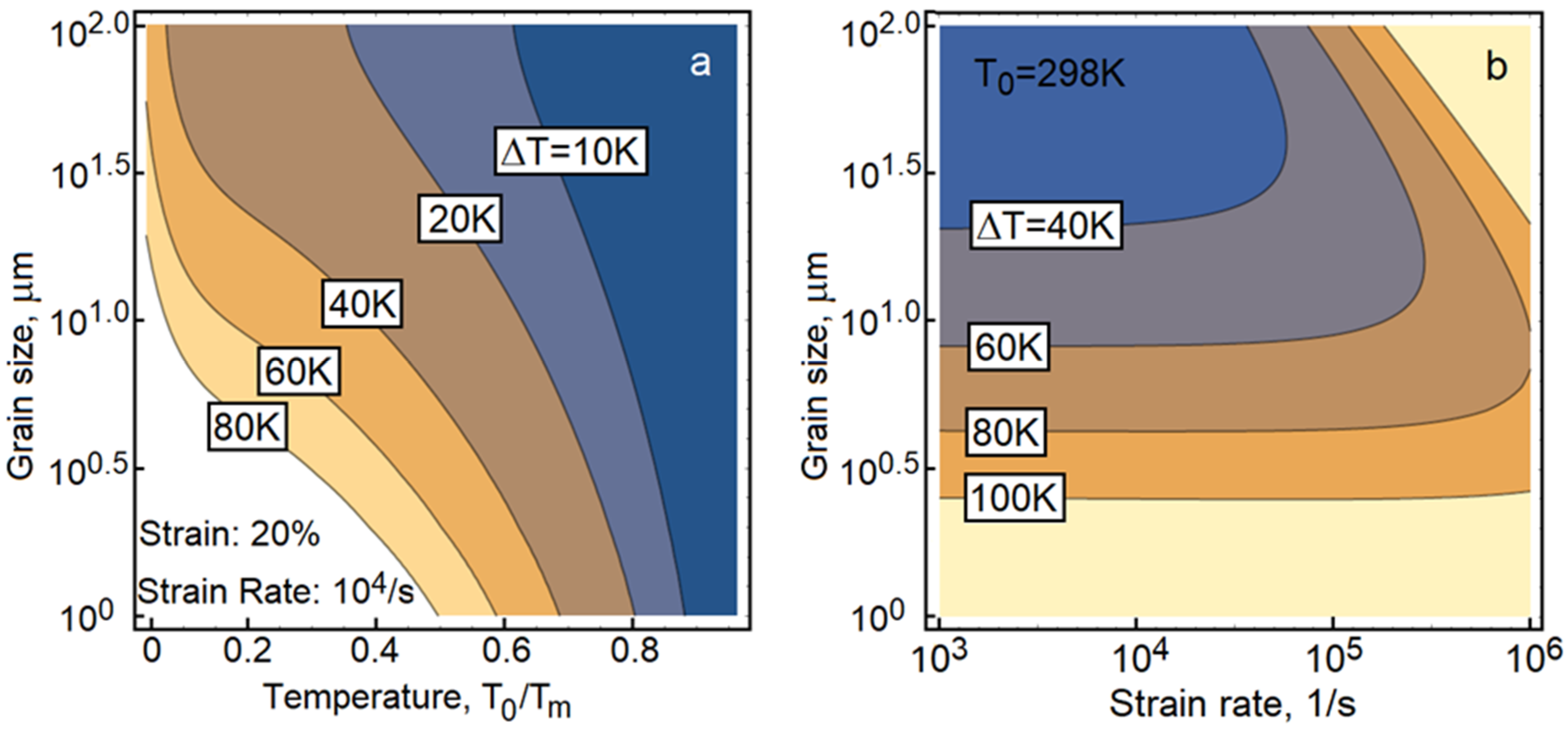
The relation is further simplified, where equivalent plastic strain has already been defined and is yield stress. The Taylor–Quinney coefficient becomes. The heat sources are formed discretely both in time and space, where spatial resolution of the sources is estimated to be in a sub-micrometer range. Experimental techniques are yet to be developed for the measurement of such small-scale temperature fluctuations. Large-scale atomistic simulations might provide invaluable insight into the phenomena. It should be stated that the contours in Figure 4a,b are constructed under the assumption that the copper specimen is subjected to uniaxial compression and the temperature rise is depicted at strain 20%. The coefficient is calibrated using experimental data presented in [46]. In Figure 4a, the temperature rise is calculated as a function of grain size and initial temperature . The samples are deformed at a strain rate of. The contours indicate that plasticity-induced heating is significantly stronger in microcrystalline copper. The environment affects the rate of heating. In large-grain copper, high strain rates noticeably magnify plasticity-induced heating, while small grains make the strain rate sensitivity an irrelevant factor (see Equation (13) and Figure 4b). For example, at a strain rate of the same temperature rise is predicted in copper with average grains 2.5 μm and 77 μm. It would be very interesting and, perhaps, technologically important to experimentally validate the theoretical predictions. The grain size dependence is discussed in the next section.
7. Hall–Petch Relation
In early 1950s, Hall [10] and Petch [11] introduced a relation, which correlates yield stress with an average size of grains
In this construction, is the size-independent strength, is a constant and is the average size of grains. In this notation, yield stress corresponds to equivalent stress. The relation is generally applicable to metals and other polycrystalline materials. A few years later, Armstrong [12] proposed a dislocation pileup interpretation and further explained the mechanism in numerous writing [47]. In this construction, the parameter is considered a Griffith type stress intensity factor, where the grain size strengthening results from the dislocation pileup along slip bands blocked at a grain boundary, thus behaving similarly to a shear crack. Among other descriptions, it is worth mentioning the concept by Ashby [48]. In Ashby’s formula, the constant includes the additional term. It will be shown that the term is reproduced in the proposed energy-based formula. Strong experimental evidence exists that dislocation pileups are responsible for the observed heterogeneous distribution of stresses. The supporting evidence was obtained in micro-diffraction (DAXM) experiments further supported by high-resolution electron backscatter diffraction (HR-EBSD) measurements [49]. It is worth noting that nanoindentation tests [50] have shown that the material hardness increases in the proximity of grain boundaries. Thus, the experimental results convey a clear message that dislocation pileups near grain boundaries are indeed responsible for the stress and energy heterogeneities.
The Hall–Petch interpretation is based on the postulate that, at a given rate of plastic strain, the upsurge of plastic power is controlled by the increases of yield stress . Here, the constraints magnify the effective yield stress. When assuming that the Hall–Petch relation prevails, one can obtain. Next, I construct a kinematics-based interpretation. At the prescribed stress, the resistance is responsible for slowing down the plastic flow. For this reason, we write . The two interpretations represent the upper and lower bound estimates of the size effect.
7.1. Energy-Based Hall–Petch Relation
I propose an energy-based interpretation of the Hall–Petch strengthening. As stated above, the Hall–Petch size effect is mostly caused by grain boundaries, which slow down the plastic flow. Suppose that polycrystalline metal is subjected to stress. This stress activates slip inside grains, but the deformation is blocked at grain boundaries. Grain boundaries are energy barriers defined in terms of surface energy. At stress, the barriers are partly climbed. As loading advances, blocked dislocations magnify the pileup stress. It should be stated that dislocations are emitted in other areas, such as grain boundary corners. After some time (the delay time), the pileups accumulate sufficient energy for a dislocation to cross the barriers. In essence, it is a stochastic process. Stress concentrations appear in different locations and grow at different rates. Large grains contain a large reservoir of energy which, in turn, feeds the energy concentrations more efficiently. The pileup-stimulated increase of internal energy is taken per unit grain boundary area and becomes. The average shear stress continues to rise and becomes the macroscopic yield stress. At this point, dislocations cross the boundaries in large numbers. The average rate of energy accumulation slows down. The correction function captures the slowing down effect. When energy overcomes the energy barrier, the macroscopic plastic flow is initiated
Grain boundary area per unit volume characterizes granular structure of the polycrystal. This ratio is sensitive to the grain size, shape and number of grains in a sample. The Hall–Petch relation becomes
In this expression, the Hall–Petch mechanism is controlled by grain boundary area per unit volume. The parameter is closely related to constant in Equation (10), such that. It has been shown [51] that the grain boundary energy is linearly dependent on shear modulus multiplied by a length parameter, where the parameter specifies the grain boundary type. Thus, the relation suggests that and carries information on the metal crystallographic structure. It turns out that the parameter is a material constant in fcc and bcc metals. Based on the data collected in [52], the mean value of for fcc metals is. In bcc metals, the values are found to be. Estimates are also made for hcp metals, but the data scatter is much larger. The hcp deformation twins might be responsible for the scatter. As usual, the magnitude of the Burgers vector is denoted by.
In Equation (12), the grain boundary area per unit volume is the size variable. The variable can be estimated with the use of stereology methods [53]. In bulk samples composed of nearly equiaxed grains, the average size of grains is about. However, the validity of the approximation can be questioned in samples with a small number of grains. The grain shape matters too. In one case, yield stress is significantly reduced in thin films of nickel, where the film’s thickness is comparable with the size of grains [54]. In the case of mild steel, Armstrong [12] made similar observations.
7.2. Kinematics-Based Construction of Hall–Petch Relation
At constant stress, energy barriers slow down plastic flow and, in this manner, affect plastic power . In the energy-based construction, the term in becomes . The pre-existing resistance to plastic flow becomes a quantifiable material constant
Now, it becomes clear that the resistance to plastic flow is strongly dependent on the size of grains. In microcrystalline copper, the value of is approaching one, thus the size effect becomes less pronounced. As shown in Section 5, the resistance is a function of relaxation time. The length is directly related to the grain boundary area per unit volume and is. Based on the above, the relaxation time becomes the size-dependent material property
It is worth stating that relaxation time (Equation (14)) matches earlier estimates made for OFHC copper [55,56]. In nanocrystalline copper, relaxation time is in the range of hundred picoseconds. The kinematically-based Hall–Petch relation fits well the existing experimental data in [52] (Figure 5). Similar trends are reported for other metals [52,57] as well.
8. Transitional Viscoplasticity
Plastic power is expressed in terms of equivalent stress and strain rate . During active deformation processes, plastic power aids to configurational entropy (suppleness [25]) of the material. The rate of true plastic strain is defined in terms of the effective rate , where the resistance-free strain rate is a function of equivalent stress and the relation is
The power-law viscoplasticity was first introduced in [58,59]. Strength is determined at 0.2% strain, where is athermal strength. Exponent determines the elastic-plastic transition. What makes the relation uncommon is that the strain rate sensitivity is further tuned by the rate factor, where and are constants and. The normalized rate of total strain completes the expression. As shown earlier, the average Schmid factor reflects slip plane misorientations, where the exponent controls the evolution of the process (Figure 1). Advances of plastic deformation broaden the spectrum of active planes and, therefore,.
At the initial stage of deformation, the rate of elastic strain dominates and, therefore, we have. At advanced deformation, plastic flow takes over and the mechanism evolves, accordingly. Thus, there is a smooth transition from diffusional flow to dislocation glide, where we should note that.
9. OFHC Copper
The constitutive model captures copper responses in a broad range of temperature and strain rates, predicts ductile damage, accounts for the size of grains, and includes the description of plasticity-induced heating. There are three groups of parameters. Parameters readily available in the literature are listed in Table 1. Among the constants are elastic properties, mass density, yield stress at 0.2% strain, Burgers vector, melting point and specific heat.
Several parameters display a marginal variability. Among the parameters are the quasi-static strain-rate sensitivity, stress exponent, thermal efficiency of plastic flow, crystallographic constant, the initial distribution of slip planes, the transition temperature and the rate of defect formation. The parameters are shown in Table 2. In the absence of experimental data, the constants should properly approximate responses of fcc metals.
The material-specific parameters are listed in Table 3. Among them are the activation energy constants , the strength pre-factor , critical energy, hardening strain and damage parameters. In this group, the activation energy constants show low variability and, therefore, there are only five fully tunable constants. One may argue that the total number of parameters is large. It is worth noting that the parameters have well-defined interpretations and most of them are material constants. I emphasize that the constitutive model captures material responses in a very broad range of temperature and strain rates, predicts ductile damage, accounts for the size of grains, and includes plasticity-induced heating.
The model capabilities are summarized in the deformation map (Figure 6), where stress at 20% strain is plotted as a function of strain rate and temperature. Two maps are constructed. In Figure 6a, the average grain size is 80 μm.
The red points depict experimental data collected from several sources [5,35,36,37,38,39,40,41,42,43,60,61,62] and the blue mesh represents the model predictions. The model correctly predicts copper responses (grains 80 μm) at temperatures from cryogenic environments up to melting points and strain rates from quasi-static loading to extreme strain rates. The second plot in Figure 6b is constructed for microcrystalline copper, where the grain size is 1 μm. Note that in the second case the stress upturn is nearly gone. This result matches experimental measurements performed on small-grained tantalum [14] and copper [15]. The strain rate sensitivity was also studied in nickel [63], where ultrafine-grained nickel exhibits a diminishing rate-sensitivity.
For completeness, I included selected stress–strain responses (Figure 7). The predictions (solid lines) are calculated at three temperatures and three strain rates. The experimental data points (red, blue and black dots) are collected from [37,61]. In all cases, I included the contribution of plasticity-induced heating, where specific heat varies with temperature.
10. Plate Impact Problem
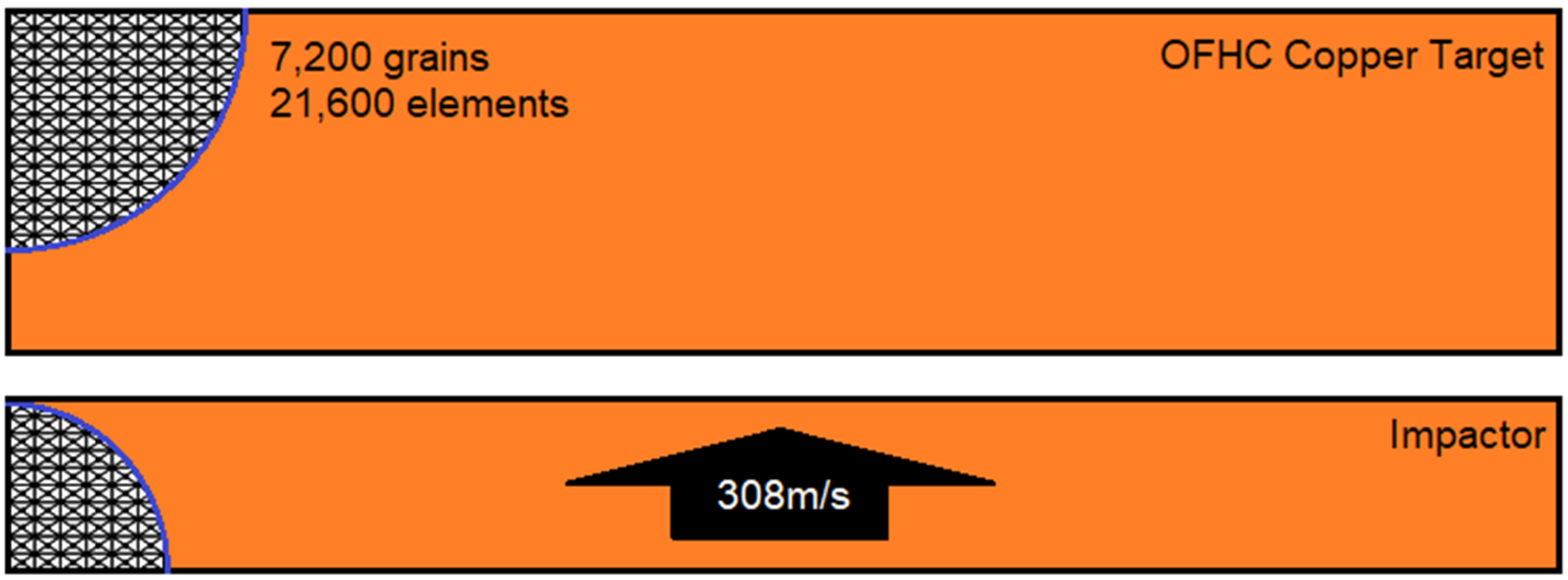
The constitutive model is implemented to a code of deformable discrete element method (DDEM). In DDEM, each discrete element represents a crystallographic grain. The grains experience large deformation and are subjected to translation and rotation, where the rigid motions are directly measurable quantities. A more detailed description of the method is presented in Appendix A. In the DDEM construction shown in Figure 8, the Cu flyer is discretized with the use of 7200 elements, while the Cu target is composed of 14,400 elements. The thicknesses of the flyer and target are 1.9 mm and 3.9 mm, respectively. The flyer travels with velocity 308 m/s and, after striking the target, shock waves are sent into both of the samples.
A simple Mie Gruneisen equation of state for copper is used. The equation is further modified to account for the contribution of dynamic excitations. It is worth stating that the calculations are made without the use of artificial viscosity. In Figure 9, VISAR measurements [64] are compared with the results of this simulation. Note that the constitutive model correctly predicts the entire impact responses, and this includes the pull-back signals. Four points, A, B, C and D, are selected for plotting contours of damage. The damage is scaled between zero and one, as described in Section 5. The scaling factor refers to the degradation of elastic properties from zero (no damage) to one (open crack). The damage factor is determined in terms of plasticity-induced dilatation. As discussed earlier, the volume change is triggered by slip incompatibilities in tension. The contact between flyer and target experiences periodic separations. The spallation damage is clearly seen in the middle section of the target. Less severe damage is noticed in other areas of the samples. The damages might be responsible for the observed ringing in the VISAR plot.
11. Conclusions
The paper summarized a five-year effort aimed for the development of a mechanisms-based viscoplasticity concept for metals. The constitutive description comprises of several novel ideas.
- The macroscopic plastic flow results from plastic slippages and slip reorganizations. The description is constructed on the basis of the tensor representation concept. It is my conviction that tensor representations derived for generic dyads represent useful tools in the hands of a modeler.
- In the proposed model, thermally activated processes are considered stochastic. The concept explains the transition of flow mechanisms from power-law creep to high strain rate dislocation glide.
- The proposed description of plasticity-induced heating is based on the hypothesis that plasticity-induced heating quantifies the efficiency of the plastic flow process, while plastic work aids in configurational entropy (suppleness) of the material.
- Drag on dislocations is activated by dynamic excitations. As shown, the excitations result from the kinematically-necessary readjustments of flow pathways.
- The stress–strain relations are constructed in the framework of transitional viscoplasticity. The power-law relations enable a smooth elastic-plastic transition during loading and unloading processes.
- I developed an energy-based Hall–Petch relation, where the commonly known stress-based relation is replaced by its kinematics-based counterpart. The proposed Hall–Petch concept was born out of extensive discussions with Ron Armstrong, who walked me through the sixty years of Hall–Petch interpretations, for which I am grateful.
- The model is calibrated for OFHC copper, implemented to a deformable discrete element code (my Ph.D. thesis) and validated in simulations of a plate impact problem. The method itself describes a semi-Cosserat medium, where grain translations and rotations are accounted for.
The most important conclusion of the study is that the flow mechanisms, transitional viscoplasticity, thermal activation, drag on dislocations and size effect are inseparable parts of the constitutive description.
Funding
This research received no external funding.
Acknowledgments
The work was supported by Alek and Research Associates, LLC. I wish to acknowledge Prof. Ron Armstrong for sharing his inside into the six decades of the Hall–Petch relation. It was a unique learning experience, for which I am grateful. I am thankful to Prof. Mick Brown for explaining his prospective on the role of self-organized criticality in plastic flow. I would like to thank Prof. Dany Rittel for offering constructive comments and suggestions.
Conflicts of Interest
The author declare no conflict of interest.
Appendix A. A Short Note on Deformable Discrete Element Method
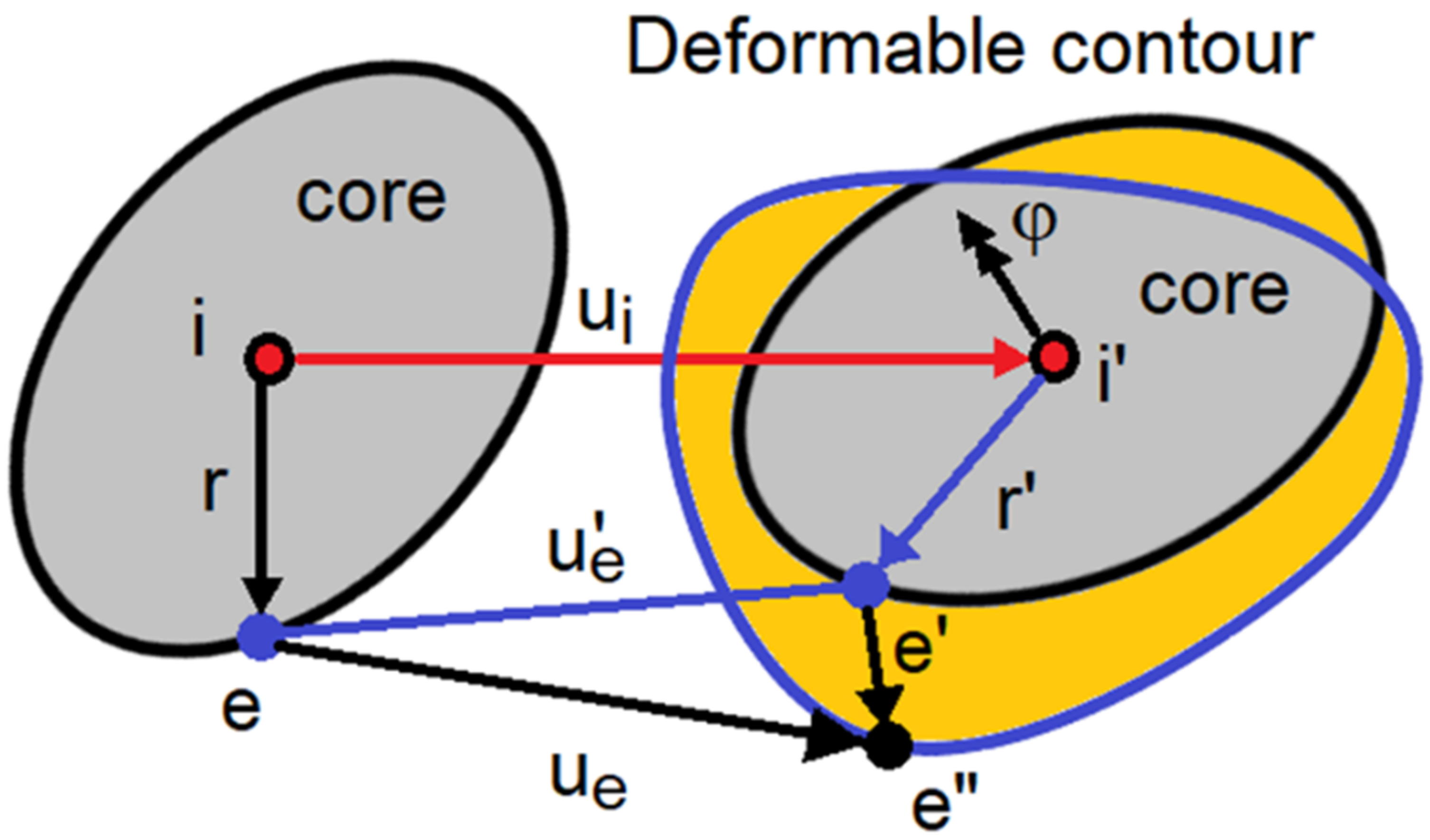
The deformable discrete element method (DDEM) was first reported in [65]. I believe that this might be one of the first if not the first DEM approach used for the prediction of fracture processes in otherwise continuum media. A complete description of the method can be found in [66]. Later, the method was reduced to a system of rigid blocks and springs, while the description of deformable particles was forgotten. Here, I describe the method as originally developed. Each particle is subjected to translations and rotations (Figure A1). In addition, each particle experiences deformation as defined in the classic finite element method. In a general case, particle rotations act on moments and, in this way, the system represents a pseudo-Cosserat medium. In this approach, mass and moments of inertia are placed in the particle mass centers. Some portion of mass is also lumped into external nodes of each particle. As a result, equations of motion are constructed in internal and external nodes.
Figure A1.
Motion and deformation of discrete element.

The motion of deformable particles includes translations and rotations of mass centers (i-nodes), while particle-to-particle interactions are defined in e-external nodes. The particle deformation is measured in terms of relative displacements between points and. The relations become. In this expression, vectors connect selected external node with the mass center. The deformation matrix links strains and relative displacements
The rotational deformation is defined with respect to the mass center and is
where. The relative displacements represent rotational deformation subtracted from the rigid core rotations. Each internal node is coupled with external nodes. The rotation-induced strain is responsible for additional storage of elastic energy , where the parameter scales the rotational constraints. Nodal forces in each element are collected from all sub-elements and are
Stress is calculated in deformable particles and is. Lastly, equations of motion are constructed in external nodes and mass centers (internal nodes)
During an active deformation process, particles may become separated, and then, the number of interconnected nodes may vary. Forces in mass centers are collected from external nodes. Moments are calculated as described in Equation (A4). In this notation, mass in external nodes is denoted , mass and moment of inertia in internal nodes are and. In DDEM, mass is redistributed between external and internal nodes in such a manner that inertia forces due to rotations and translations are decoupled. Finite elements (particles) can be subjected to large reshaping and repositioning. Thus, the DDEM method is not just a numerical solver, but it carries information on the size and potential shape of grains.
References
- Meyers, M.S.; Jarmakani, H.; Bringa, E.M.; Remington, B.A. Dislocations in shock compression and release. In Dislocations in Solids; Hirth, J.P., Kubin, L., Eds.; North-Holland: Amsterdam, The Netherland, 2009; Volume 15, pp. 91–197. [Google Scholar]
- Follansbee, P.S. High-strain-rate deformation of FCC metals and alloys. In Proceedings of the EXPLOMET ’85—International Conference on Metallurgical Applications of Shock Wave and High Strain-Rate Phenomena, Portland, OR, USA, 28 July 1985. [Google Scholar]
- Kumar, A.; Kumble, R.G. Viscous drag on dislocations at high strain rates in copper. J. Appl. Phys. 1969, 40, 3475–3480. [Google Scholar] [CrossRef]
- Regazzoni, G.; Kocks, U.F.; Follansbee, P.S. Dislocation kinetics at high strain rates. Acta Metall. 1987, 35, 2865–2875. [Google Scholar] [CrossRef]
- Bragov, A.; Igumnov, L.; Konstantinov, A.; Lomunov, A.; Rusin, E. Effects of high strain rate on plastic deformation of metal materials under fast compression loading. J. Dyn. Behav. Mater. 2019, 5, 309–319. [Google Scholar] [CrossRef]
- Dodd, B.; Bai, Y. Adiabatic Shear Localization: Frontiers and Advances, 2nd ed.; Elsevier: Amsterdam, The Netherlands, 2012; pp. 2–18. [Google Scholar]
- Bever, M.B.; Holt, D.L.; Titchener, A.L. The stored energy of cold work. Prog. Mater Sci. 1973, 17, 5–177. [Google Scholar] [CrossRef]
- Farren, W.S.; Taylor, G.I. The heat developed during plastic extension of metals. Proc. R. Soc. A 1952, 5, 398–451. [Google Scholar]
- Taylor, G.I.; Quinney, H. The latent energy remaining in a metal after cold working. Proc. R. Soc. A 1934, 143, 307–326. [Google Scholar]
- Hall, E.O. The deformation and aging of mild steel. Proc. Phys. Soc. Lond. 1951, 64, 747–753. [Google Scholar] [CrossRef]
- Petch, N.J. The cleavage strength of polycrystals. J. Iron Steel Inst. 1953, 174, 25–28. [Google Scholar]
- Armstrong, R.W. On size effect in polycrystal plasticity. J. Mech. Phys. Solids 1961, 9, 196–199. [Google Scholar] [CrossRef]
- Armstrong, R.W.; Codd, L.; Douthwaite, R.M.; Petch, N.J. The plastic deformation of polycrystalline aggregates. Philos. Mag. 1962, 7, 45–58. [Google Scholar] [CrossRef]
- Park, H.-S.; Rudd, R.E.; Cavallo, R.M.; Barton, N.R.; Arsenlis, A.; Belof, J.L.; Blobaum, K.J.M.; El-Dasher, B.S.; Florando, J.N.; Huntington, C.M.; et al. Grain-size-independent plastic flow at ultrahigh pressures and strain rates. Phys. Rev. Lett. 2015, 114, 065502. [Google Scholar] [CrossRef]
- Mao, Z.N.; An, X.H.; Liao, X.Z.; Wang, J.T. Opposite grain size dependence of strain rate sensitivity of copper at low vs high strain rates. Mater. Sci. Eng. A 2018, 738, 430–438. [Google Scholar] [CrossRef]
- Arzt, E. Size effects in materials due to microstructural and dimensional constraints: A comparative review. Acta Mater. 1998, 46, 5611–5626. [Google Scholar] [CrossRef] [Green Version]
- Pande, C.S.; Cooper, K.P. Nanomechanics of Hall-Petch relationship in nanocrystalline materials. Prog. Mater. Sci. 2009, 54, 689–706. [Google Scholar] [CrossRef]
- Zerilli, F.J.; Armstrong, R.W. Dislocation-mechanics-based constitutive relations for material dynamics calculations. J. Appl. Phys. 1987, 61, 1816–1825. [Google Scholar] [CrossRef] [Green Version]
- Johnson, G.R.; Cook, W.H. A constitutive model and data for metals subjected to large strains, high strain rates and high. In Proceedings of the 7th International Symposium, Ballistics, The Hague, 19–21 April 1983; pp. 541–547. [Google Scholar]
- Follansbee, P.S.; Kocks, U.F. A constitutive description of the deformation of copper based on the use of the mechanical threshold. Acta Metall. 1988, 36, 81–93. [Google Scholar] [CrossRef] [Green Version]
- Preston, D.L.; Tonks, D.L.; Wallace, D.C. Model of plastic deformation for extreme loading conditions. J. Appl. Phys. 2003, 93, 211–220. [Google Scholar] [CrossRef] [Green Version]
- Salvado, F.C.; Teixeira-Dias, F.; Walley, S.M.; Lea, L.J.; Cardoso, J.B. A review on the strain rate dependency of the dynamic viscoplastic response of fcc metals. Prog. Mater. Sci. 2017, 88, 186–231. [Google Scholar] [CrossRef] [Green Version]
- Gurrutxanga-Lerma, B. A stochastic study of the collective effect of random distribution of dislocations. J. Mech. Phys. Solids 2019, 124, 10–34. [Google Scholar] [CrossRef] [Green Version]
- Langer, J.S. Statistical thermodynamics of crystal plasticity. J. Stat. Phys. 2019, 175, 531–541. [Google Scholar] [CrossRef] [Green Version]
- Brown, L.M. Power laws in dislocation plasticity. Philos. Mag. 2016, 96, 2696–2713. [Google Scholar] [CrossRef]
- Richeton, T.; Weiss, J.; Louchet, F. Dislocation avalanches: Role of temperature, grain size and strain hardening. Acta Mater. 2005, 53, 4463–4471. [Google Scholar] [CrossRef]
- Zaiser, M.; Nikitas, N. Slip avalanches in crystal plasticity: Scaling of avalanche cutoff. J. Stat. Mech. Theory Exp. 2007, 2007, P04013. [Google Scholar] [CrossRef]
- Pantheon, W. Distribution in dislocation structures: Formation and spatial correlation. J. Mater. Res. 2002, 17, 2433–2441. [Google Scholar] [CrossRef]
- Zubelewicz, A. Micromechanical study of ductile polycrystalline materials. J. Mech. Phys. Solids 1993, 41, 1711–1722. [Google Scholar] [CrossRef]
- Zubelewicz, A. Tensor Representations in Application to Mechanisms-Based Constitutive Modeling; Technical Report ARA-2; Alek & Research Associates, LLC: Los Alamos, NM, USA, 2015. [Google Scholar] [CrossRef]
- Zubelewicz, A. Overall stress and strain rates for crystalline and frictional materials. Int. J. Non Linear Mech. 1991, 25, 389–393. [Google Scholar] [CrossRef]
- Zubelewicz, A. Metal behavior at extreme loading rates. Mech. Mat. 2009, 41, 969–974. [Google Scholar] [CrossRef]
- Armstrong, R.W.; Walley, S.M. High strain rate properties of metals and alloys. Int. Mater. Rev. 2008, 53, 105–128. [Google Scholar] [CrossRef]
- Ryu, S.; Kang, K.; Cai, W. Entropic effect on the rate of dislocation nucleation. Proc. Natl. Acad. Sci. USA 2011, 108, 5174–5178. [Google Scholar] [CrossRef] [Green Version]
- Kubin, L.P. Dislocation patterns: Experiment, theory and simulations. In Stability of Materials; Plenum Press: New York, NY, USA, 1996; pp. 99–135. [Google Scholar]
- Gray, G.T.; Chen, S.R.; Wright, W.; Lopez, M.F. Constitutive Equations for Annealed Metals under Compression at High Strain Rates and High Temperature; IS-4 Report, LA-12669-MS; Los Alamos National Laboratory: Los Alamos, NM, USA, 1994.
- Gray, G.T., III. High strain rate deformation: Mechanical behavior and deformation substructures induced. Annu. Rev. Mater. Res. 2012, 42, 285–303. [Google Scholar] [CrossRef]
- Gao, C.Y.; Zhang, L.C. Constitutive modelling of plasticity of fcc metals under extremely high strain rates. Int. J. Plast. 2012, 32–33, 121–133. [Google Scholar] [CrossRef]
- Huang, S.H.; Clifton, R.J. Macro and Micro-Mechanics of High Velocity Deformation and Fracture; Kawata, K., Shioiki, J., Eds.; IUTAM: Tokyo, Japan, 1985; pp. 63–74. [Google Scholar]
- Tong, W.; Clifton, R.J.; Huang, S.H. Pressure-shear impact investigation of strain rate history effects in oxygen-free high-conductivity copper. J. Mech. Phys. Solids 1992, 40, 1251–1294. [Google Scholar] [CrossRef]
- Nemat-Nasser, S.; Li, Y. Flow stress of fcc polycrystals with application to OFHC Cu. Acta Mater. 1988, 46, 565–577. [Google Scholar] [CrossRef]
- Tanner, A.B.; McGinty, R.D.; McDowell, D.L. Modeling temperature and strain rate history effects in OFHC Cu. Int. J. Plast. 1999, 15, 575–603. [Google Scholar] [CrossRef]
- Baig, M.; Khan, A.S.; Choi, S.-H.; Jeong, A. Shear and multiaxial responses of oxygen free high conductivity (OFHC) copper over wide range of strain-rates and temperatures and constitutive modeling. Int. J. Plast. 2013, 40, 65–80. [Google Scholar] [CrossRef]
- Jordan, L.J.; Siviour, C.R.; Sunny, G.; Bramlette, C.; Spowart, J.E. Strain rate-dependent mechanical properties of OFHC copper. J. Mater. Sci. 2013, 48, 7134–7141. [Google Scholar] [CrossRef]
- Rittel, D.; Zhang, L.H.; Osovski, S. The dependence of the Taylor-Quinney coefficient on the dynamic loading mode. J. Mech. Phys. Solids 2017, 107, 96–114. [Google Scholar] [CrossRef]
- Nieto-Fuentes, J.C.; Rittel, D.; Osovski, S. On a dislocation-based constitutive model and dynamic thermomechanical considerations. Int. J. Plast. 2018, 108, 55–69. [Google Scholar] [CrossRef]
- Armstrong, R.W. Size effect on material yield strength/deformation/fracturing properties. J. Mater. Res. 2019, 34. [Google Scholar] [CrossRef]
- Ashby, M.F. The deformation of plasticity non-homogeneous materials. Philos. Mag. 1970, 21, 399–424. [Google Scholar] [CrossRef]
- Guo, Y.; Collins, D.M.; Tarleton, E.; Hofmann, F.; Tischler, J.; Liu, W.; Xu, R.; Wilkinson, A.J.; Britton, T.B. Measurements of stress fields near a grain boundary: Exploring blocked arrays of dislocations in 3D. Acta Mater. 2015, 96, 229–236. [Google Scholar] [CrossRef] [Green Version]
- Voyiadjis, G.Z.; Zhang, C. The mechanical behavior during nanoindentation near the grain boundary in a bicrystal fcc metal. Mater. Sci. Eng. A 2015, 621, 218–228. [Google Scholar] [CrossRef]
- Udler, D.; Seidman, D.N. Grain boundary and surface energies of fcc metals. Phys. Rev. B 1996, 54, 133–136. [Google Scholar] [CrossRef] [Green Version]
- Cordero, Z.C.; Knight, B.E.; Schuh, C.A. Six decades of the Hall-Petch effect—A survey of grain-size strengthening studies on pure metals. Int. Mater. Rev. 2016, 61, 495–512. [Google Scholar] [CrossRef]
- Van Vlack, L.H. Elements of Materials Science and Engineering, 6th ed.; Addison Wesley: Boston, MA, USA, 1989. [Google Scholar]
- Keller, C.; Hug, E.; Retoux, R.; Feaugas, X. TEM study of dislocation patterns in near-surface and core regions of deformed nickel polycrystals with few grains across the cross section. Mech. Mater. 2010, 42, 44–54. [Google Scholar] [CrossRef]
- Zubelewicz, A. Metal behavior in the extremes of dynamics. Sci. Rep. 2018, 8, 5162. [Google Scholar] [CrossRef] [Green Version]
- Zubelewicz, A. Century-long Taylor-Quinney interpretation of plasticity-induced heating reexamined. Sci. Rep. 2019, 9, 9088. [Google Scholar] [CrossRef] [Green Version]
- Ravi Chandran, K.S. A new exponential function to represent the effect of grain size on the strength of pure iron over multiple length scales. J. Mater. Res. 2019, 34, 2315–2324. [Google Scholar] [CrossRef]
- Zubelewicz, A.; Addessio, F.L.; Cady, C. Constitutive model for uranium-niobium alloy. J. Appl. Phys. 2006, 100, 013523. [Google Scholar] [CrossRef]
- Zubelewicz, A.; Zurek, A.K.; Potocki, M.L. Dynamic behavior of copper under extreme loading rates. J. Phys. IV 2006, 134, 23–27. [Google Scholar] [CrossRef]
- Chen, S.R.; Kocks, U.F. On the strain rate dependence of dynamic recrystallization in copper polycrystals. In Proceedings of the International Conference Recrystallization 92, San Sebastian, Spain, 31 August–4 September 1992. [Google Scholar]
- Freed, A.D.; Walker, K.P. High temperature constitutive modeling: Theory and applications. In Proceedings of the Winter Annual Meeting of the American Society of Mechanical Engineers, Atlanta, GA, USA, 1–6 December 1991. [Google Scholar]
- Banerjee, B. An evaluation of plastic flow stress models for the simulation of high-temperature and high-strain-rate deformation of metals. arXiv 2005, arXiv:cond-mat/0512466. [Google Scholar] [CrossRef]
- Selyutina, N.S.; Borodin, E.N.; Petrov, Y.V. Structural-temporal peculiarities of dynamic deformation of nanostructured and nanoscaled metals. Phys. Solid State 2018, 60, 1813–1820. [Google Scholar] [CrossRef]
- Thomas, S.A.; Veeser, L.R.; Turley, W.D.; Hixson, R.S. Comparison of CTH simulations with measured wave profiles for simple flyer plate experiments. J. Dyn. Behav. Mater. 2016, 2, 365–371. [Google Scholar] [CrossRef] [Green Version]
- Zubelewicz, A. Iterative method of finite elements. In Proceedings of the 2nd Conference on Computational Methods in Mechanics of Structures, Gdansk, Poland, 24–26 November 1975. [Google Scholar]
- Zubelewicz, A. A Certain Version of Finite Element Method. Ph.D. Thesis, Warsaw University of Technology, Warsaw, Poland, 1979. [Google Scholar]
Figure 1.
Slip-events distribution around the dominant plane θ = 0.

Figure 2.
Path rerouting activates dynamic excitations. Note that overstress is only partly stored in newly created dislocation structures.
Figure 2.
Path rerouting activates dynamic excitations. Note that overstress is only partly stored in newly created dislocation structures.

Figure 3.
Stress at strain 20% is plotted as a function of strain rate. The data points are collected from [3,36,37,38,39,40,41,42,43,44].

Figure 4.
Contours of temperature rise are plotted as a function of grain size. (a) Temperature rise is calculated at strain rate 104/s and in a broad range of initial temperatures T0. (b) Temperature rise is plotted at room temperature and for strain rates between 103/s and 106/s. The coefficient is estimated based on experimental measurements in [46].

Figure 5.
Grain size strengthening depicted at strains approximately one percent. Experimental data (blue points) gathered from [52]. The red line represents the model predictions. The middle part of the log–log plot complies with the Hall–Petch relation.
Figure 5.
Grain size strengthening depicted at strains approximately one percent. Experimental data (blue points) gathered from [52]. The red line represents the model predictions. The middle part of the log–log plot complies with the Hall–Petch relation.

Figure 6.
Deformation maps for copper presented in terms of stress at 20% strain. The blue mesh represents the model predictions taken in a broad range of temperatures and strain rates. (a) Experimental data collected from References [5,35,36,37,38,39,40,41,42,43,60,61,62] and the points are marked in red. (b) Microcrystalline copper (grains size 1 μm) does not exhibit the stress upturn.

Figure 7.
Selected stress–strain responses are constructed for three strain rates and three temperatures. The average size of grains is assumed to be 80 μm. The data is collected from [37,61].

Figure 8.
Copper target is struck by a copper flyer with velocity 308 m/s. The entire system is constructed with the use of 7200 triangle particles, where each particle is composed of three elements. Artificial viscosity is not used in this simulation.
Figure 8.
Copper target is struck by a copper flyer with velocity 308 m/s. The entire system is constructed with the use of 7200 triangle particles, where each particle is composed of three elements. Artificial viscosity is not used in this simulation.

Figure 9.
VISAR measurement (thick gray line) reported in [64] is compared with results of the numerical simulation (red line). Damage levels from zero (no damage) to one (fully developed crack) are shown at VISAR points A, B, C and D. The contours are rescaled to fit the window.
Figure 9.
VISAR measurement (thick gray line) reported in [64] is compared with results of the numerical simulation (red line). Damage levels from zero (no damage) to one (fully developed crack) are shown at VISAR points A, B, C and D. The contours are rescaled to fit the window.


Table 1.
Text-book material constants.
| Bulk Modulus | Shear Modulus | Mass Density | Yield Stress, 298 K | Burgers Vector | Melting Point | Specific Heat, 298 K |
|---|---|---|---|---|---|---|
| 385 |
Table 2.
Material constants with marginal variability.
| Strain Rate Exponent | Stress Exponent | Heat Coefficient | Crystallographic Constant | Schmid Factor | Transition Temperature | Overstress Exponent |
|---|---|---|---|---|---|---|
| 0.5 |
Table 3.
Material-specific parameters.
| Activation Energy Factor | Thermal Activation | Stress Pre-Factor | Critical Energy | Schmid Factor | Ductility | Damage Strain |
|---|---|---|---|---|---|---|
© 2020 by the author. Licensee MDPI, Basel, Switzerland. This article is an open access article distributed under the terms and conditions of the Creative Commons Attribution (CC BY) license (http://creativecommons.org/licenses/by/4.0/).
Share and Cite
MDPI and ACS Style
Zubelewicz, A. Mechanisms-Based Transitional Viscoplasticity. Crystals 2020, 10, 212. https://doi.org/10.3390/cryst10030212
AMA Style
Zubelewicz A. Mechanisms-Based Transitional Viscoplasticity. Crystals. 2020; 10(3):212. https://doi.org/10.3390/cryst10030212
Chicago/Turabian StyleZubelewicz, Aleksander. 2020. "Mechanisms-Based Transitional Viscoplasticity" Crystals 10, no. 3: 212. https://doi.org/10.3390/cryst10030212
Note that from the first issue of 2016, this journal uses article numbers instead of page numbers. See further details here.