
Equilibrium Selection in Hawk–Dove Games
1
Department of Business and Management Science, Norwegian School of Economics, 5045 Bergen, Norway
2
Research Institute of Industrial Economics, SE-102 15 Stockholm, Sweden
*
Author to whom correspondence should be addressed.
Games 2024, 15(1), 2; https://doi.org/10.3390/g15010002
Submission received: 25 November 2023
/
Revised: 21 December 2023
/
Accepted: 27 December 2023
/
Published: 31 December 2023
(This article belongs to the Special Issue Applications of Game Theory to Industrial Organization)
Abstract
:We apply three equilibrium selection techniques to study which equilibrium is selected in a hawk–dove game with a multiplicity of equilibria. By using a uniform-price auction as an illustrative example, we find that when the demand in the auction is low or intermediate, the tracing procedure method of Harsanyi and Selten (1988) and the quantal response method of McKelvey and Palfrey (1998) select the same equilibrium. When the demand is high, the tracing procedure method does not select any equilibrium, but the quantal response method still selects the same equilibrium as when the demand is low or intermediate. The robustness to strategic uncertainty method of Andersson, Argenton and Weibull (2014) selects two of the multiple equilibria irrespective of the demand size. We also analyze the impact of an increase in the minimum bid allowed by the auctioneer in the equilibrium selection.
Keywords:
hawk–dove games; equilibrium selection; tracing procedure method; robustness to strategic uncertainty method; quantal response methodJEL Classification:
C72; C79; D44; D471. Introduction
The hawk–dove game is one of the salient models used to study a wide range of questions in the industrial organization literature. In the classical representation of the game, players compete by using two strategies—hawk and dove. In this case, the hawk–dove game has two possible Nash equilibria in pure strategies—one of the players behaves as a hawk and the other as a dove. As both players prefer the equilibrium in which they select the hawk strategy and the opposing player selects the dove strategy, which equilibrium emerges between two individuals in any given iteration of the game is ambiguous—either of the two pure-strategy Nash equilibria could be played. To break the ambiguity associated with a multiplicity of equilibria, numerous equilibrium selection methods have been proposed.
We analyze in detail the outcome of three different equilibrium selection methods applied to a hawk–dove game in which we extend the set of strategies and consequently, the set of possible Nash equilibria. The extension of the set of strategies helps us to capture many real-world situations where the players can choose among a large strategy set. In each of those equilibria, as in the basic two-strategy hawk–dove game, one of the players behaves as a dove, the other as a hawk, and both prefer the equilibrium in which the other player selects the dove strategy. We apply the tracing procedure method of Harsanyi and Selten (1988) [1], the robustness to strategic uncertainty method of Andersson, Argenton and Weibull (2014) [2], and the quantal response method of McKelvey and Palfrey (1998) [3] to predict which equilibrium is selected by the players.
We frame the hawk–dove game as a uniform-price auction1 in which two players with asymmetric production capacities2 compete to satisfy an inelastic demand.3 Having observed the demand, the players simultaneously and independently submit a bid for their entire production capacity, assumed to be lower than the total demand. That is, each player faces a positive residual demand when it is dispatched last in the auction. The auctioneer establishes the maximum and the minimum bids that can be submitted in the auction. The player that submits the higher bid sets the price and satisfies the residual demand, while the player that submits the lower bid is dispatched first and satisfies the total demand at the price set by the other player. In the case of a tie, the players are dispatched in proportion to their production capacity4.
The game described above has multiple pure-strategy Nash equilibria in which one of the players submits the maximum bid allowed by the auctioneer (dove strategy) and the opponent submits a bid that makes undercutting unprofitable (hawk strategy). As in the classic representation of the hawk–dove game, the players have opposing preferences for both sets of equilibria; each player prefers the set of equilibria in which the opposing player submits the maximum bid allowed by the auctioneer (dove strategy), since in that case the player dispatched first sells its entire production capacity at the maximum price allowed by the auctioneer.
When the demand is low or intermediate in the auction, the tracing procedure method of [1] and the quantal response method of [3] select the same equilibrium. When the demand is instead high, the tracing procedure method does not select any equilibrium, but the quantal response method still selects the same equilibrium as when the demand is low or intermediate. An increase in the minimum bid allowed by the auctioneer does not change the equilibrium selected, but it does worsen the coordination in the selected equilibrium when the tracing procedure is applied and makes coordination easier when the quantal response method is applied. The robustness to strategic uncertainty method proposed by [2] selects two of the multiple equilibria irrespective of the demand size and the minimum bid allowed by the auctioneer.
In a similar setup, Boom 2008 Ref. [8] applies the tracing procedure method to predict the equilibrium selected by the players in a uniform-price auction. The author also assumes uniform prior beliefs, but restricts the set of strategies that can be selected by the players to the strategies that are part of a Nash equilibria. By restricting the set of strategies, the author finds that with independence of the demand realization, the tracing procedure always selects the equilibrium in which the player with the higher production capacity submits the maximum bid (dove strategy), since the players always deviate to a pair of strategies that is a Nash equilibrium. In contrast, we do not restrict the set of strategies5 and we find that the tracing procedure only selects the equilibrium in which the player with the higher production capacity submits the maximum bid (dove strategy) when the demand is low or intermediate, but when the demand is high, no equilibrium is selected by the tracing procedure. This is because the players deviate to a pair of strategies that are not a Nash equilibrium, and a miscoordination problem emerges.
Our paper is related to the industrial organization literature, which endogenizes the emergence of a price leader in duopoly models, in two respects. First, we endogenize the emergence of a price leader, in our case, in a uniform-price auction. Second, due to the multiplicity of equilibria, we also apply the tracing procedure to study which equilibrium is selected in the game. In particular, Ref. [9] focus on a model with homogeneous products, linear demand, constant marginal cost, and with one firm being more efficient than the other. Using an endogenous timing game introduced by Hamilton and Slutksky (1990) [10], the authors apply the tracing procedure method to show that the player with the lower production costs emerges as a leader in a Stackelberg model with a continuous set of strategies. Ref. [11] focus on a model with price competition in a duopoly with differentiated substitutable products, linear and symmetric demand, and constant marginal cost. In contrast to the models of quantity competition, when the players compete in prices, the leadership role is not the most preferred one. This result is in line with other models of price competition with capacity constraints [12,13,14].
The emergence of a price leader when applying the tracing procedure has also been studied in experimental settings. In particular, Ref. [15] use a vertical product differentiation model with two asymmetric players, first choosing qualities and then choosing prices, in order to design an experiment with the structure of a Battle of the Sexes game. The tracing procedure method applied to their theoretical framework and their experimental results predict that the higher the degree of asymmetry of the game, the higher the predictive power of the tracing procedure method. These results are in line with our results, but in contrast to the experimental design proposed by [15], where the players compete only by setting two prices, we provide a theoretical framework where the players compete using more than two strategies.
The hawk–dove game can also be analyzed using other approaches. Using behavioural economics, Ref. [4] study coordination failures in a context of inequality. They study this relationship by running an experiment where the authors vary the degree of inequality and efficiency of an allocation problem. They frame the experiment as a hawk–dove game that illustrates a typical trade-off where two agents compete for the appropriation of a scarce resource, and each can choose whether to fight or accommodate. The authors find that an increase in inequality facilitates the coordination in one of the equilibria.6 We complement their analysis using a game theoretical approach, where we apply the tracing procedure, the robustness to strategic uncertainty method, and the quantal response methods to a hawk–dove game. Following the quantum game theory approach applied to the 2008 financial crisis, Ref. [16] finds that hawks “exhibit low entanglement with others and thus behave classically, whereas Doves exhibit higher, leading to more quantum behavior”. The analysis suggests that hawks could be induced to reduce risky, destructive trading practices by raising their entanglement.
The article proceeds as follows. Section 2 describes the set-up, the timing, and the equilibrium of the game. Section 3, Section 4 and Section 5 apply the tracing procedure method, the robustness to strategic uncertainty method, and the quantal response method, respectively, to the game and study the equilibrium selected by the players. Section 6 concludes the paper. The proofs are in Appendix A. In Appendix B, we provide an example to illustrate the theoretical analysis. In Appendix B, we also describe the algorithms that we apply in the computational simulations used in the paper. In Appendix C, we provide a complete discussion of the tie-breaking rule and its importance in the paper.
2. Model
In this section, we present the set-up and the timing of a uniform-price auction, and we characterize the equilibrium.
Set-up: There are two players, h and l, with production capacity and , respectively, where . The level of demand, , is perfectly inelastic. Moreover, , i.e., the demand is large enough to guarantee that both players face a positive residual demand. We introduce this assumption because when the demand is very low , both players have enough production capacity to satisfy the demand individually. In that case, the resulting Nash equilibrium is unique, and selection methods are no longer useful.
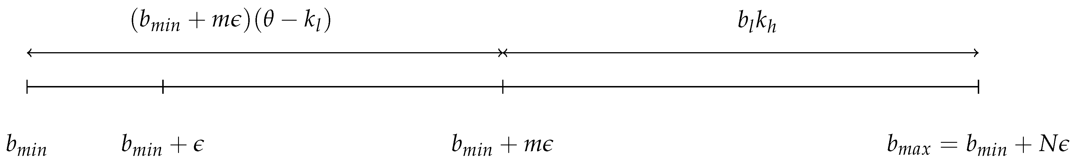
Timing: Having observed the realization of demand , each player simultaneously and independently submits a bid specifying the lowest price at which it is willing to supply up to its capacity, , , where and are determined by the auctioneer. The players can only submit bids higher than or equal to and lower than or equal to .7 The number of bids in that interval (N) is determined exogenously and it can be freely set. The minimum bid increment between one bid and the next is defined by . Let m be an integer between 1 and N. The set of strategies is represented in Figure 1.
Let denote a bid profile. On the basis of this profile, the auctioneer calls players into operation. The output allocated to player h (player l’s output is symmetric), denoted by , is given by:8
When player h submits the lower bid, it sells its entire production capacity . When both players submit the same bid, the demand is split among them in proportion to their production capacity . When player h submits the higher bid, it satisfies the residual demand .
Finally, the payments are worked out by the auctioneer. When the auctioneer runs a uniform-price auction, the price received by a player for any positive quantity dispatched by the auctioneer is equal to the higher offer price accepted in the auction. Hence, player h’s payoffs9 (in the paper, we write all the equations from the viewpoint of player h; the equations for player l follow the same structure), denoted by , are given by:10
When player h submits the lower bid, it sells its entire production capacity , and player l sets the price . Therefore, player h’s payoffs are . When players h and l submit the same bid, the payoff is split among them in proportion to their production capacity .11 When player h submits the higher bid, it satisfies the residual demand , and it sets the price . Therefore, player h’s payoffs are .
Equilibrium: The uniform-price auction described above has a multiplicity of pure-strategy equilibria defined by:
In each of the equilibria defined in Equation (3), one player submits the maximum bid (dove strategy), and the other submits a bid that makes undercutting unprofitable (hawk strategy). When the players are asymmetric in production capacity, the set of equilibria in which the player with the higher production capacity submits the maximum bid is larger than the set of equilibria in which the player with the lower production capacity submits the maximum bid. To provide a better understanding of the uniform-price auction and the set of equilibria in that game, in Appendix B (Figure A4), we provide an illustrative example. That is the example that we use in all the numerical simulations in the paper.
The players have opposite preferences on both sets of equilibria. Both players prefer the set of equilibria in which the opposing player submits the maximum bid (dove strategy), since in that case the player that is dispatched first sells its entire production capacity at the highest possible price.
3. Tracing Procedure Method
In this section, we study which equilibrium is selected by the tracing procedure method when we apply it to the uniform-price auction presented in the model section [1]. We also study the impact of an increase in the minimum bid allowed by the auctioneer on the selected equilibrium.
The tracing procedure method assumes that players’ payoffs12 are a linear combination of the original payoff matrix and the expected payoff matrix based on players’ beliefs:
In Equation (4), represents the original payoff matrix for player h (Equation (2)), and represents the expected payoff matrix based on player h’s beliefs. In , is the probability that player l assigns to each strategy based on player h’s beliefs.13 Therefore, when , players’ payoffs are determined only by players’ expected payoff based on their prior beliefs. When , players’ payoffs are determined only by the original payoff matrix.
In general, at the players choose a pair of strategies that is not an equilibrium of the original game. When t increases, the players change their strategies. At some , the players chose a pair of strategies that is an equilibrium of the original game [1]. That pair of strategies ) will be the equilibrium selected by the tracing procedure method. Therefore, the key point in the tracing procedure method is to find the player that first deviates to a Nash equilibrium in the original game, and to find the parameter t for which the deviation occurs.
In Lemma 1, we analyse player h’s expected payoff when that player has uniform prior beliefs about player l’s strategies.
Lemma 1.
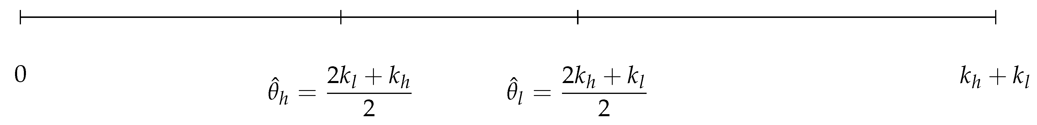
When all players have uniform prior beliefs about the strategies played by other players, and when the demand is low , both players maximize their expected payoff by submitting the minimum bid. When the demand is intermediate , player h maximizes its expected payoff by submitting the maximum bid allowed by the auctioneer and player l maximizes its expected payoff by submitting the minimum bid allowed by the auctioneer. When the demand is high , both players maximize their expected payoff by submitting the maximum bid.
Lemma 1 determines the low, intermediate, and high demand thresholds (Equations (A3)–(A5), Appendix A, and Figure 2). When the demand is low , both players maximize their expected payoff by submitting the minimum bid allowed by the auctioneer (left-hand panel, Figure 3). When the demand is intermediate , player h maximizes its expected payoff by submitting the maximum bid allowed by the auctioneer and player l maximizes its expcted payoff by submitting the minimum bid allowed by the auctioneer (central panel, Figure 3). When the demand is high , both players maximize their expected payoff by submitting the maximum bid allowed by the auctioneer (right-hand panel, Figure 3). These two thresholds determine the demand for which the players prefer to submit the minimum or the maximum bid at the beginning of the tracing procedure method . This result is formalized in Proposition 1.
Proposition 1.
When , the tracing procedure method selects one of the three possible types of equilibria.
- i.
- Low demand : Both players submit a bid equal to the minimum bid allowed by the auctioneer.
- ii.
- Intermediate demand : The player with the higher production capacity submits the maximum bid, and the player with the lower production capacity submits the minimum bid allowed by the auctioneer.
- iii.
- High demand : Both players submit a bid equal to the maximum bid.
When , the players’ total payoffs are determined only by the expected payoffs. When the demand is low , the players’ residual demand is very low, and it is very risky for them to submit a high bid. Therefore, both players maximize their expected payoffs by submitting the minimum bid allowed by the auctioneer (left-hand panel, Figure 3). In this case, the equilibrium selected by the tracing procedure method when is . When the demand is intermediate , the player with the higher production capacity faces a high residual demand and maximizes its expected payoff by submitting the maximum bid. In contrast, the player with the lower production capacity faces a low residual demand and maximizes its expected payoff by submitting the minimum bid allowed by the auctioneer (central panel, Figure 3). In that case, the equilibrium selected by the tracing procedure method when is (). Finally, when the demand is high , both players face a high residual demand and they maximize their expected payoff by submitting the maximum bid allowed by the auctioneer (right-hand panel, Figure 3). In that case, the equilibrium selected by the tracing procedure method when is .
It is easy to check that when and the demand is intermediate, the tracing procedure method immediately selects one of the Nash equilibria in the original game. Therefore, it is not necessary to conduct further analysis. In contrast, when and the demand is low or high, the players do not select one of the Nash equilibria in the initial game, and it is necessary to determine which player deviates first to a Nash equilibrium in the original game and to find the parameter t for which that player deviates to the equilibrium. Proposition 2 formalizes this analysis.
Proposition 2.
When the demand is low or intermediate , the tracing procedure method selects the equilibrium in which the player with the higher production capacity submits the maximum bid, and the player with the lower production capacity submits the minimum bid allowed by the auctioneer. When the demand is high , no equilibrium is selected by the tracing procedure method.
According to Proposition 1, when and the demand is low, both players submit the minimum bid allowed by the auctioneer (left-hand panel, Figure 3). When , the players assign more weight to the original payoff matrix , and one of the players has incentives to deviate by raising its bid. Given that for the same pair of strategies , , player h deviates first. Once player h raises its bid, player l is better off for two reasons: first, because it maximizes its expected payoffs , and second, because it sells its entire production capacity for a higher price. When t increases, player h continues raising its bid until the equilibrium is selected (left-hand panel, Figure 4).
According to Proposition 1, when and when the demand is intermediate, the tracing procedure method selects the equilibrium , i.e., it selects an equilibrium in the original game (central panel, Figure 3). Therefore, is the equilibrium selected by the tracing procedure, since the players do not deviate when t increases.
According to Proposition 1, when and the demand is high, both players submit the maximum bid allowed by the auctioneer (right-hand panel, Figure 3). When , the players assign more weight to the original payoff matrix , and one of the players has incentives to deviate by decreasing its bid, since by doing so it will be dispatched first, selling its entire production capacity at the maximum bid allowed by the auctioneer. In contrast to the case when the demand is low, the player that does not deviate is worse off, since it will serve the residual demand. Therefore, it has incentives to undercut the other player, initiating a price war. It is important to note that the price war does not select any equilibrium, since at some , one of the players has incentives to submit the maximum bid allowed by the auctioneer generating cycles and not selecting any equilibrium. This contrasts with [8], where the players always deviate to one equilibrium, since in that paper, the set of strategies is restricted to the strategies that belong to the equilibrium.
We conclude this section by studying the impact that an increase in the minimum bid allowed by the auctioneer has on the equilibrium selected by the tracing procedure method.
Proposition 3.
When the demand is low ,14 an increase in the minimum bid allowed by the auctioneer has two effects on the convergence to the equilibrium.
- i.
- The parameter t for which the players deviate from the equilibrium when increases.
- ii.
- The parameter t for which the players coordinate in one of the Nash equilibria of the original game increases.
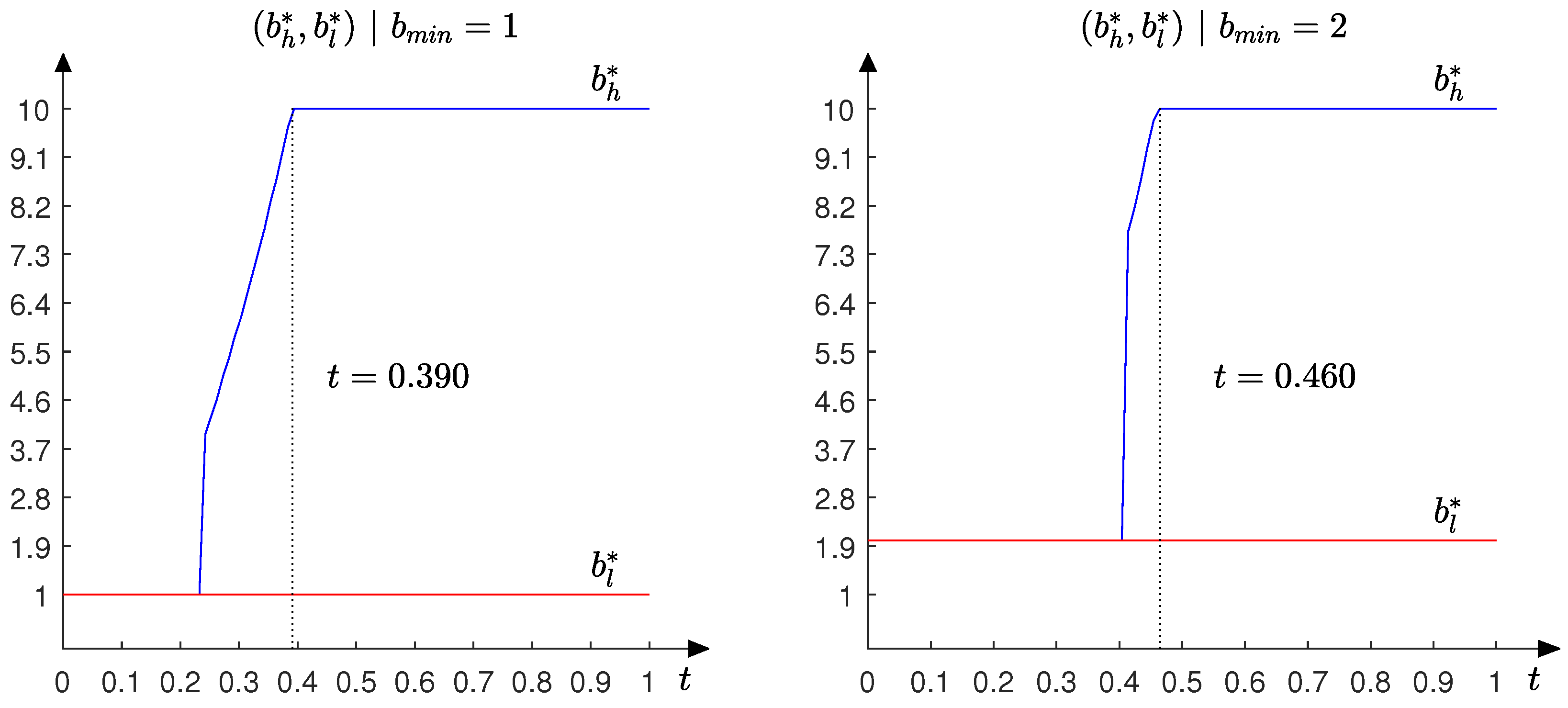
An increase in the minimum bid allowed by the auctioneer makes submitting a low bid more attractive, since in this case, both players split the demand in proportion to their production capacity at a higher price. Therefore, the parameter t that makes them deviate from the equilibrium in the tracing procedure method when increases. As can be observed in the left-hand side of Figure 4, when the minimum bid allowed by the auctioneer is low, the parameter t for which the players coordinate in one of the equilibria of the game is . However, as can be observed in the right-hand panel of that figure, when the minimum bid allowed by the auctioneer increases to , the corresponding value of t is .
In the numerical simulations, we have also observed that the bid that makes players indifferent between submitting the minimum bid and deviating to a higher bid also increases. Therefore, when the players deviate from the original equilibrium in the tracing procedure method, they deviate by submitting a higher bid. As can be observed in the left-hand panel in Figure 4, when the minimum bid allowed by the auctioneer is low , the player with the higher production capacity deviates first by increasing its bid to . However, as can be observed in the right-hand panel of that figure, when the minimum bid allowed by the auctioneer increases to , the player with the higher production capacity deviates by increasing its bid to .
The theoretical results in Proposition 3 have important welfare implications, since an increase in the minimum bid makes coordinating in one of the equilibria of the game more difficult for the players. Therefore, the expected equilibrium price can be lower, since the players do not coordinate in one of the equilibria in which the equilibrium price is equal to the maximum bid.
4. Robustness to Strategic Uncertainty Method
In this section, we study which equilibrium is selected by the robustness to strategic uncertainty method when we apply it to the uniform-price auction presented in the model section [2]. We also study the impact of an increase in the minimum bid allowed by the auctioneer in the selected equilibrium.
The robustness to strategic uncertainty method proposes that players face some uncertainty about the strategies played by other players. Player h’s uncertainty about player l’s strategy is modeled as follows:
where the random variables are statistically independent.
Equation (5) can be interpreted as follows: player h thinks that player l will play strategy plus some random perturbation. When the uncertainty parameter (t-parameter) goes to zero, the players do not face any uncertainty.
For , the random variable has a probability density defined by:
A pair of strategies is a t-equilibrium of the game if and maximize (6). Therefore, to find the t-equilibrium of the game, it is enough to work out the best response functions and to find the intersection between them.
If we apply Equation (6) to the payoff function in the uniform-price auction model defined by Equation (2), we obtain:
where is the cumulative distribution function of . The first term in Equation (7), , represents player h’s expected payoff when it submits the lower bid in the auction. With probability , player h submits the lower bid in the auction. In that case, player l sets the price (), and player h sells its entire production capacity (). The second term in Equation (7), , represents player h’s expected payoff when it submits the higher bid in the auction. With probability , player h submits the higher bid in the auction. In that case, player h sets the price () and satisfies the residual demand .
Using Equation (7), it is easy to work out one player’s expected payoff given the strategy of the other player. In particular, we set and vary between and . Knowing that the random variable has a probability density defined by , and if, as in [2], we assume that , we work out player h’s expected payoff , and we choose that maximizes that payoff. Repeating that process for every , we work out player h’s best response function. Using the same approach, we work out player l’s best response function. The intersection between both players’ best response functions determines the equilibrium selected by the robustness to strategic uncertainty method.
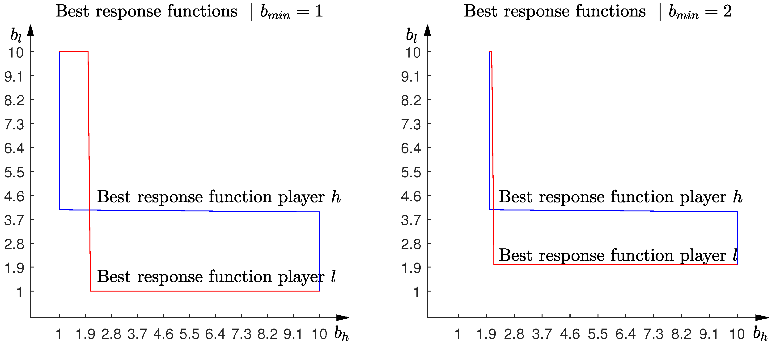
In Figure 5, we plot the players’ best response functions. When one player submits a low bid, the best strategy for the other player is to submit a high bid. The players shift from low to high bids when the opponent player submits a bid around the threshold that determines the set of Nash equilibria (Equation (3)). The intersection of the best response functions selects two of the Nash equilibria in the original game. In each of these two equilibria, one player submits the maximum bid and the other player submits the minimum bid allowed by the auctioneer.
We conclude this section studying the impact that an increase in the minimum bid allowed by the auctioneer has on the equilibrium selected by the robustness to strategic uncertainty method. An increase in the minimum bid allowed by the auctioneer reduces the set of Nash equilibria (right-hand panel, Figure 5). However, the equilibrium selected by the robustness to strategic uncertainty method does not change. As in the case when the minimum bid allowed by the auctioneer is lower, the robustness to strategic uncertainty method selects the equilibria in which one player submits the minimum bid and the other player submits the maximum bid (right-hand panel, Figure 5).
5. Quantal Response Method
In this section, we study which equilibrium is selected by the quantal response method when we apply it to the uniform-price auction presented in the model section [3]. We also study the impact of an increase in the minimum bid allowed by the auctioneer in the selected equilibrium.
The quantal response method assumes that the players choose among the strategies in the game based on their relative expected payoff. The key idea is that when the players calculate their expected payoff, they make calculation errors according to some random process. Based on that random process, the players assign more probability to the strategies that give a higher expected payoff. The Nash equilibrium in the quantal response method is the set of probabilities for which none of the players wants to deviate. Formally, the Nash equilibrium in the quantal response method is defined as follows: Given , a sequence such that , and , a corresponding sequence with for all t such that , then is a Nash equilibrium.
In their seminal paper, [3] use the logistic quantal response function. That specific function is a particular parametric class of quantal response functions that has a long tradition in the study of individual choice behaviour. The logit equilibrium correspondence is the correspondence given by:
where the term in the numerator is one of the players’ expected payoff when it selects strategy i and the other player selects strategy j.16 The term in the denominator is the sum of one of the players’ expected payoff when it selects strategy i and the other player selects all the strategies in its set of strategies. Therefore, by using Equation (8), each player assigns more probability to the strategies that give it a higher expected payoff.
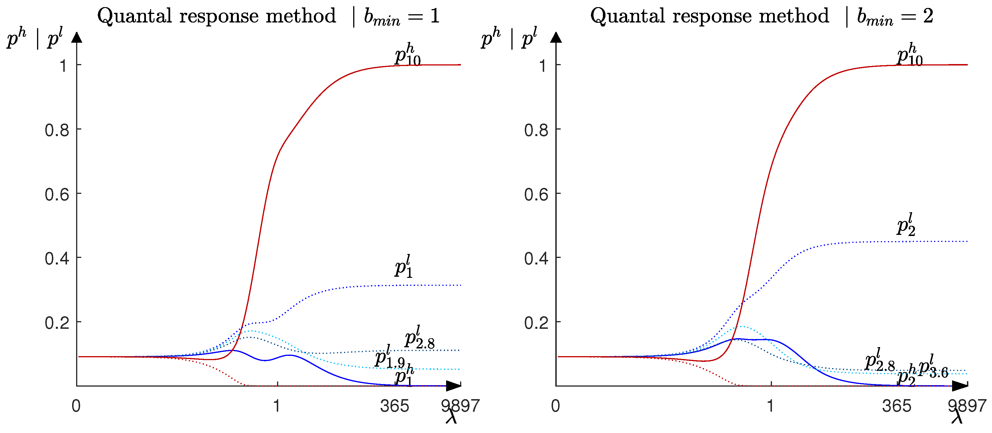
When we apply the quantal response method to the uniform-price auction presented in the model section, we observe that the player with the higher production capacity (player h) plays the maximum bid with a probability close to one (continuous red line ) and the minimum bid with a probability close to zero (continuous blue line ). In contrast, the player with the lower production capacity (player l) assigns higher probabilities to the lower bids (discontinuous blue line , , ) (left-hand panel, Figure 6)17.
The equilibrium selected by the quantal response method is in line with the equilibrium selected by the tracing and the robustness to strategic uncertainty methods. Moreover, the pattern that appears in the equilibrium selected by the quantal response method is very similar to the pattern that appears in the other two methods, since in the three methods the players tend to select extreme strategies. In particular, the player with the higher production capacity submits the maximum bid and the player with the lower production capacity submits the lower bids in the strategies supported with higher probabilities. Moreover, the quantal response method shows similarities to the tracing procedure method, since the quantal response method defines a unique selection from the set of Nash equilibria by “tracing” the graph of the logit equilibrium correspondence beginning at the centroid of the strategy simplex (the unique solution when ) and continuing for larger and larger values of .
We conclude this section by analyzing the effect that an increase in the minimum bid allowed by the auctioneer has on the equilibrium selected by the quantal response method. After an increase in the minimum bid allowed by the auctioneer, player h assigns probability one to the maximum bid allowed by the auctioneer and player l assigns higher probabilities to the lower bids in the strategies’ support (left-hand panel, Figure 6). An increase in the minimum bid does not change the strategy of the player with the higher production capacity, since it still faces a high residual demand and does not change its strategy (continuous red line ), but makes it more attractive for the player with the lower production capacity to submit lower bids, since for that player, the expected payoff associated with low bids increases (discontinuous blue lines , , ).18 Therefore, an increase in the minimum bid allowed in the auction facilitates the coordination in the equilibrium of the game where the player with the higher production capacity submits the maximum bid allowed by the auctioneer. This contrasts with the results that we obtain when we apply the tracing procedure method, where an increase in the minimum bid allowed by the auctioneer reduces the possibilities that the players coordinate in that equilibrium.
6. Conclusions
Hawk–dove games are widely used in the industrial organization literature. Such games have a multiplicity of Nash equilibria. In each of those equilibria, one of the players submits the maximum bid (dove strategy) and the other player submits a bid that makes undercutting unprofitable (hawk strategy). By framing the hawk–dove game as a uniform-price auction, we apply the tracing procedure method [1], the robustness to strategic uncertainty method [2], and the quantal response method [3] to predict which equilibrium is selected by the players. We also analyze the impact of an increase in the minimum bid allowed by the auctioneer on the equilibrium selection.
The equilibrium selected by the tracing procedure method proposed by [1] depends crucially on the realization of the demand. When the demand is low or intermediate, the tracing procedure method selects the equilibrium in which the player with the higher production capacity submits the maximum bid (dove strategy) and the player with the lower production capacity submits the minimum bid allowed by the auctioneer (hawk strategy). When the demand is high, the tracing procedure method does not select any equilibrium. This contrasts with [8], where the tracing procedure method always selects the equilibrium in which the player with the higher production capacity submits the maximum bid (dove strategy). When the auctioneer increases the minimum bid allowed in the auction, the equilibrium selected by the players does not change, but the coordination in that equilibrium is more difficult.
The robustness to strategic uncertainty method proposed by [2] selects the two equilibria in which one of the players submits the maximum bid (dove strategy) and the other player submits the minimum bid allowed by the auctioneer (hawk strategy). When the auctioneer increases the lower bid allowed in the auction, the equilibria selected by the players do not change.
The quantal response method proposed by [3] predicts that the player with the higher production capacity submits the maximum bid (dove strategy) with probability one and the player with the lower production capacity submits the lower bids in the strategy set with higher probabilities (hawk strategy). An increase in the minimum bid allowed by the auctioneer does not change the strategy of the player with the higher production capacity, but increases the probability that the low-production-capacity player assigns to the minimum bid, and the coordination in one of the equilibria of the game is easier.
The theoretical results that we present in this paper contribute to the industrial organization literature that endogenize the emergence of a price leader in duopoly models. We also extend the literature of hawk–dove games, since, in our paper, the players can choose among a large set strategies.
The theoretical analysis that we have developed also gives us the opportunity to compare the equilibrium played in a uniform-price auction with the one played in a discriminatory-price auction. Therefore, the theoretical framework that we develop could be useful for comparing the results among different auction types.
We have discussed that there appears to be no clear consensus in the literature on the definition and the relationship between “hawk–dove” and “Battle-of-Sexes” games. In this paper, we assume that a game has the structure of a “hawk–dove” game when it follows the structure presented in [7], and we applied three different equilibrium selection methods to it. The analysis in our paper is useful in fostering research into the relationship between the “hawk–dove” and “Battle-of-Sexes” games and the equilibrium that emerges in these games. We leave that analysis for future research.
Author Contributions
Conceptualization, M.B.d.P. and N.K.; methodology, M.B.d.P. and N.K.; software, M.B.d.P. and N.K.; validation, M.B.d.P. and N.K.; formal analysis, M.B.d.P. and N.K.; investigation, M.B.d.P. and N.K.; writing—original draft preparation, M.B.d.P. and N.K.; writing—review and editing, M.B.d.P. and N.K.; visualization, M.B.d.P. and N.K. All authors have read and agreed to the published version of the manuscript.
Funding
This work has been funded by CINELDI—Centre for intelligent electricity distribution, an 8-year Research Centre under the FME-scheme (Centre for Environment-friendly Energy Research, 257626/E20). Mario Blázquez de Paz gratefully acknowledges financial support from the Research Council of Norway and the CINELDI partners.
Data Availability Statement
We do not use data in our paper. Therefore data sharing is not applicable.
Acknowledgments
We are very grateful to the participants at CINELDI, Norwegian University of Science and Technology, Norwegian School of Economics seminars, and EARIE and NORIO conferences.
Conflicts of Interest
The authors declare no conflicts of interest.
Appendix A
Lemma A1.
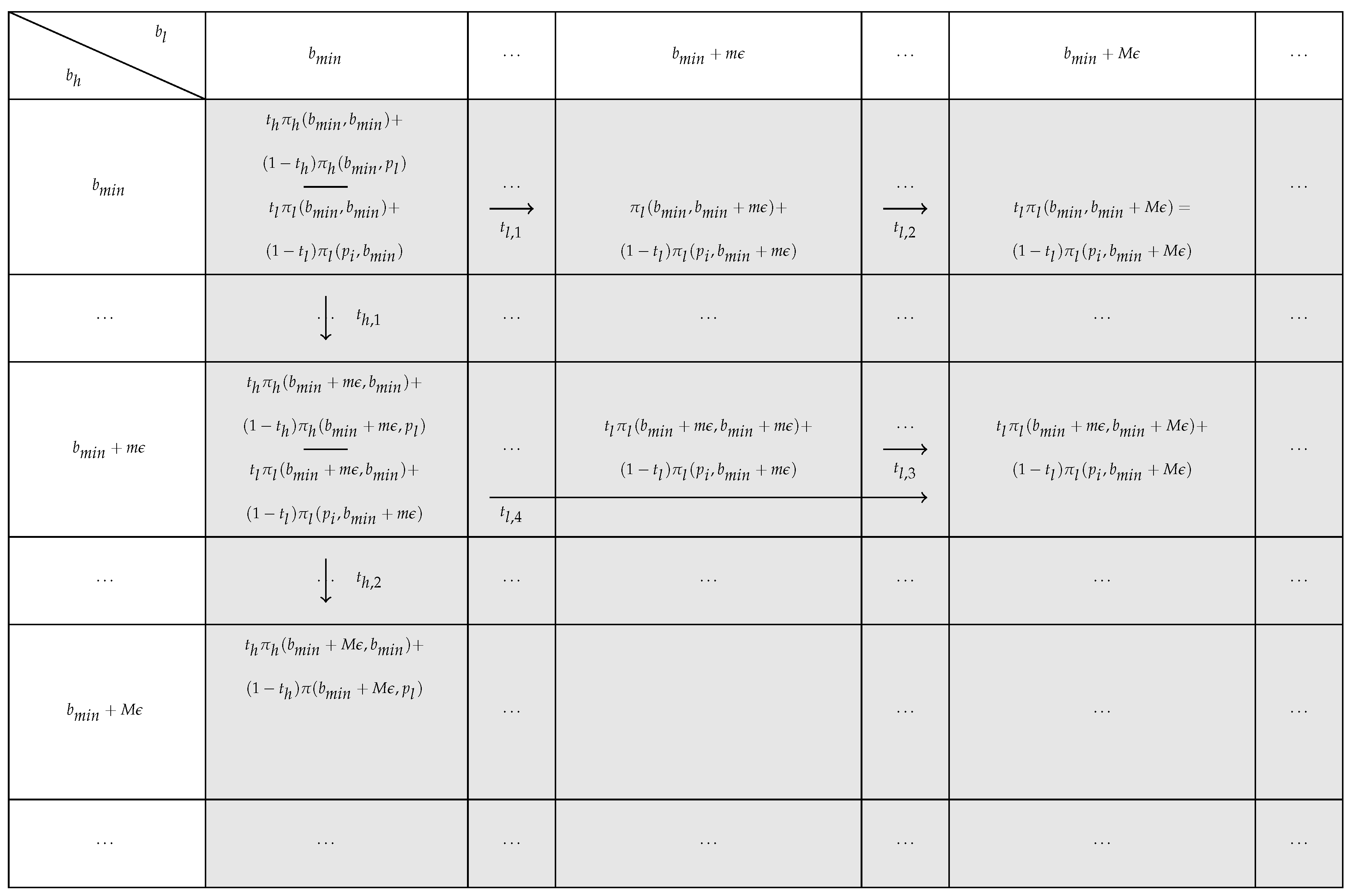
In Lemma 1, we study the relation between the structural parameters of the model (demand and production capacities) and players’ expected payoff. When player h (the proof for player l is identical) submits a bid equal to , its expected payoff is defined by , where is the minimum bid allowed by the auctioneer, m is an integer number, and is the increase between one bid and the next one and can be as small as we want by increasing N.19 N is the total number of bids in the strategy set. The set of strategies is represented in Figure A1. The probability that player l assigns to each bid in the strategy set is defined by . If the probability that each player assigns to each bid follows a uniform distribution, the closed-form solution of the expected payoff function for player h when it submits a bid is worked out as follows:
The first term in Equation (A1) represents player h’s expected payoff when it submits the higher bid in the auction. With probability , player h submits the higher bid in the auction. In that case, player h sets the equilibrium price and satisfies the residual demand . The second term in Equation (A1) represents player h’s expected payoff when player l submits the higher bid in the auction. With probability player l submits the higher bid in the auction. In that case, player l sets the equilibrium price that in expectation is equal to , and player h sells its entire production capacity .
![Games 15 00002 g0a1]()
Figure A1.
Strategy set and payoffs.

To work out the bid that maximizes the expected profit, it is necessary to work out Equation (A1)’s first-order conditions.
where the first term in Equation (A2) is positive, which means that when the player satisfies the residual demand, it increases its payoffs by increasing its bid. In contrast, the second term in Equation (A2) is negative, which means that when the player satisfies the total demand, it prefers to decrease its bid to increase its chances to be dispatched first in the auction.
After rearranging Equation (A2) to write it as a function of the structural parameters, we obtain:
The first term in Equation (A3) is always negative, and the second term is negative if . Therefore, if , is negative and player h maximizes its expected profit by submitting the lower bid in the auction. In contrast, if , player h could maximize its expected payoff at , at a critical point, or at . Therefore, it is necessary to work out the critical points and the second derivative to know which strategy maximizes the expected payoff.
To work out the critical points, it is enough to equalize Equation (A3) to zero. Therefore,
To know if the critical point is a maximum or a minimum, it is necessary to work out the second derivative.
Given that we are studying the case in which , the second term in Equation (A3) is positive, and then Equation (A5) is also positive. Therefore, the expected payoff is a concave function, and the critical point defined by Equation (A4) is a global minimum. Hence, player h maximizes its profits by submitting the lower or the higher bid allowed by the auctioneer, but not by submitting a bid equal to the critical point .
Proposition A1.
When , the players’ total payoff are determined only by the expected payoff. Therefore, the proof of Proposition A1 is straightforward using the results of Lemma A1.
Figure A2.
Proposition A2. Case i: Low demand .

Proposition A2.
Proposition A2 analyzes the equilibrium selected by the tracing procedure method when the demand is low (i), intermediate (), or high (). We analyze each case.
Case i: Low demand . We prove that when the demand is low, the tracing procedure method selects the equilibrium in which the player with the higher production capacity submits the maximum bid allowed by the auctioneer and the player with the lower production capacity submits the minimum bid allowed by the auctioneer.
In Proposition A1, we show that when , the tracing procedure method selects the equilibrium in which both players submit the minimum bid in the auction. However, that pair of strategies is not an equilibrium in the original game. Therefore, the key point in the tracing procedure method is to find the pair of strategies for each value of t until the players select a pair of strategies that are an equilibrium in the original game.
Within the proof, we use the next notation:
. solves Equation (4) for player h when it increases its bid from to while player l’s bid is (Figure A2).
. solves Equation (4) for player h when it increases its bid from to while player l’s bid is (Figure A2).
. solves Equation (4) for player l when it increases its bid from to while player h’s bid is (Figure A2).
. solves Equation (4) for player l when it increases its bid from to while player h’s bid is (Figure A2).
. solves Equation (4) for player l when it increases its bid from to while player h’s bid is (Figure A2).
. solves Equation (4) for player l when it increases its bid from to while player h’s bid is (Figure A2).
The proof consists of two steps. In step one, we prove that the player with the higher production capacity (player h) deviates first by increasing its bid from to , i.e., . In step two, we prove that once player h deviates by increasing its bid from to , it deviates first again by increasing its bid from to , i.e., . Proving step two directly is difficult, and we prove it in three different steps: . Below, we present a sketch of the four steps of the proof, and we explain the intuition behind each step.
In step one, we prove that the player with the higher production capacity (player h) deviates first from the pair of strategies by increasing its bid, i.e., we prove that , where solves and solves ( and are represented in Figure A2). Step one proves that the player with the higher production capacity adopts a “dove" strategy in the game where players’ payoff functions are defined by the tracing procedure method profits, Equation (4).
In the rest of the proof (steps two, three, and four), we need to show that once the player with the higher production capacity increases its bid, the player with the lower production capacity never deviates. The intuition is simple: in the first step, once the player with the higher production capacity increases its bid by adopting a “dove” strategy, the player that adopts a “hawk” strategy is better off and never deviates from the strategy in which it submits the minimum bid. Therefore, the player with the higher production capacity continues increasing its bid until the players select the pair of strategies . That will be the equilibrium in the original game selected by the tracing procedure method. Proving this result directly is complex, since it is necessary to show that (Figure A2). Therefore, we prove it in three different steps. In step two, we prove that . In step three, we prove that . In step four, we prove that . Putting together steps two, three, and four, we obtain .
In step two, we prove that , where solves and solves , where ( and are represented in Figure A2).
In step three, we prove that , where solves ( is represented in Figure A2).
In step four, we prove that , where solves ( is represented in Figure A2).
In the rest of the proof, we explain in detail each of the four steps. In step one, we prove that , where solves .
Therefore, is defined implicitly by:
and explicitly by the closed-form solution:
By doing some algebra in , we obtain:
Therefore,
In Equation (A7), , since the we are studying the low-demand case , and , since and . The last inequality holds to guarantee that Equation (A6) is satisfied: by Proposition A1, we know that when the demand is low, the expected payoff is decreasing, i.e., . Therefore, to guarantee that Equation (A6) is satisfied, it is necessary that . Therefore, , and that guarantees that . Moreover, , and that guarantees that .
Using Equation (A7), we can prove that . In particular, given that , it is enough to show that if , and if .
First, we prove that :
where the inequality holds since .
Second, we prove that :
where the inequality holds, since
Therefore, .
In step two, we prove , where solves .
Therefore, is defined implicitly by:
and explicitly by the closed-form solution:
By doing some algebra in and , we obtain:
In Equation (A11), , since we are studying the low-demand case and . And , since , , and . Moreover, , and that guarantees that .
Using Equation (A11), we can prove that . In particular, given that , it is enough to show that and that .
First, we prove that :
where the inequality holds, since and .
Second, we prove that :
where the inequality holds, since
Therefore, .
In step three, we prove that , where solves:
and solves:
Therefore, the closed-form solutions for and are:
Given that , if . We prove that :
where the inequality holds, since . Therefore, .
In step four, we prove that , where solves:
and solves:
Second, , and by Lemma A1, we know that . Therefore, the left-hand side in Equation (A15) is larger than the left-hand side in Equation (A14) for all . Hence, when , player l is better off by submitting than by submitting , and the parameter that makes player l deviate from to is always larger than the parameter that makes player l deviate from to , i.e., .
To summarize, when the demand is low , the player with the higher production capacity (player h) deviates first from the pair of strategies by increasing its bid (“dove” strategy), i.e., . Once that player h adopts a “dove” strategy by increasing its bid to , player l is better of by adopting a “hawk” strategy, and it never deviates from , i.e., . Therefore, player h continues increasing its bid until it submits a bid equal to the maximum bid allowed by the auctioneer. Hence, when the demand is low, the tracing procedure method selects the equilibrium in which the player with the higher production capacity submits the maximum bid and the player with the lower production capacity submits the minimum bid .
Case : Intermediate demand .
According to Lemma A1, when the demand is intermediate , the player with the higher production capacity maximizes its expected payoff by submitting the maximum bid , and the player with the lower production capacity maximizes its expected payoff by submitting the minimum bid . Therefore, when the demand is intermediate, the tracing procedure method selects the equilibrium in which the player with the higher production capacity submits the maximum bid and the player with the lower production capacity submits the minimum bid at , and the players do not deviate from that equilibrium when t increases. Therefore, when the demand is intermediate, the equilibrium selected by the tracing procedure method is .
Case : High demand .
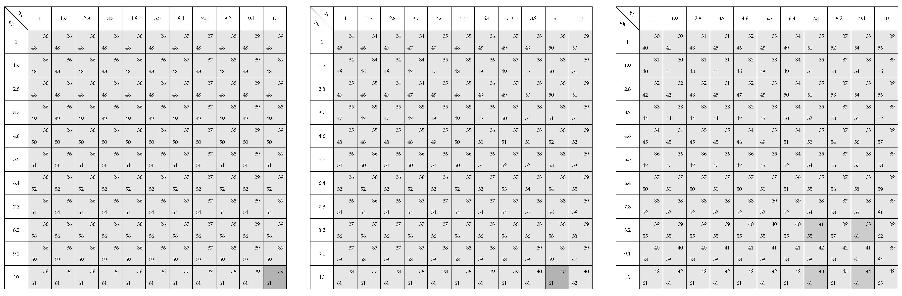
When the demand is high, the tracing procedure method does not select any of the equilibria of the original game. We illustrate this point with the example in Figure A3. As we prove in Lemma A1, when the demand is high, the players maximize their expected payoff by submitting the maximum bid (left-hand panel, Figure 3). Therefore, when , the unique Nash equilibrium is (left-hand panel, Figure A3). However, that is not an equilibrium in the original payoff matrix of the game (left-hand panel, Figure A4). Therefore, when t increases, one of the players has incentives to deviate (central panel, Figure A4). When t increases, the player with the lower production capacity deviates by undercutting the player with the higher production capacity, and the Nash equilibrium is , which is not an equilibrium in the original payoff matrix of the game. It is important to note that the player that does not deviate is worse off, since it submits the higher bid and satisfies the residual demand. Therefore, as soon as t increases a little, it decreases its bid to be dispatched first in the auction, but this triggers a price war and the other player also wants to undercut. When the bid is too low, it is not profitable any more to undercut and the player with the higher production capacity increases its bid, but in that case, the player with the lower production capacity increases its bid, but still undercutting the other player, since in that case it is dispatched first in the auction and at the same time it increases the expected payoff, since when the demand is high, the expected payoff is an increasing function. This cycle in the strategies is summarized in the right-hand panel in Figure A3.20 Therefore, when the demand is high, the tracing procedure method does not select any of the equilibria of the original game.
Figure A3.
Payoff matrix in a uniform-price auction. , , , , , .

Figure A4.
Payoff matrix in a uniform-price auction. , , , , .

Proposition A3.
i. The parameter t for which the players deviate from the equilibrium when increases.
In Equation (A7), we work out the parameter t that makes players deviate from the equilibrium when . To prove Proposition 3.i., it is enough to show that , i.e., when increases, the players stay longer at the equilibrium when .
where
In Equation (A16), the denominator is always positive. Therefore, we only need to prove that . That expression is equal to:
In Equation (A17), the term appears with positive and negative sign. Moreover, . Taking this into account, Equation (A17) can be simplified to:
where the inequality holds, since and (low demand). Therefore, , and the players stay longer at the equilibrium when . The intuition of this result is simple: when the minimum bid increases, the equilibrium is more attractive, and the players stay at that equilibrium longer.
ii. The parameter t for which the players coordinate in one of the Nash equilibria of the original game increases.
The results presented in Propositions A1 and A2 are also valid when the minimum bid allowed by the auctioneer increases . Therefore, the equilibrium selected by the players is the one in which the larger player submits the maximum bid and the player with the lower production capacity submits the minimum bid . We focus our analysis on the low-demand case, since, as we prove in Proposition A2, when the demand is intermediate, the players coordinate in the equilibrium when , and when the demand is high, the tracing procedure method does not select any equilibrium.
The value for which the players select the equilibrium when the minimum bid allowed by the auctioneer is is defined implicitly by:
and explicitly by:
The value for which the players select the equilibrium when the minimum bid allowed by the auctioneer is is defined explicitly by:
The value of has been defined in Lemma A1 as , where is the maximum bid, is the minimum bid allowed by the auctioneer, and N is the number of bids in the supported strategy. By using Lemma A1, we also define . If the difference between and is not too big, and if N is large enough, then , and Equations (A19) and (A20) can be simplified to be compared:
For further reference, we introduce:
Therefore,
Since , , and , then and . Therefore, :
The inequality in (A21) holds, since and . Therefore, .
Appendix B
In this section, we introduce an example to illustrate the theoretical results presented in the paper. We work out the tracing procedure method using the theoretical predictions in Lemma A1 and Propositions A1 and A2. We complement that analysis by using another three different methods to work out the tracing procedure method, and we show that the results are the same. We also detail the algorithm used to work out the equilibrium selected by the robustness to strategic uncertainty method. To work out the quantal response method, we apply Equation (8).
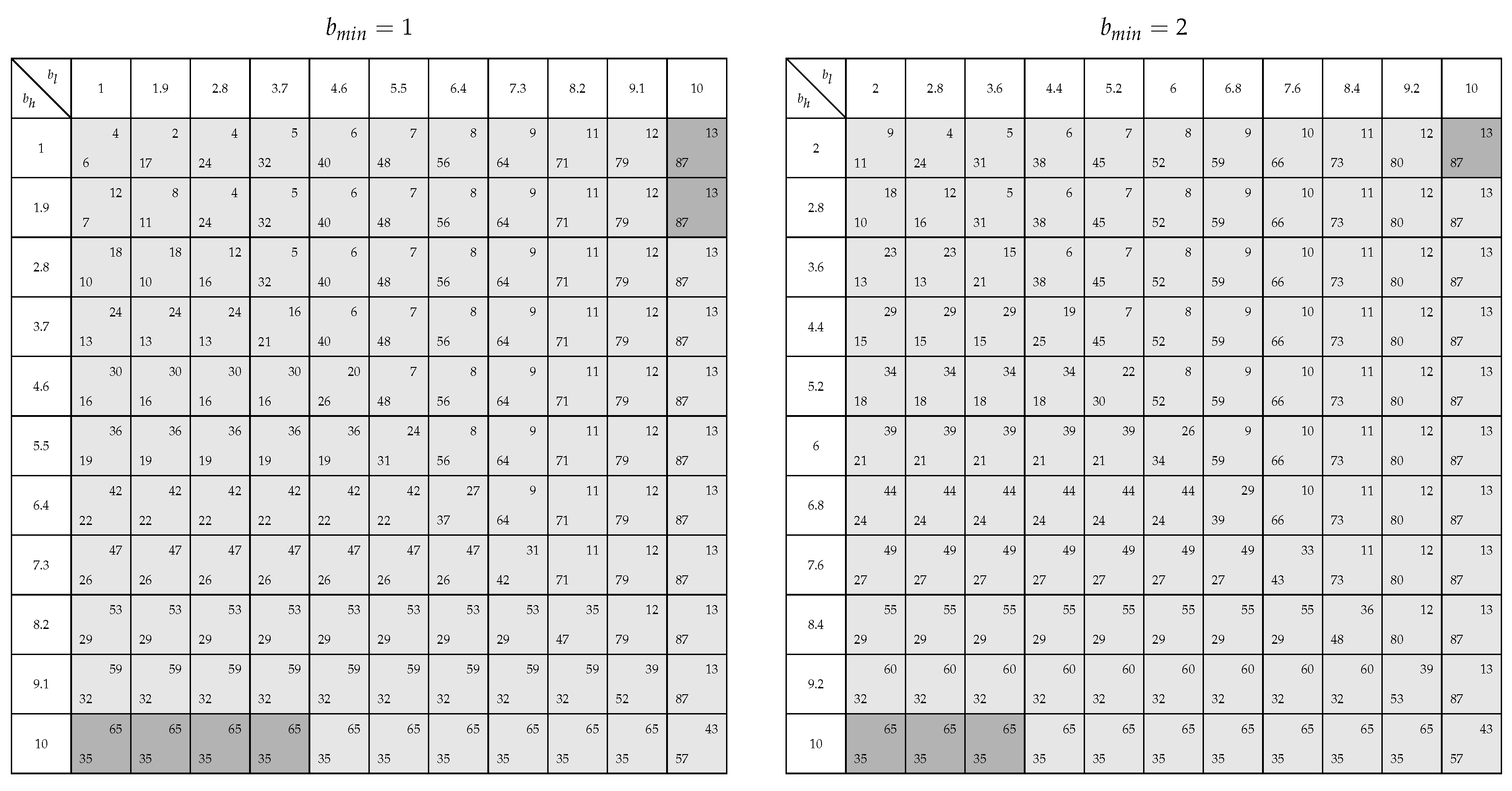
To illustrate the theoretical results, in Figure A4 we work out the players’ payoff using Equation (2). As can be observed in that figure, for the parameters defined in this game, , , , , , , there exist six equilibria in pure strategies. In four of those equilibria, the player with the higher production capacity, player h, submits the maximum bid, and player l submits a bid that makes undercutting unprofitable. In the other two equilibria, it is the player with the lower production capacity, player l, that submits the maximum bid.
As can be observed in the payoff matrix, each player prefers to play one of the equilibria in which the other player submits the maximum bid allowed by the auctioneer. In this appendix, we focus our analysis on the equilibrium selected by the tracing procedure method, the robustness to strategic uncertainty method, and the quantal response method. For a detailed review of the equilibrium selected using behavioural economics methods and for a complete analysis of the equilibrium selected using a lab experiment, see [4].
Tracing procedure method.
In the example that we use in this section, we increase the number of bids that the players can play from to . We do that because in the equations used in Lemma A1 and Propositions A1, A2, and A3, we assume that the expected payoff function (Equation (A1)) used by the players is almost continuous. Therefore, when the number of bids is low, the results using the raw information from the payoff matrices and the closed-form solutions differ slightly. In contrast, when the number of bids is large enough (N = 110), the results are the same.
To work out the graph presented in Figure 4, we use four different approaches.
In the first approach, we use the theoretical results presented in Propositions A1 and A2. According with those results, when , both players submit the minimum bid. When t increases, the player with the higher production capacity, player h, deviates first. By using this theoretical prediction, we fix player l’s strategy, assuming that it always plays the minimum bid. Then, we use Equation (4) to work out player h’s payoff, and for each t, we work out player h’s best strategy.
In the second approach, we work out the payoff matrix for each t using the payoff function of the original game defined in Equation (2) and the expected payoff defined in Equation (A1). Then, we develop an algorithm to work out the Nash equilibrium for each . The value of t obtained using the previous algorithm is summarized in column in Table A1. In that column, we work out the value t for which the players select the equilibrium defined by the first two columns in Table A1. Moreover, the pair of strategies for each t is the same for approaches 1 and 2. That information is summarized in Figure 4.
In the third approach, we find the value by implicitly solving Equation (A22). To solve this equation, we use the routine “fminsearch” in Matlab (version R2022; MathWorks, Natick, MA, USA). Those results are in column in Table A1. Finally, in the fourth approach, we use the closed-form solutions in Equations (A7) and (A11). Those results are summarized in column in Table A1.
As can be observed in that table, the value of t that we obtain using the four different approaches is almost the same.

Table A1.
t parameter using different methods. , , , , , , .
| m | M | (Nash Equilibrium) | (Fminsearch) | (Equations (A7) and (A11)) | ||
|---|---|---|---|---|---|---|
| 3.72 | 1 | 34 | 35 | 0.2330 | 0.2356 | 0.2409 |
| 4.63 | 1 | 45 | 46 | 0.261 | 0.2647 | 0.2679 |
| 5.54 | 1 | 56 | 57 | 0.2870 | 0.2901 | 0.2931 |
| 6.44 | 1 | 67 | 68 | 0.31 | 0.3138 | 0.3165 |
| 7.35 | 1 | 78 | 79 | 0.3330 | 0.3359 | 0.3385 |
| 8.26 | 1 | 89 | 90 | 0.3540 | 0.3566 | 0.3591 |
| 9.17 | 1 | 100 | 101 | 0.3740 | 0.3762 | 0.3784 |
| 10 | 1 | 109 | 110 | 0.39 | 0.3929 | 0.3934 |
Robustness to strategic uncertainty method.
To find the equilibrium selected by the robustness to strategic uncertainty method, it is necessary to work out the best response functions for each player. In this section, we explain the algorithm that we use to work out those functions.
First, since we know that follows a normal distribution (N ), we create random values drawn from a (N ).
Second, we set a value of . For that particular value, we set a value of , and for each pair , we work out the value .
Third, we compare the value with each of the points extracted from the normal distribution (N ) worked out in the first step. We count the values that are lower and higher than . Those values are the cumulative distribution values and in Equation (7).
Fourth, with the values , , , and , and knowing if or if , we can use Equation (7) to work out the expected value for every given a specific .
Fifth, given a specific , we find the value that maximizes player h’s expected value.
Sixth, we repeat the process for every and we obtain player h’s best response function (Figure 5).
Seventh, we repeat steps one to six to obtain player l’s best response function.
Quantal response method.
We describe in detail how we calculate the quantile response equilibria presented in Section 5 of the main text.
Define an increasing sequence of parameters such that and initialize .21 Then,
- For h, set to .
- Given , define a system of equations given by .
- Define optimization starting parameterswhere s is the number of pure strategies. Using , solve the system of equations given in step 2 to find .22
- If , set and go to step 1.23
One issue in numerically solving the system of equations given in step 2 is that as , we also have that . Even for relatively small values of , this can cause a numerical overflow. This is despite the probability being well-defined and bounded. To overcome this issue, we calculate the probabilities using an alternative representation of the LogSumExp function.
First, we have that for an n-dimensional vector, the LogSumExp function is defined as
Cao et al Ref. [21] note that this function can equivalently be written as
where .
From before, we have
Assuming that the probability of each strategy is strictly greater than zero, , we can rewrite this probability as
and replacing with , we have that
where . Using this form, we avoid numerical overflow and are able to find solutions for large values of .
Appendix C
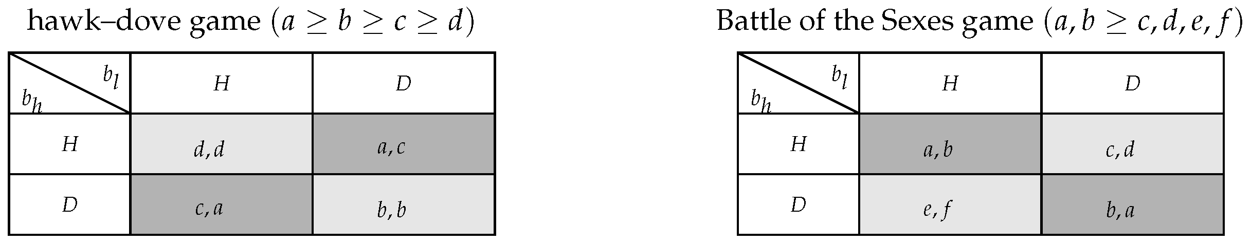
There appears to be no clear consensus in the literature as to the definition and the relationship between “hawk–dove” and “Battle-of-Sexes” games. According to [15], the Battle of the Sexes game defined in [18] and the hawk–dove game defined in [19] are equivalent. However, the payoff matrix in [7] (left-hand panel, Figure A5) and the one in [20] (right-hand panel, Figure A5) show that those games are different. Moreover, [22] study the hawk–dove and the Battle of the Sexes games, but the matrix that they present to characterize the hawk–dove game does not coincide with the one in [7]. In this paper, we assume that a game has the structure of a hawk–dove game when it follows the structure presented in [7].
When the auction is discriminatory, the tie-breaking rule is very important, since, in this case, the tie-breaking rule guarantees the existence of an equilibrium [14,17,23,24,25]. In particular, in the presence of positive marginal costs, the equilibrium only exists if, in the case of a tie, the most efficient supplier is dispatched first in the auction.
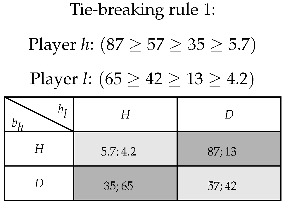
To study the importance of the tie-breaking rule for the equilibrium of a uniform-price auction, we take an example from Bigoni and Le Coq [26], and we apply the tie-breaking rules used in the literature on discriminatory-price auctions and in uniform-price auctions. In doing so, we can compare the impact of those tie-breaking rules on uniform-price auctions. We study the impact of five different tie-breaking rules on the equilibrium in a uniform-price auction.
To work out the payoff in the five tie-breaking rules implemented in this appendix, we use Equation (2) but modify the tie-breaking rule. When a marginal cost is introduced, that marginal cost must be taken into consideration while applying this equation.
Figure A5.
Generalized hawk–dove and Battle of the Sexes payoff matrices.

Tie-breaking rule 1: The suppliers are dispatched in proportion to their production capacities. This is the tie-breaking rule used in our paper. By using the parameters in Bigoni and Le Coq [26], we have that , , , , (Figure A6). That game has the structure of a “hawk–dove” game [7].
Figure A6.
Tie-breaking rule 1: Suppliers dispatched in proportion to their production capacities. Parameters: , , , , .
Figure A6.
Tie-breaking rule 1: Suppliers dispatched in proportion to their production capacities. Parameters: , , , , .

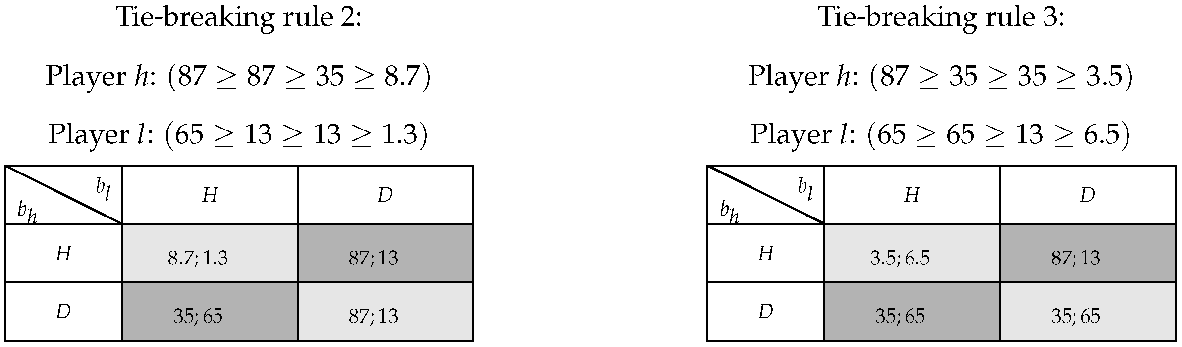
Tie-breaking rule 2: The larger supplier is dispatched first. By using the parameters in Bigoni and Le Coq [26], we have that , , , , (left-hand panel, Figure A7). That game has the structure of a “hawk–dove” game [7].
Tie-breaking rule 3: The smaller supplier is dispatched first. By using the parameters in Bigoni and Le Coq [26], we have that , , , , (right-hand panel, Figure A7). That game has the structure of a “hawk–dove” game [7].
Figure A7.
Tie-breaking rule 2: The larger supplier is dispatched first. Parameters: , , , , . Tie-breaking rule 3: The smaller supplier is dispatched first. Parameters: , , , , .
Figure A7.
Tie-breaking rule 2: The larger supplier is dispatched first. Parameters: , , , , . Tie-breaking rule 3: The smaller supplier is dispatched first. Parameters: , , , , .

When applying the previous tie-breaking rules (1–3), we assumed that the marginal costs are zero. As we have described above, the tie-breaking rule plays a crucial role in discriminatory-price auctions [14,17,23,24,25]. To study the impact of these tie-breaking rules on the equilibrium in the uniform-price auction, we now introduce positive marginal costs.
Tie-breaking rule 4: The efficient supplier is dispatched first (the efficient supplier is also the larger supplier). When the auction is discriminatory, this tie-breaking rule guarantees the existence of an equilibrium [14,17,23,24,25]. By using the parameters in Bigoni and Le Coq [26], we have that , , , , , , (right-hand panel, Figure A8). That game has the structure of a “hawk–dove” game [7].
Tie-breaking rule 5: The efficient supplier is dispatched first (the efficient supplier is also the smaller supplier). When the auction is discriminatory, this tie-breaking rule guarantees the existence of an equilibrium [14,17,23,24,25]. By using the parameters in Bigoni and Le Coq [26], we have that , , , , , , (right-hand panel, Figure A8). That game has the structure of a “hawk–dove” game [7].
Figure A8.
Tie-breaking rule 4: The efficient supplier is dispatched first (the efficient supplier is also the larger supplier). Parameters: , , , , , , . Tie-breaking rule 5: The efficient supplier is dispatched first (the efficient supplier is also the smaller supplier). Parameters: , , , , , , .
Figure A8.
Tie-breaking rule 4: The efficient supplier is dispatched first (the efficient supplier is also the larger supplier). Parameters: , , , , , , . Tie-breaking rule 5: The efficient supplier is dispatched first (the efficient supplier is also the smaller supplier). Parameters: , , , , , , .

As can be observed above, irrespective of the tie-breaking rule, the uniform-price auction has the structure of a “hawk–dove” game following [7]. Given that a clear consensus does not appear to exist in the literature about the definition and the relationship between “hawk–dove” and “Battle-of-Sexes” games, the analysis in our paper contributes to fostering research on the comparison between these two types of games and to analyzing which equilibrium emerges.
| 1 | We frame the paper as a uniform-price auction because we are interested in studying the strategic behaviour of firms in an industrial organization context. However, there are many other real examples such as trade wars, military battles, collective bargaining, and legal disputes—of which the hawk–dove game is the prototypical example. |
| 2 | As we have pointed out in note 1, we frame the analysis as an industrial organization problem. However, by using an experiment, Ref. [4] study a similar hawk–dove game framing the asymmetries as the relative strength of the players. In that sense, their outline is more clean, since they need a neutral framing to avoid any possible setting-induced bias in the players’ behaviour during the experiment. |
| 3 | The inelastic demand assumption is not a critical one, but it simplifies the analysis. When the demand is elastic, the set of strategies changes, since the maximum bid is determined by the bid that maximizes the residual demand profit function. When the demand is elastic, the rationing rule plays a crucial role in determining the profitability of the residual demand profit function, and therefore, defining the maximum bid set in the auction. Moreover, the rationing rule could also foster or hinder the coordination in one of the equilibria. A complete discussion of the role of the rationing rule determining the equilibrium in models of price competition with elastic demand can be found in [5,6]. |
| 4 | We provide a complete description of the uniform-price auction in the model section and in Appendix C. In Appendix C, we explain that with the tie-breaking rule implemented in the uniform-price auction, the uniform-price auction has the structure of a “hawk–dove” game as defined in [7]. In this appendix, we also discuss the relationship between the “hawk–dove” and the “Battle-of-Sexes” games and work out the equilibrium in a uniform-price auction when five different tie-breaking rules are implemented. |
| 5 | We believe that our assumptions are less stringent, since we are not imposing any restriction on the set of strategies that the players can select. This assumption is validated by experimental evidence [4], where the authors find that the players select strategies outside the set of Nash equilibrium strategies. Moreover, by not restricting the set of strategies, we follow the same approach as in the robustness to strategic uncertainty method [2] and quantal response method [3], making the predictions of the three theoretical methods comparable. |
| 6 | As we have presented in note 2, in [4], the inequalities represent the relative strength of the players. |
| 7 | The minimum bid in the auction () and the maximum bid () are determined by the auctioneer. The minimum bid guarantees a minimum profit for the players. The maximum bid represents the reservation price for the consumers of the good. |
| 8 | It is important to emphasize that is only valid under the assumption that . When , is slightly different, since in this case both players have enough production capacity to satisfy the entire demand and the equilibrium is unique. For a complete analysis of the uniform-price auction when the demand is low, see [17]. |
| 9 | The profit function in Equation (2) follows the classical profit function definition in a uniform-price auction [17]. In Section 3, Section 4 and Section 5, we define other profit functions following the definitions of [4] that we are studying. To avoid confusion, we formally define these functions when we apply them. |
| 10 | As with , is slightly different when the assumptions of the model are relaxed. |
| 11 | There appears to be no clear consensus in the literature as to the the definition and relationship between “hawk–dove” and “Battle-of-Sexes” games. According to [15], the Battle of the Sexes game defined in [18] and the hawk–dove game defined in [19] are equivalent. However, the payoff matrix in [7] and the one in [20] show that those games are different. In this paper, we assume that a game has the structure of a hawk–dove game when it follows the structure presented in [7]. In Appendix C, we apply five different tie-breaking rules to the uniform-price auction, and we show that for the applied tie-breaking rules, the uniform-price auction has the structure of a “hawk–dove” game as defined in [7]. For a complete discussion, we refer the reader to Appendix C. |
| 12 | |
| 13 | As we have discussed in the model section, the number of bids can be arbitrary large by raising N. When the number of bids tends to infinity, the weight of the payoffs in the diagonal tend to zero and can be “neglected” when equilibrium selection techniques are applied. |
| 14 | We restrict our attention to the low-demand case, since when the demand is intermediate or high, an increase in the lower bid does not affect the equilibrium selected by the tracing procedure. |
| 15 | |
| 16 | In this section, we have changed slightly the original notation in [3], since in our paper we use to denote players’ profits, while in their paper they denote those profits as . We made that change to help the reader compare the three methods that we are studying by having a coherent notation through the paper. It is also important to note that in the quantal response method, the subindexes i and j refer to the strategies, and not to the players. |
| 17 | It is important to note that our results, as are those of [3], are based on numerical simulations. In our case, the numerical simulations presented in Figure 6 are based on the two matrices introduced in Appendix B, Figure A4, which are the matrices that we have used in all the numerical examples in the paper. |
| 18 | |
| 19 | We assume that N is large. This guarantees that the first and second derivatives of adequately approximate the change in payoffs as players adjust their strategy slightly and the probability of a tie goes to 0, so that does not have a term for that possibility. |
| 20 | |
| 21 | Choosing to be roughly zero helps find good starting values for subsequent values of as we have that when , each strategy is played with equal probability. |
| 22 | We use Matlab’s non-linear equation solver fsolve, with function and x tolerances both set to 10 × 10−10. |
| 23 | An alternative termination criteria is to look at the distance between and . In our application, we define our sequence such that the are increasing exponentially rather than linearly and choose therefore to terminate at a large predefined . |
References
- Harsanyi, J.; Selten, R. A General Theory of Equilibrium Selection in Games; The MIT Press: Cambridge, MA, USA, 1988. [Google Scholar]
- Andersson, O.; Argenton, C.; Weibull, J. Robustness to Strategic Uncertainty. Games Econ. Behav. 2014, 85, 272–288. [Google Scholar] [CrossRef]
- McKelvey, R.; Palfrey, T.R. Quantal Response Equilibria for Normal Form Games. Games Econ. Behav. 1998, 10, 6–38. [Google Scholar] [CrossRef]
- de Paz, M.; Bigoni, M.; Le Coq, C. Beyond Hawks and Doves: Can Inequality Ease Coordination? CEPR: Paris, France, 2022. [Google Scholar]
- Allen, B.; Hellwig, M. Bertrand-Edgeworth Duopoly with Proportional Residual Demand. Int. Econ. Rev. 1993, 34, 39–60. [Google Scholar] [CrossRef]
- Davidson, C.; Deneckere, R. Long-Run Competition in Capacity, Short-Run Competition in Price, and the Cournot Model. Rand J. Econ. 1986, 17, 404–415. [Google Scholar] [CrossRef]
- Benndorf, V.; Martínez-Martínez, I.; Normann, H.-T. Equilibrium Selection with Couple Populations in hawk–dove Games: Theory and Experiment in Continuous Time. J. Econ. Theory 2016, 165, 472–486. [Google Scholar] [CrossRef]
- Boom, A. Equilibrium Selection with Risk Dominance in a Multiple-Unit Unit Price Auction; Working Paper; 2008; Available online: https://ideas.repec.org/p/hhs/cbsnow/2008_002.html (accessed on 20 October 2023).
- van Damme, E.; Hurkens, S. Endogenous Stackelberg Leadership. Games Econ. Behav. 1999, 28, 105–179. [Google Scholar] [CrossRef]
- Endogenous timing in duopoly games: Stackelberg or cournot equilibria. Games Econ. Behav. 1990, 1, 29–46.
- van Damme, E.; Hurkens, S. Endogenous Price Leadership. Games Econ. Behav. 2004, 47, 404–420. [Google Scholar] [CrossRef]
- Canoy, M. Product Differentiation in a Bertrand—Edgeworth Duopoly. J. Econ. Theory 1996, 70, 158–179. [Google Scholar] [CrossRef]
- Deneckere, R.J.; Kovenock, D. Price Leadership. Rev. Econ. Stud. 1992, 59, 143–162. [Google Scholar] [CrossRef]
- Osborne, M.J.; Pitchik, C. Price Competition in a Capacity-Constrained Duopoly. J. Econ. Theory 1986, 38, 238–260. [Google Scholar] [CrossRef]
- Cabrales, A.; García-Fontes, W.; Motta, M. Risk Dominance Selects the Leader: An Experimental Analysis. Int. J. Ind. Organ. 2000, 18, 137–162. [Google Scholar] [CrossRef]
- Allan, B.B. Social Action in Quantum Social Science. Millenn. J. Int. Stud. 2018, 47, 87–98. [Google Scholar] [CrossRef]
- Fabra, N.; von der Fehr, N.H.; Harbord, D. Designing Electricity Auctions. Rand J. Econ. 2006, 37, 23–46. [Google Scholar] [CrossRef]
- Luce, R.; Raiffa, H. Games and Decisions; Wiley: New York, NY, USA, 1957. [Google Scholar]
- Binmore, K. Fun and Games; D.C. Health: Lexington, MA, USA, 1992. [Google Scholar]
- Belleflamme, P.; Peitz, M. Industrial Organization. In Markets and Strategies; Cambridge University Press: Cambridge, UK, 2015. [Google Scholar]
- Gao, B.; Pavel, L. On the Properties of the Softmax Function with Application in Game Theory and Reinforcement Learning. Working Paper. arXiv 2018, arXiv:1704.00805. Available online: https://arxiv.org/abs/1704.00805 (accessed on 28 October 2023).
- Tirole, J.; Fudenberg, D. Game Theory; MIT Press: Cambridge, MA, USA, 1991. [Google Scholar]
- Blázquez, M. Electricity Auctions in the Presence of Transmission Constraints and Transmission Costs. Energy Econ. 2018, 74, 605–627. [Google Scholar] [CrossRef]
- Dasgupta, P.; Maskin, E. The Existence of Equilibrium in Discontinuous Economic Games, II: Applications. Rev. Econ. Stud. 1986, 53, 27–41. [Google Scholar] [CrossRef]
- Deneckere, R.; Kovenock, D. Bertramd-Edgeworth Duopoly with Unit Cost Asymmetry. Econ. Theory 1996, 8, 1–25. [Google Scholar] [CrossRef]
- Bigoni, M.; Le Coq, C. Beyond Hawks and Doves: Can Inequality Ease Coordination? 2023. Available online: https://cepr.org/publications/dp17867 (accessed on 25 October 2023).
Figure 1.
Set of strategies.

Figure 2.
Demand thresholds for players h, l.

Figure 3.
Expected payoffs , , , , .

Figure 4.
Tracing procedure method , , , .

Figure 5.
Players’ best response functions (, , , , ).

Figure 6.
Quantal response method (, , , , ).

Disclaimer/Publisher’s Note: The statements, opinions and data contained in all publications are solely those of the individual author(s) and contributor(s) and not of MDPI and/or the editor(s). MDPI and/or the editor(s) disclaim responsibility for any injury to people or property resulting from any ideas, methods, instructions or products referred to in the content. |
© 2023 by the authors. Licensee MDPI, Basel, Switzerland. This article is an open access article distributed under the terms and conditions of the Creative Commons Attribution (CC BY) license (https://creativecommons.org/licenses/by/4.0/).
Share and Cite
MDPI and ACS Style
Blázquez de Paz, M.; Koptyug, N. Equilibrium Selection in Hawk–Dove Games. Games 2024, 15, 2. https://doi.org/10.3390/g15010002
AMA Style
Blázquez de Paz M, Koptyug N. Equilibrium Selection in Hawk–Dove Games. Games. 2024; 15(1):2. https://doi.org/10.3390/g15010002
Chicago/Turabian StyleBlázquez de Paz, Mario, and Nikita Koptyug. 2024. "Equilibrium Selection in Hawk–Dove Games" Games 15, no. 1: 2. https://doi.org/10.3390/g15010002
Note that from the first issue of 2016, this journal uses article numbers instead of page numbers. See further details here.