
Generalized Hyperbolic Discounting in Security Games of Timing

Abstract
:1. Introduction
2. Related Work
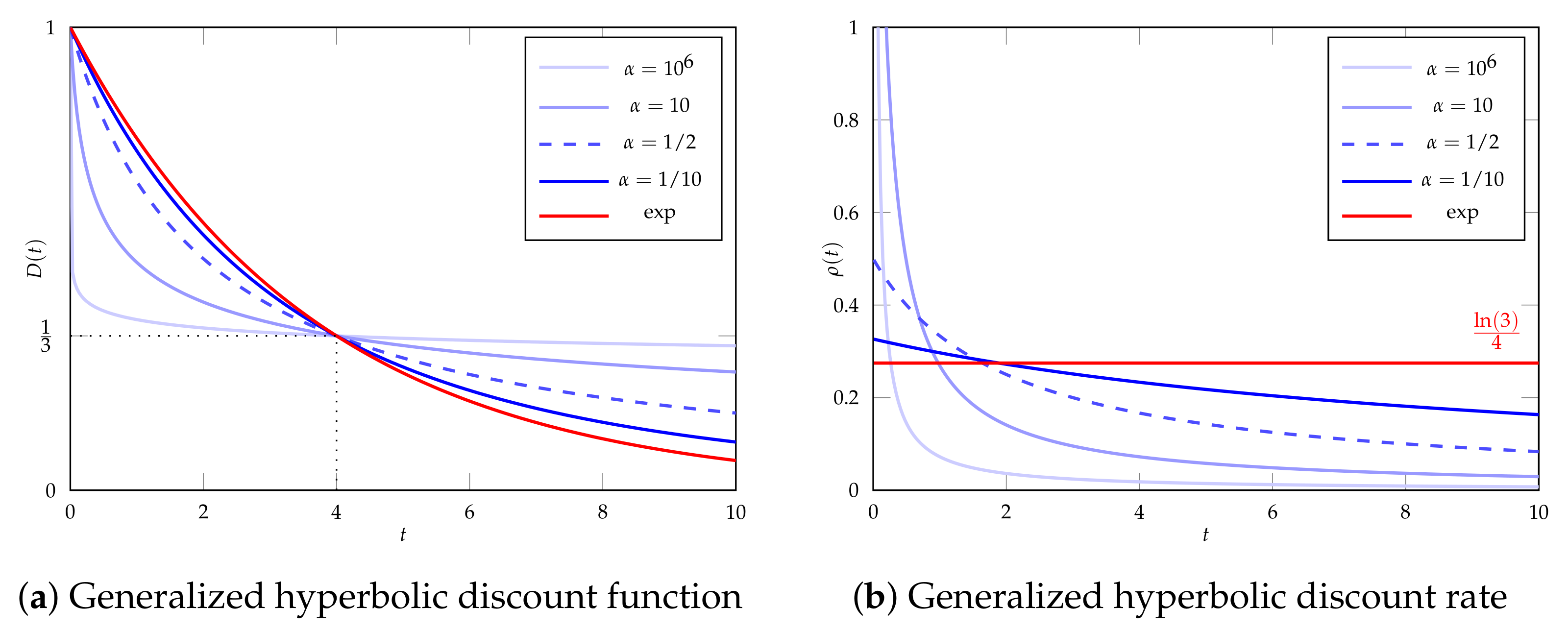
3. Discounting
- For (super-hyperbolic discounting), the area under ’s curve is finite and given by:
- For (sub-hyperbolic discounting), does not converge for .
4. Model
4.1. Overview
4.2. Player Strategies
4.3. Player Control
4.4. Player Utilities
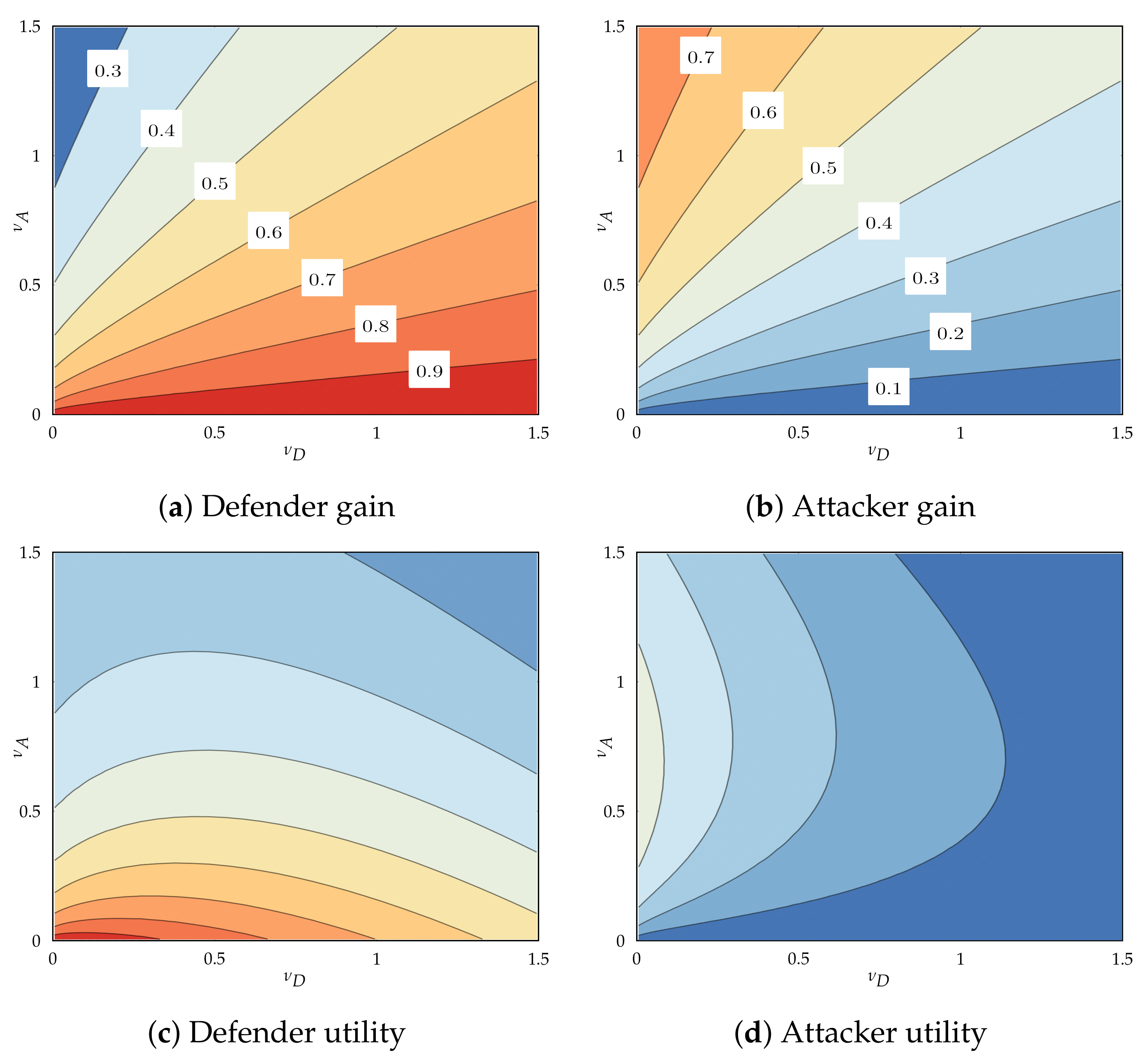
4.4.1. Gains
4.4.2. Costs
4.5. Restricted Strategies
4.5.1. Exponential Strategies
4.5.2. Periodic Strategies with Random Phase
5. Analysis
5.1. Sub-Hyperbolic Discounting
5.2. Super-Hyperbolic Discounting
5.3. Player Utilities for Super-Hyperbolic Discounting
5.3.1. For Exponential Play
5.3.2. For Periodic Play
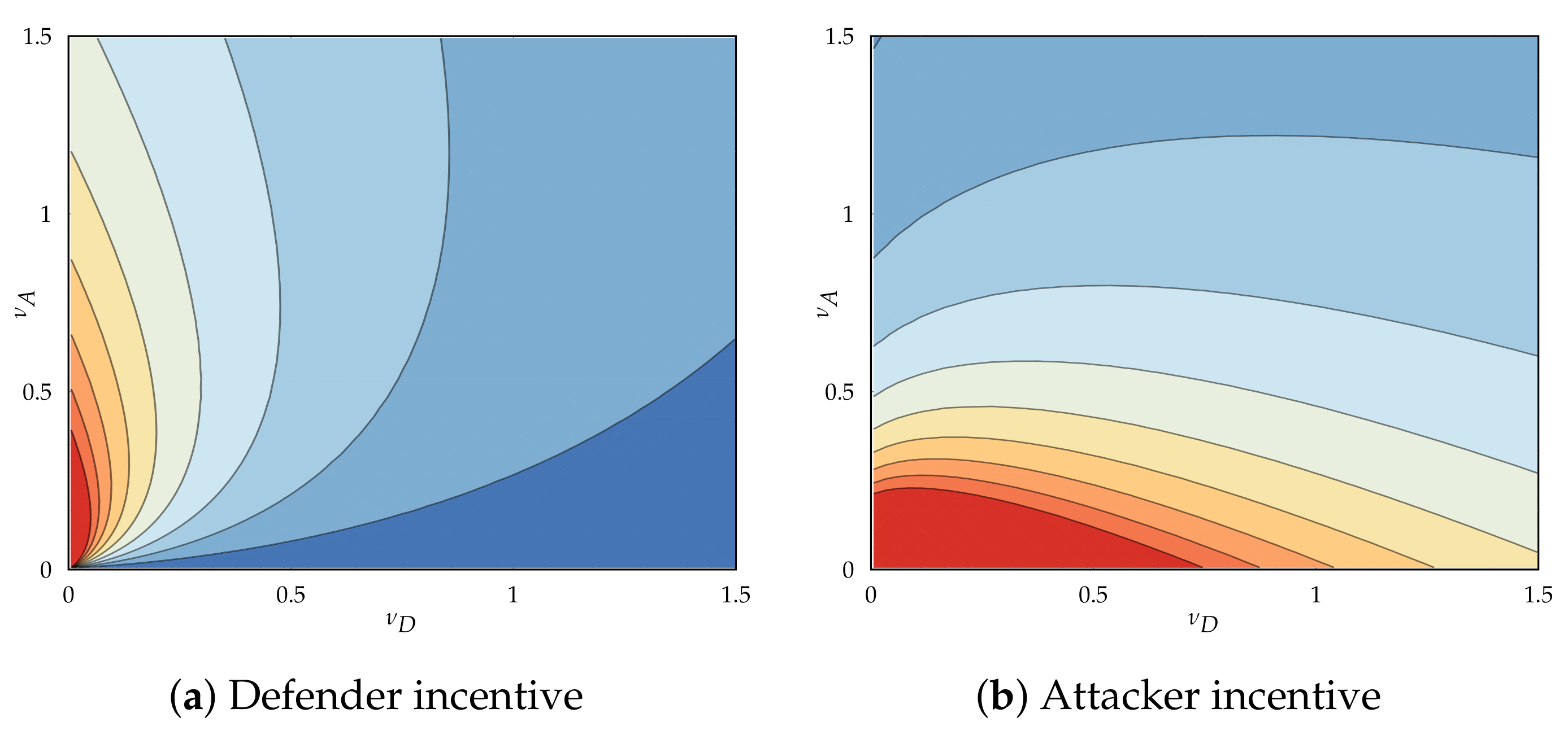
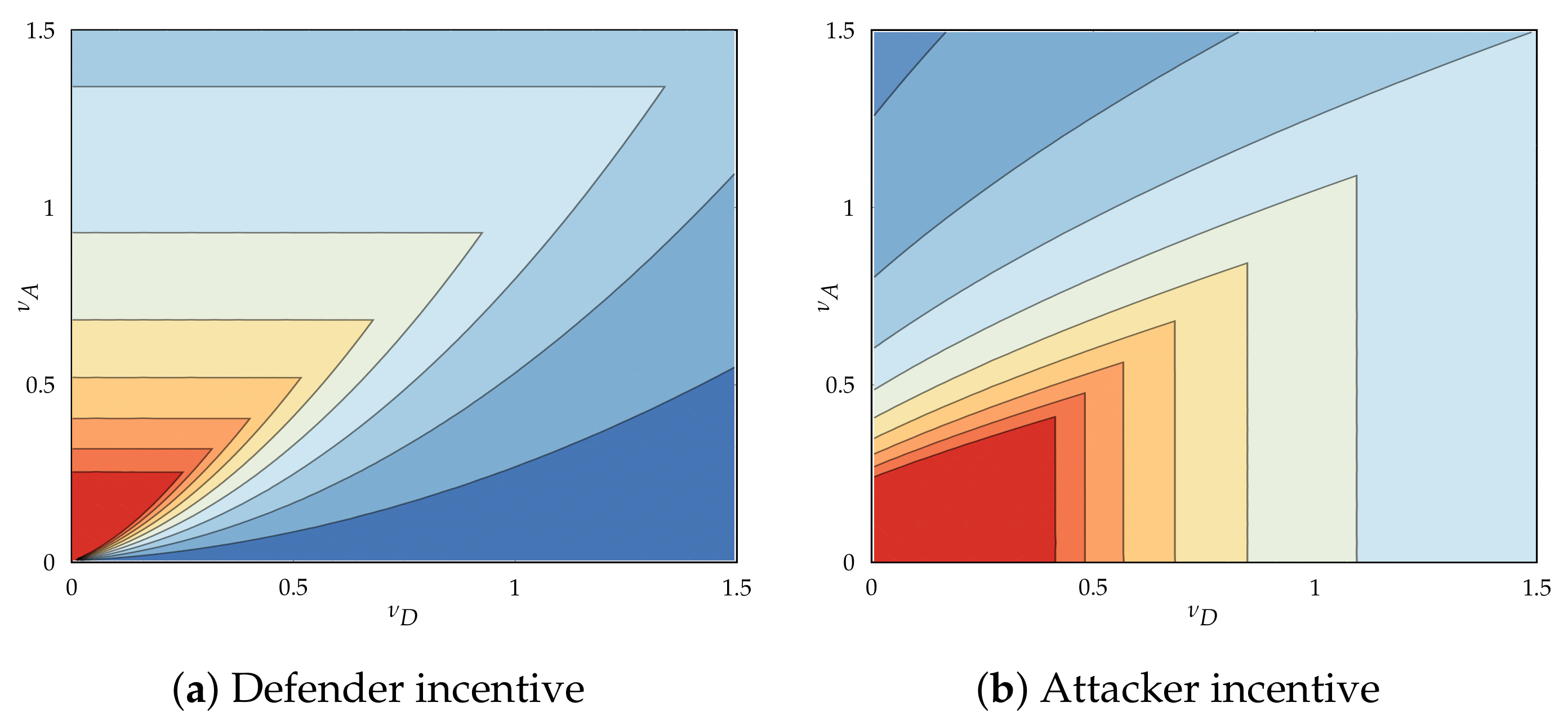
5.4. Player Incentives and Best Responses
5.4.1. Directionality of Incentives and Base Incentive
- If her base incentive is negative, her best response is not to play.
- If her base incentive is strictly positive, then her incentive function has a single root at , and her best response is to play at rate .
- If her base incentive is strictly negative, then her unique best response is not to play.
- If her base incentive is zero, then any play rate is a best response.
- If her base incentive is strictly positive, then her incentive function has a single root at , and her best response is to play at rate .
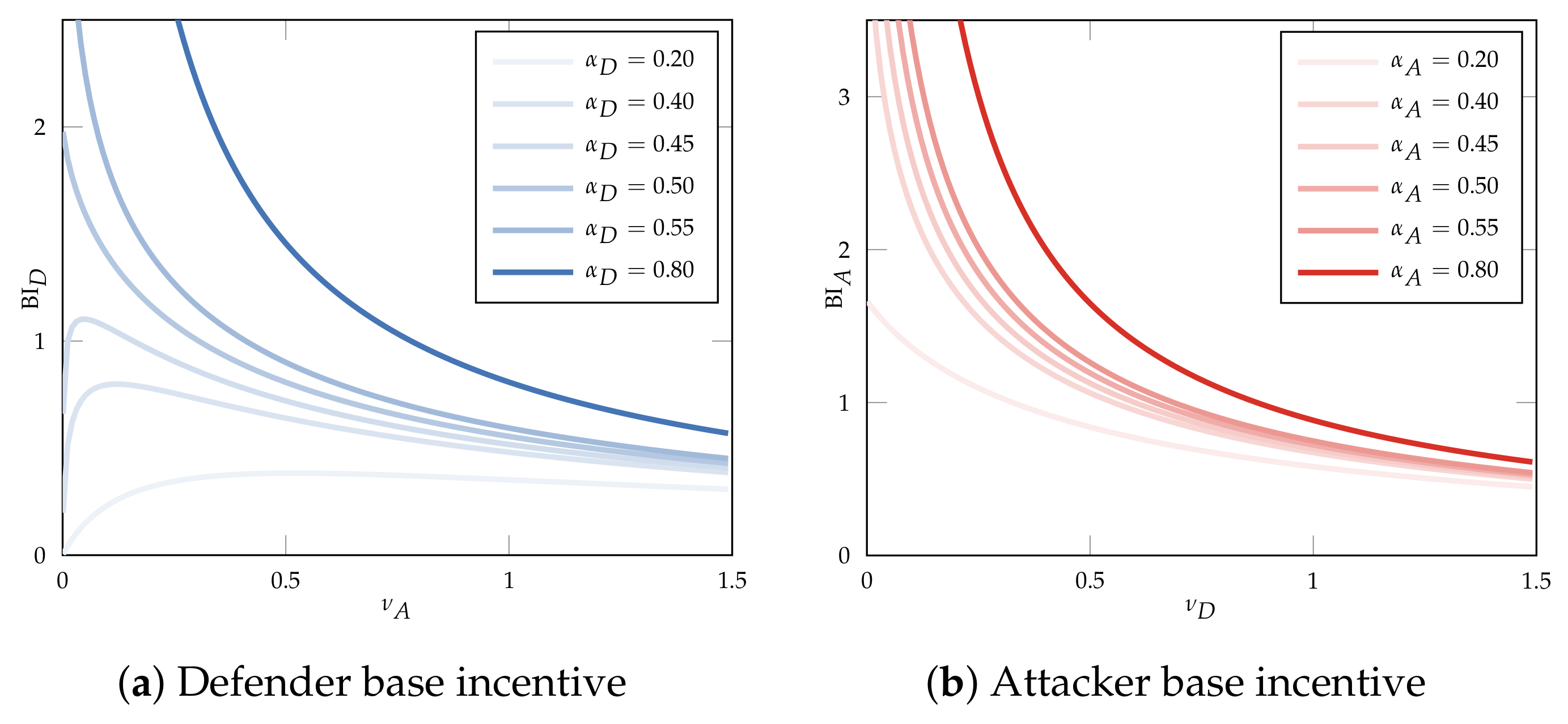
5.4.2. Directionality and Origin of Base Incentive
- If , move at non-zero rates, regardless of cost ().
- If , move at non-zero rates iff and at the zero rate otherwise.
5.5. Equilibria for Super-Hyperbolic Discounting
5.5.1. Non-Participatory Equilibria
- If and , then there is a non-participatory equilibrium in which neither player moves.
- Otherwise, there may be an equilibrium in which only the attacker plays if or if and .
| Algorithm 1 Procedure for finding the set of non-participatory equilibria for exponential and periodic play |
|
5.5.2. Participatory Equilibria for Exponential Play
- , where is the (unique) root of the attacker’s base incentive function.
- If , then , where is the root of the defender’s base incentive function.
- If , then , where and are the roots of the defender’s base incentive function with .
5.5.3. Participatory Equilibria for Periodic Play
| Algorithm 2 Algorithm for finding the set of participatory equilibria with faster-moving defender for periodic play |
// Check if the attacker’s base incentive has a root
|
6. Discussion
6.1. Degenerated Discounting Behavior
- All existing research and results on FlipIt-like timing games without discounting carry over to the most commonly observed discounting behavior. This includes the results presented in van Dijk et al. [2] and follow-up work without discounting.
- The players’ utilities, incentives, best responses, and the game’s equilibria are not impacted by the fact that the defender starts the game in control of the resource. Differences between defender and attacker emerge only when discounting super-hyperbolically.
Commitment
Organizational Actors
Rationalization of Risk
6.2. Short-Horizon and Long-Horizon Discounting
6.3. Player Indifference for Periodic Play
6.4. Effective Move Cost and Motivation
- Increased effective cost. Players must pay for the instantaneous cost of a move “up front”. They first pay for the move and accrue benefits from this move later, resulting in the benefits being discounted at a higher rate than the costs. For both players, this effect results in a slightly higher “effective cost” of a move and reduces their incentive.
- Relevance of starting position. Another behavioral change is caused by the defender starting out in control of the resource. This envigorates the attacker—he will attack at reasonably high rates to reduce the time before the first move to obtain the resource before its value has been discounted away, even in the absence of a defender. In contrast, this demotivates the defender, as she is sure to be in control of the resource when it is at its most valuable.
6.5. Equilibrium Selection
- The attacker moves infrequently, and the defender does not respond.
- Both players move at a low, non-zero rate.
- Both players move at a higher, non-zero rate.
6.6. Perfectly Secure Systems
6.7. Non-Optimality of Periodic Strategies
7. Conclusions
Author Contributions
Funding
Data Availability Statement
Conflicts of Interest
Appendix A. Divergent Behavior
Appendix A.1. Gains
- ,
- ,
- .
Appendix A.2. Costs
Appendix B. Player Gains
Appendix B.1. Structural Aspects
Appendix B.2. Exponential Play
Appendix B.3. Periodic Play
Appendix C. Player Incentives
Appendix C.1. Expressions
Appendix C.1.1. Exponential Play
Appendix C.1.2. Periodic Play
Appendix C.2. Direction of Incentive
Appendix C.2.1. Exponential Play
- The exponential integral function is positive:
- The exponential integral function is decreasing in its order r, that is, the partial derivative of to r is negative and
- The rate at which the decrease happens is decreasing in the order r, that is, the second-order partial derivative of to r is positive and consequently
Appendix C.2.2. Periodic Play
- If she is the slower-moving player, her incentive is independent of her play rate.
- If she is the faster-moving player, her incentive is strictly decreasing in her play rate.
Appendix C.3. Base Incentives
- The attacker’s base incentive function is strictly decreasing.
- If , then the defender’s base incentive function is strictly decreasing for strictly positive attack rates ().
- If , then the defender’s base incentive function is first strictly increasing, then strictly decreasing.
Appendix C.4. Origin of Base Incentive
- It is equal to for .
- If , then it becomes unboundedly large for .
- If , then it is equal to for .
- If , then it is equal to for .
- If , then it becomes unboundedly large for .
- If , then it is equal to for .
Appendix D. A Renewal Strategy Beating the Periodic Strategy
| 1 | |
| 2 | In Merlevede et al. [13], these parameters are named and instead of and , and and instead of and . |
| 3 | A player can move at most once at a particular instance of time and a finite number of times over any finite time interval. |
| 4 | We limit ourselves to cases where both players discount super-hyperbolically and do not exhaustively cover scenarios where one player discounts super-hyperbolically and another sub-hyperbolically. As there is no discontinuity in player best responses near , outcomes for mixed scenarios can be observed under the super-hyperbolic discounting by bringing and close to each other. |
| 5 | This research does primarily focus on income or costs occurring at one particular point in time, not on continuous income and cost streams as is the case here. |
| 6 | We pick a value for and then compute parameters and as and . |
| 7 | Define income resulting from a move as follows: (•) When a player in control of the resource performs a move, it does not result in income. (•) When a player not in control of the resource performs a move, flipping the resource, it results in income equal to the value generated by the resource from the time of the move until the resource flips again. Start by splitting the game into two parts: the part of the game before the attacker’s first move (ante) and the part after the attacker’s first move (post). • (ante) If the attacker is the slower player, this part of the game always yields him precisely zero gain, irrespective of either player’s play rate. If the defender is the slower player, this part of the game does yield her gain, but the expected amount only depends on the duration of ante, which is also independent of her play rate. • (post) The probability density of the slower player flipping at any time is constant and equal to her play rate. Every one of her moves results in an expected income; while difficult to determine this income exactly, it is independent of her own play rate, as it is certain to result in a change of ownership while the value of ownership depends only on the time and the play rate of the faster player. The slower player’s gain is, therefore, proportional to her play rate, and her incentive is independent of her play rate. |
| 8 | To be precise, the periodic strategies strictly dominate the class of non-arithmetic or non-lattice renewal strategies. Arithmetic strategies are strategies for which all possible realizations happen at an integer multiple of some real number. |
| 9 | The CDF for the time of the first move is , where is the indicator function. The PDF for the time of the first move is its derivative, . An expression for the total anonymous gain is, therefore,
We can confirm that this expression is equal to the sum of and as presented in Lemmas A16 and A17. |
| 10 | The probability of the faster player having moved last at any point in time is equal to . The slower player moved last with probability . |
| 11 | The expected duration of the intervals owned by the faster-moving player is . The intervals of the slower-moving player have a shorter expected length of . |
| 12 | https://dlmf.nist.gov/8.19.E15, (accessed on 10 November 2023). |
References
- Radzik, T. Results and Problems in Games of Timing; Lecture Notes-Monograph Series; Institute of Mathematical Statistics: Durham, NC, USA, 1996; pp. 269–292. [Google Scholar] [CrossRef]
- van Dijk, M.; Juels, A.; Oprea, A.; Rivest, R.L. FlipIt: The Game of “Stealthy Takeover”. J. Cryptol. 2012, 26, 655–713. [Google Scholar] [CrossRef]
- Pawlick, J.; Farhang, S.; Zhu, Q. Flip the Cloud: Cyber-Physical Signaling Games in the Presence of Advanced Persistent Threats. In Decision and Game Theory for Security; Khouzani, M., Panaousis, E., Theodorakopoulos, G., Eds.; Number 9406 in Lecture Notes in Computer Science; Springer International Publishing: Cham, Switzerland, 2015; pp. 289–308. [Google Scholar] [CrossRef]
- Kushner, D. The Real Story of Stuxnet. IEEE Spectrum 2013, 50, 48–53. [Google Scholar] [CrossRef]
- Barrett, D.; Yadron, D.; Paletta, D. U.S. Suspects Hackers in China Breached about 4 Million People’s Records, Officials Say. Available online: http://www.wsj.com/articles/u-s-suspects-hackers-in-china-behind-government-data-breach-sources-say-1433451888 (accessed on 7 October 2023).
- Perez, E.; Prokupecz, S. U.S. Data Hack May Be 4 Times Larger Than the Government Originally Said. Available online: http://edition.cnn.com/2015/06/22/politics/opm-hack-18-milliion (accessed on 7 September 2023).
- Gallagher, R. The Inside Story of How British Spies Hacked Belgium’s Largest Telco. Available online: https://theintercept.com/2014/12/13/belgacom-hack-gchq-inside-story/ (accessed on 10 November 2023).
- Price, R. TalkTalk Hacked: 4 Million Customers Affected, Stock Plummeting, ‘Russian Jihadist Hackers’ Claim Responsibility. Available online: http://uk.businessinsider.com/talktalk-hacked-credit-card-details-users-2015-10 (accessed on 10 November 2023).
- Reuters. Premera Blue Cross Says Data Breach Exposed Medical Data. Available online: http://www.nytimes.com/2015/03/18/business/premera-blue-cross-says-data-breach-exposed-medical-data.html (accessed on 10 November 2023).
- ESET. APT Activity Report T2 2022. Available online: https://www.eset.com/int/business/resource-center/reports/eset-apt-activity-report-t2-2022 (accessed on 10 November 2023).
- Cole, E. (Ed.) Preface. In Advanced Persistent Threat; Syngress: Boston, MA, USA, 2013; pp. xv–xvi. [Google Scholar] [CrossRef]
- Nadela, S. Enterprise Security in a Mobile-First, Cloud-First World. Available online: http://news.microsoft.com/security2015/ (accessed on 10 November 2023).
- Merlevede, J.; Johnson, B.; Grossklags, J.; Holvoet, T. Exponential Discounting in Security Games of Timing. In Proceedings of the Workshop on the Economics of Information Security (WEIS), Boston, MA, USA, 2–3 June 2019. [Google Scholar]
- Merlevede, J.; Johnson, B.; Grossklags, J.; Holvoet, T. Exponential Discounting in Security Games of Timing. J. Cybersecur. 2021, 7, tyaa008. [Google Scholar] [CrossRef]
- Merlevede, J.; Johnson, B.; Grossklags, J.; Holvoet, T. Time-Dependent Strategies in Games of Timing. In Decision and Game Theory for Security; Alpcan, T., Vorobeychik, Y., Baras, J.S., Dán, G., Eds.; Number 11836 in Lecture Notes in Computer Science; Springer International Publishing: Cham, Switzerland, 2019; pp. 310–330. [Google Scholar] [CrossRef]
- Loewenstein, G.; Prelec, D. Anomalies in Intertemporal Choice: Evidence and an Interpretation. Q. J. Econ. 1992, 107, 573–597. [Google Scholar] [CrossRef]
- Samuelson, P. A Note on Measurement of Utility. Rev. Econ. Stud. 1937, 4, 155–161. [Google Scholar] [CrossRef]
- Ramsey, F.P. A Mathematical Theory of Saving. Econ. J. 1928, 38, 543–559. [Google Scholar] [CrossRef]
- Strotz, R.H. Myopia and Inconsistency in Dynamic Utility Maximization. Rev. Econ. Stud. 1955, 23, 165–180. [Google Scholar] [CrossRef]
- Koopmans, T.C. Stationary Ordinal Utility and Impatience. Econometrica 1960, 28, 287–309. [Google Scholar] [CrossRef]
- Fishburn, P.C.; Rubinstein, A. Time Preference. Int. Econ. Rev. 1982, 23, 677–694. [Google Scholar] [CrossRef]
- Callender, C. The Normative Standard for Future Discounting. Australas. Philos. Rev. 2021, 5, 227–253. [Google Scholar] [CrossRef]
- Vanderveldt, A.; Oliveira, L.; Green, L. Delay Discounting: Pigeon, Rat, Human—Does it Matter? J. Exp. Psychol. Anim. Learn. Cogn. 2016, 42, 141–162. [Google Scholar] [CrossRef]
- O’Donoghue, T.; Rabin, M. Doing It Now or Later. Am. Econ. Rev. 1999, 89, 103–124. [Google Scholar] [CrossRef]
- Laibson, D. A Cue-theory of Consumption. Q. J. Econ. 2001, 116, 81–119. [Google Scholar] [CrossRef]
- Zauberman, G.; Kim, B.K.; Malkoc, S.A.; Bettman, J.R. Discounting Time and Time Discounting: Subjective Time Perception and Intertemporal Preferences. J. Mark. Res. 2009, 46, 543–556. [Google Scholar] [CrossRef]
- Kahneman, D.; Tversky, A. Prospect Theory: An Analysis of Decision under Risk. Econometrica 1979, 47, 363–391. [Google Scholar] [CrossRef]
- Frederick, S. Cognitive Reflection and Decision Making. J. Econ. Perspect. 2005, 19, 25–42. [Google Scholar] [CrossRef]
- Laibson, D. Golden Eggs and Hyperbolic Discounting. Q. J. Econ. 1997, 112, 443–478. [Google Scholar] [CrossRef]
- Ericson, K.M.; Laibson, D. Chapter 1—Intertemporal Choice. In Handbook of Behavioral Economics—Foundations and Applications 2; Elsevier: Amsterdam, The Netherlands, 2019; pp. 1–67. [Google Scholar] [CrossRef]
- Herrnstein, R.J. Relative and Absolute Strength of Response as a Function of Frequency of Reinforcement. J. Exp. Anal. Behav. 1961, 4, 267–272. [Google Scholar] [CrossRef]
- McKerchar, T.L.; Green, L.; Myerson, J. On the Scaling Interpretation of Exponents in Hyperboloid Models of Delay and Probability Discounting. Behav. Process. 2010, 84, 440–444. [Google Scholar] [CrossRef]
- Myerson, J.; Green, L. Discounting of Delayed Rewards: Models of Individual Choice. J. Exp. Anal. Behav. 1995, 64, 263–276. [Google Scholar] [CrossRef]
- McKerchar, T.L.; Green, L.; Myerson, J.; Pickford, T.S.; Hill, J.C.; Stout, S.C. A Comparison of Four Models of Delay Discounting in Humans. Behav. Process. 2009, 81, 256–259. [Google Scholar] [CrossRef] [PubMed]
- Green, L.; Myerson, J.; Vanderveldt, A. Delay and Probability Discounting. In The Wiley Blackwell Handbook of Operant and Classical Conditioning; John Wiley & Sons, Ltd.: Hoboken, NJ, USA, 2014; Chapter 13; pp. 307–337. [Google Scholar] [CrossRef]
- Sozou, P.D. On Hyperbolic Discounting and Uncertain Hazard Rates. Proc. R. Soc. B Biol. Sci. 1998, 265, 2015–2020. [Google Scholar] [CrossRef]
- Azfar, O. Rationalizing Hyperbolic Discounting. J. Econ. Behav. Organ. 1999, 38, 245–252. [Google Scholar] [CrossRef]
- Fernandez-Villaverde, J.; Mukherji, A. Can We Really Observe Hyperbolic Discounting? 2002. Available online: https://ssrn.com/abstract=306129 (accessed on 13 July 2023). [CrossRef]
- Bowers, K.D.; van Dijk, M.; Griffin, R.; Juels, A.; Oprea, A.; Rivest, R.L.; Triandopoulos, N. Defending against the Unknown Enemy: Applying FlipIt to System Security. In Decision and Game Theory for Security; Grossklags, J., Walrand, J., Eds.; Number 7638 in Lecture Notes in Computer Science; Springer: Berlin/Heidelberg, Germany, 2012; pp. 248–263. [Google Scholar] [CrossRef]
- Laszka, A.; Felegyhazi, M.; Buttyán, L. A Survey of Interdependent Security Games. ACM Comput. Surv. (CSUR) 2014, 47. [Google Scholar] [CrossRef]
- Manshaei, M.; Zhu, Q.; Alpcan, T.; Bacşar, T.; Hubaux, J.P. Game Theory Meets Network Security and Privacy. ACM Comput. Surv. (CSUR) 2013, 45, 1–49. [Google Scholar] [CrossRef]
- Laszka, A.; Johnson, B.; Grossklags, J. Mitigating Covert Compromises. In Proceedings of the Web and Internet Economics, Cambridge, MA, USA, 11 December 2013; pp. 319–332. [Google Scholar] [CrossRef]
- Laszka, A.; Johnson, B.; Grossklags, J. Mitigation of Targeted and Non-Targeted Covert Attacks as a Timing Game. In Decision and Game Theory for Security; Das, S.K., Nita-Rotaru, C., Kantarcioglu, M., Eds.; Number 8252 in Lecture Notes in Computer Science; Springer International Publishing: Cham, Switzerland, 2013; pp. 175–191. [Google Scholar] [CrossRef]
- Farhang, S.; Grossklags, J. FlipLeakage: A Game-Theoretic Approach to Protect against Stealthy Attackers in the Presence of Information Leakage. In Decision and Game Theory for Security; Zhu, Q., Alpcan, T., Panaousis, E., Emmanouil Tambe, E., Casey, W., Eds.; Number 9996 in Lecture Notes in Computer Science; Springer International Publishing: Cham, Switzerland, 2016; pp. 195–214. [Google Scholar] [CrossRef]
- Johnson, B.; Laszka, A.; Grossklags, J. Games of Timing for Security in Dynamic Environments. In Decision and Game Theory for Security; Khouzani, M., Panaousis, E., Theodorakopoulos, G., Eds.; Number 9406 in Lecture Notes in Computer Science; Springer International Publishing: Cham, Switzerland, 2015; pp. 57–73. [Google Scholar] [CrossRef]
- Zhang, M.; Zheng, Z.; Shroff, N.B. A Game Theoretic Model for Defending Against Stealthy Attacks with Limited Resources. In Decision and Game Theory for Security; Khouzani, M., Panaousis, E., Theodorakopoulos, G., Eds.; Number 9406 in Lecture Notes in Computer Science; Springer International Publishing: Cham, Switzerland, 2015; pp. 93–112. [Google Scholar] [CrossRef]
- Laszka, A.; Horvath, G.; Felegyhazi, M.; Buttyán, L. FlipThem: Modeling Targeted Attacks with FlipIt for Multiple Resources. In Decision and Game Theory for Security; Poovendran, R., Saad, W., Eds.; Number 8840 in Lecture Notes in Computer Science; Springer International Publishing: Cham, Switzerland, 2014; pp. 175–194. [Google Scholar] [CrossRef]
- Leslie, D.; Sherfield, C.; Smart, N.P. Threshold FlipThem: When the Winner Does Not Need to Take All. In Decision and Game Theory for Security; Khouzani, M., Panaousis, E., Theodorakopoulos, G., Eds.; Number 9406 in Lecture Notes in Computer Science; Springer International Publishing: Cham, Switzerland, 2015; pp. 74–92. [Google Scholar] [CrossRef]
- Hu, P.; Li, H.; Fu, H.; Cansever, D.; Mohapatra, P. Dynamic Defense Strategy against Advanced Persistent Threat with Insiders. In Proceedings of the 2015 IEEE Conference on Computer Communications (INFOCOM), Hong Kong, China, 26 April–1 May 2015; pp. 747–755. [Google Scholar] [CrossRef]
- Oakley, L.; Oprea, A. QFlip: An Adaptive Reinforcement Learning Strategy for the FlipIt Security Game. In Decision and Game Theory for Security; Alpcan, T., Vorobeychik, Y., Baras, J.S., Dán, G., Eds.; Number 11836 in Lecture Notes in Computer Science; Springer: Cham, Switzerland, 2019; pp. 364–384. [Google Scholar] [CrossRef]
- Zhang, R.; Zhu, Q. FlipIn: A Game-Theoretic Cyber Insurance Framework for Incentive-Compatible Cyber Risk Management of Internet of Things. IEEE Trans. Inf. Forensics Secur. 2020, 15, 2026–2041. [Google Scholar] [CrossRef]
- Banik, S.; Bopardikar, S.D. FlipDyn: A Game of Resource Takeovers in Dynamical Systems. In Proceedings of the 2022 IEEE 61st Conference on Decision and Control (CDC), Cancun, Mexico, 6–9 December 2022; pp. 2506–2511. [Google Scholar] [CrossRef]
- Miura, H.; Kimura, T.; Hirata, K. Modeling of Malware Diffusion with the FlipIt Game. In Proceedings of the 2020 IEEE International Conference on Consumer Electronics—Taiwan (ICCE-Taiwan), Taoyuan, Taiwan, 28–30 September 2020; pp. 1–2. [Google Scholar] [CrossRef]
- Estle, S.; Green, L.; Myerson, J. When Immediate Losses are Followed by Delayed Gains: Additive Hyperboloid Discounting Models. Psychon. Bull. Rev. 2019, 26, 1418–1425. [Google Scholar] [CrossRef]
- Green, L.; Myerson, J. A Discounting Framework for Choice with Delayed and Probabilistic Rewards. Psychol. Bull. 2004, 130, 769–792. [Google Scholar] [CrossRef]
- Frederick, S.; Loewenstein, G.; O’Donoghue, T. Time Discounting and Time Preference: A Critical Review. J. Econ. Lit. 2002, 40, 351–401. [Google Scholar] [CrossRef]
- Grossklags, J.; Reitter, D. How Task Familiarity and Cognitive Predispositions Impact Behavior in a Security Game of Timing. In Proceedings of the 2014 IEEE 27th Computer Security Foundations Symposium, Vienna, Austria, 19–22 July 2014; pp. 111–122. [Google Scholar] [CrossRef]
- Reitter, D.; Grossklags, J. The Positive Impact of Task Familiarity, Risk Propensity, and Need for Cognition on Observed Timing Decisions in a Security Game. Games 2019, 10, 49. [Google Scholar] [CrossRef]


Disclaimer/Publisher’s Note: The statements, opinions and data contained in all publications are solely those of the individual author(s) and contributor(s) and not of MDPI and/or the editor(s). MDPI and/or the editor(s) disclaim responsibility for any injury to people or property resulting from any ideas, methods, instructions or products referred to in the content. |
© 2023 by the authors. Licensee MDPI, Basel, Switzerland. This article is an open access article distributed under the terms and conditions of the Creative Commons Attribution (CC BY) license (https://creativecommons.org/licenses/by/4.0/).
Share and Cite
Merlevede, J.; Johnson, B.; Grossklags, J.; Holvoet, T. Generalized Hyperbolic Discounting in Security Games of Timing. Games 2023, 14, 74. https://doi.org/10.3390/g14060074
Merlevede J, Johnson B, Grossklags J, Holvoet T. Generalized Hyperbolic Discounting in Security Games of Timing. Games. 2023; 14(6):74. https://doi.org/10.3390/g14060074
Chicago/Turabian StyleMerlevede, Jonathan, Benjamin Johnson, Jens Grossklags, and Tom Holvoet. 2023. "Generalized Hyperbolic Discounting in Security Games of Timing" Games 14, no. 6: 74. https://doi.org/10.3390/g14060074