1. Introduction
Almost every vendor faces uncertain and time-varying demand. The uncertainty of demand may be of different natures and varying levels of tractability for statistical modeling. The demand uncertainty for a specific commodity may stem from consumer behavior or the economic development condition for that commodity. For instance, the stochasticity of demand for commodities such as sports apparel may arise from changing trends of fashion; while for electronic devices or computer software, it may be caused by better products being rolled out. Anticipating future trends of theee market and addressing stochastic demand remains a challenge for manufacturers and vendors. In general, the uncertain demand for a specific product is price-dependent and dynamic in the sense that it evolves through time. The main goal of this paper is to demonstrate that a general structure for stochastic dynamic demand can be utilized for decision-making purposes. This general structure, as we will see, is such that many other demand models turn into sub-classes of our formulation.
The single-period (static) supply channel optimization problem while facing price-dependent uncertain demand has long been studied in the literature. For a comprehensive survey, see [
1]. However, there are a variety of scenarios in which decision-makers need a multi-period perspective and analysis of stochastic demand for a commodity as its price (and price-elasticity of demand) changes. Among them, we enumerate a few below, and provide concrete examples in
Section 7.
Consider an entrant price-setting supplier trying to secure a niche in a market with uncertain demand. The demand-based revenue optimization problem faced at the beginning of the market penetration campaign may be quite different from the one at a later time when she would have become an incumbent vendor. Initial market penetration campaigns are typically driven by demand-boosting strategies such as temporary offerings of free trial versions or low-price commodities [
2,
3]. Such strategies may incur huge losses at the beginning. Thus, a time-dependent analysis becomes necessary to determine the optimal length of the free distribution phase, and the pricing strategy for various times afterward.
Strategic customers, aware of the marketing plans or seasonal trends in pricing, may either expedite their purchase to benefit from those marketing schemes, or postpone it until they see a price lower than their
reservation price. Khouja et al. (2020) demonstrate that in both cases a retailer would be better off by catering to these
thrift consumers even by offering off-price commodities [
4]. Levin et al. (2009) define strategic customers as those who are “aware that pricing is dynamic". Thus, obviously, incorporating the expectations of market-savvy customers in the supply channel’s revenue optimization problem also requires a dynamic (i.e., time-dependent) demand and pricing analysis [
5]. An example of this type is brought in
Section 7.3 where the solution algorithm provides optimal supply quantities and prices at various times as well as the optimal timing for offering off-price goods.
Demand for certain innovative products is built-up as time goes by, through word-of-mouth marketing (or network effect). See the classic work of [
6], or that of [
7]. Modeling such markets where demand requires a massive number of buyers to take off also necessities a time-dependent analysis. These type of markets have been covered in the example
Section 7.4 and our results are consistent with predictions made by the Baas diffusion model for new product adoption.
The scenarios described above, despite demonstrating different demand patterns, have one feature in common—in all of those settings, the price-setting supplier(s) must come to a balance between immediate profits and maintaining future demand. A static (single-period) channel optimization method typically does not include such a balance as, for example, it does not guarantee that the current price will not stifle future demand. In our analysis, we take this point of view from marketing and behavioral economics that previous prices scale demand, for example, by affecting the number of customers taking interest in the product.
It should be noted that the same algorithm is used to model and solve the different optimization problems in each of the various scenarios described above. That is, in our model, a market is typically defined by its memory-based demand functionals. The solution algorithm, then, fed by these varying demand structures provides optimal supply quantities and pricing for different times. Thus, obviously, the algorithm’s scope of applicability is not limited to these example scenarios and may be expanded to many time-dependent supply and pricing optimization problems. Moreover, it is imperative to note that the section dedicated to the numerical implementation of the model (
Section 7) is only intended to familiarize the reader with the scope of applicability of our solution algorithm and its implementation steps. This section uses simplified functionals demonstrating different demand patterns. The flexility of our model enables it to provide time-dependent prescriptive analyses for highly different economic and inventory management settings. Another feature of our model of dynamic price-dependent demand is that it can be embedded in a game theoretic setting where two vendors cater to the demand within a vertical supply channel. The general solution algorithm presented in the constructive Theorem 1 thus provides the optimal level of inventory and optimal prices for both of the channel members at each period.
The main challenge in a multi-period discrete time model of demand in which demand at the present may be affected by that of previous periods is the implicit interdependence of values of all periods. In order to emphasize the nestedness caused by this interdependence, we introduce the notion of memory functions. These memory functions carry the effects of present demand onto the future. They are generally price- and time-dependent and can be adjusted to model markets with stronger or weaker memories. By embedding memory effects in the model, not only do we emphasize this nestedness, but also cover the downstream (customer-side) effects of pricing. Thus, our model will be able to systematically cover price elasticity of demand as it changes through periods. Otherwise, by solving the same problem for demand distribution at every period, we cannot see the after effects of the pricing scheme on demand. Moreover, in
Appendix A, we find the necessary conditions for the well-posedness of a decentralized supply channel equilibrium problem with respect to our model. Any supply channel contract satisfying these criteria can be decoupled and solved by our proposed method. In
Appendix B, we prove that many conventional supply channel coordination contracts indeed meet these requirements.
The paper is organized as follows. We start with a single-supplier model. In
Section 3.1, we introduce the multi-period expected revenue optimization problem of a supplier addressing a time-varying uncertain demand. In
Section 3.2, we briefly sketch our solution algorithm for the (single-vendor) optimization problem using a backward induction approach. The structure of the uncertain demand in these sections remains arbitrary and no assumption is made about its statistical distribution. Next, in
Section 4, we analyze the uncertain demand structure and how it is affected by market memory.
In
Section 5, combining the two previously introduced segments of the model, we embed the memory-based demand structure in a general time-dependent profit and inventory optimization problem. Setting the stage for a complete solution algorithm, in Proposition 1, we prove that many conventional decentralized channel coordination contracts are of certain structure making them compatible with our backward induction solution approach. In the next section, we use this feature to decouple the nested equilibria problems with
unknown variables into
decoupled equations, each with only one unknown variable.
Finally, in
Section 6, we extend the solution algorithm to a supply channel composed of two vendors competing in a Stackelberg framework. The direction of generalization in this section is based on the number of periods: first, in
Section 6.1, the static single-period equilibrium problem is solved, and, finally, in
Section 6.3, the general solution algorithm for the dynamic game is presented. The final theoretical results for equilibria problems are stated in Theorem 1 and its Corollary 1. The final solution algorithm yields the numerical values for optimal decision variables at different times while considering all the model parameters to also be time-dependent, thereby ensuring full non-autonomy of the model.
While this article should be regarded as a methodology paper, in
Section 7, we provide examples of decision-making problems using our model. It is important to emphasize that the simplified demand functionals offered in this section are merely illustrative and not, for instance, the results of empirical studies. Through these examples, we will see how the model can be implemented in strategic games where the parties must balance immediate profits with future earnings. Among the scenarios in this section, we analyze a special case wherein the two suppliers integrate to form a centralized channel (
Section 7.2). The diagram of section dependency can be found in
Scheme 1.
2. Related Works
In this section, we survey different models employed by researchers in the analysis of supply channels addressing uncertain demand. We divide the large body literature on the subject into two classes. The first class of papers deem the distribution of stochastic demand to be unknown. The second group of researchers consider certain characteristics of the demand distribution to be part of the a priori knowledge of the decision-makers about the market. In many research works, a continuous probability distribution is assumed for the uncertain demand.
In the first group, ref. [
8] formulates the problem of stochastic demand in a Bayesian setting. Assuming a known prior distribution for the uncertain demand, the newly gained information is incorporated into the posterior distribution with unknown parameters. These unknown parameters constitute a multi dimensional state space. The dimensionality of the resulting problem is then reduced such that the solution of the Bayesian model can be obtained by solving another dynamic program with a one-dimensional state space. Analogously, the study in [
9] provides a Bayesian inventory management analysis in which demand distribution belongs to a parametric family of distributions. However, they assume that the unmet demand is lost and unobserved. Bensoussan et al. (2007), in their analysis of the multi-period newsvendor model, also consider demand distribution to be the state of their stochastic programming problem [
10]. In their model, demand is a stationary Markov process with a known transition probability. Using the unnormalized probabilities, they convert the state transition equation to a linear one. A non-parametric Monte Carlo sampling algorithm is used in [
11] to garner information about the underlying distribution of demand. Assuming that the demands in all periods are independent and identically distributed (i.i.d) random variables, they do not consider the inter-dependence of demand level in the current period to the future ones. All of these papers, addressing only the inventory management problem, consider the demand to be independent of the price. Therefore, they do not address the optimal pricing strategy problem.
In the second camp [
12], analyzing a multi-period newvendor model, discretize the problem as a multi-stage stochastic programming problem. The stochasticity of demand in their model is formulated as a set of a finite number of scenarios and the occurrence of each scenario is associated with a probability. Moreover, they use a discrete probability distribution (Poisson) to represent the demand. The ensuing scenario-based stochastic problems can then be treated as discrete deterministic optimization problems. In their model, demand distribution is known to the newsvendor and is not price dependent. In the seminal analysis of the single-period newsvendor problem presented in [
13], considers uncertain price-dependent demand for a perishable good to be of a general probability density function. The decision variables are the order quantity and the pricing policy, which are obtained by solving the maximization problem for the expected profit.
Gümüş et al. study a dyadic channel coordination problem in which two channel partners supply used goods to a peer-to-peer web-based market [
14]. They construct a Stackelberg structure between the manufacture (leader) and the retailer (follower), and analyze the necessary conditions for return policies to constitute the equilibrium strategy. In their model, the time frame is comprised of two periods. In the first period, the degree of uncertainty in customer valuation for a specific product is assumed to be heterogenous and follow a uniform distribution. Trying to formulate the inter-dependence of demands at the two periods, they assume the demand potential for the second period to be positively correlated to the realization of demand in the first period, which becomes the known history when the second period starts. Khouja et al. argue that a supplier addressing uncertain demand must also consider the utility-optimizing attitude of strategic customers, in addition to the distribution of uncertain demand [
4]. They prove that a supplier would be better off by complying with the expectations of the strategic customers who may expedite or postpone their purchase expecting certain pricing trends. The multi-period bi-level channel optimization models in [
15,
16] also employ a memory-based framework wherein different dynamic demand structures are represented and solve a basic supply channel coordination problem, including a price-setting newsvendor supplier.
We consider the mean and variance of demand to be arbitrary functions of time and price history. The dependence of demand mean and variance to the current price can be obtained from microeconomics theory or empirical data, while the inter-dependence of current demand to the prices of the past periods are represented by memory functions. The solution scheme that we propose is, however, independent of the functions representing the demand distribution. Moreover, based on the model presented in [
17], we consider the current demand to be a function of current price, pricing strategy in the past, and demand history. Thereby, we avoid neglecting the downstream effect of pricing strategies. That is, our model also considers the fact that the pricing scheme set by the decision-maker(s) will affect the availability of the commodity to the costumers, which in turn, will affect their purchase decision, future demand, and the expected profit for the vendor(s). As a result of such a nested, price-dependent demand structure, the decision-makers will be able to engineer the demand through devising the optimal pricing strategy.
4. Demand Structure
The expected profit as expressed in (
1) is a function of demand. In the following three sections, we outline the general structure of time-dependent stochastic demand that the supply channel has to address. This demand expression is ultimately embedded in the optimization objective functions, i.e., the suppliers’ expected profits. In
Section 4.1, we outline the demand structure with respect to its dependence on time and price. In
Section 4.2, we delineate the stochastic nature of demand. Finally, in
Section 4.3, combining the features, we introduce the memory-based demand structure.
4.1. Demand’s Dependence on Time and Price
It is classical to assume that the demand at present depends on the current price, i.e., . However, not all markets behave in such a simple manner. Many markets have some kind of memory, in the sense that pricing in the past may affect demand at present. In a dynamic market, the customers may become anchored to past prices, and this may affect their purchasing behavior. Consider a market in which a commodity with a limited lifespan is supplied to a base of potential customers. It is natural to assume that strategic customers are sensitive to previous prices when comparing them to the current price. Thus, one can conclude that, in general, in addition to the current price, previous prices may have a bearing on the current customer base by scaling the demand. For example, in a specific scenario, a price increase by 20% may reduce the customer base by, for example, 10%. We argue that a general time-dependent model of supply and price optimization should also consider the effect of anchoring to the past prices on current demand.
We build our time-dependent model of uncertain demand on the simple premise that the probability of an item being sold at time
k for the price of
depends on the customers’ interest, which, in general, may depend on the past prices.
where the functional form
represents price history. We refer to the functional structure
as the
memory function.
4.2. Stochastic Demand
This section introduces uncertainty into the demand structure. We consider the uncertainty of demand at each period to be of a general i.e. additive-multiplicative form. Such a demand structure is comprised of two deterministic parts each a function of time and price history and a stochastic variable with a given distribution at each period. We consider demand at period
k,
to be of the following general form.
where:
’s are independent and identically distributed random variables of arbitrary distribution,
normalized such that and and supported on intervals with continuous density function, a.e. on its support.
price per unit at period k.
It is obvious that with the normalization described above, we will get and where:
given function, representing mean of demand at period k, and
given function, the standard deviation of demand at period at k.
4.3. Memory-Based Uncertain Demand
In this section, we formulate the demand scaling factors and the customers’ cognitive bias to the past prices (anchoring effects), as described in
Section 4.1, within memory functions. These memory functions carry the effects of the past prices onto current demand. They are generally price- and time-dependent and can be adjusted to model markets with stronger or weaker memories. Thus, the demand expression equipped with memory functions at each period is a function of not only price at that period, but also can be affected by pricing policies in the previous periods.
In the emerging line of research referred to as
behavioral newsvendor, the strategic customers are included in the demand analysis—those market-savvy customers who, aware of seasonal trends or marketing schemes, may postpone their purchase until observing a lower price, or may expedite it to exploit the initial low-price demand-boosting distributions. This implies the necessity of including the customers’ biases (
anchoring) toward past prices in the supply channel’s optimization problem [
19,
20,
21]. We argue that including the customers’ cognitive biases in the supply channel revenue optimization problem necessitates the inclusion of their memory of the past prices. Therefore, a dynamic (time-dependent) and memory-based analysis becomes necessary. For a comprehensive introduction of the anchoring effects, see [
22,
23]. The memory function structure implemented here is based on the more generalized models proposed in [
24].
Combining (
6) for memory-based demand and (
7) for stochastic demand, we arrive at the general expression for demand as below.
such that:
Expressions for
s and
s are typically given by microeconomic theory, and
can be obtained through behavioral data anlayses. In
Section 7, where numerical examples are analyzed, we present simple functional forms for both
,
and
. The memory function for the
st period,
retains the pricing information from the previous period, while being affected by the last piece of information that has become available, i.e.,
. The level of retainment of the price history information (determining the potential buyers’
anchoring to the past prices) may vary depending on the market and the behavior of strategic buyers. That is,
we call these
s the memory elements. Notice that the possibility of having different functional forms for
s in different periods enables our demand structure to cover more non-autonomy. With the general memory structure in (
10), we will have:
These memory functions, as we will see, are adjustable such that they can enable the model to represent different levels of influence from the past. For example, represent a memory-less market in which s are decoupled from each other.
5. Embedding the Memory-Based Demand in the Expected Profit Expression
The general construction outlined in (
3) and (
4) is sufficiently explicit to enable solutions of the problem for most choices of functions
and
. However, the problem is so deeply nested that one cannot expect to find an analytical solution. The importance of our memory-based structure of demand, as described in
Section 4.3, is that in many classical supply chain optimization problems, as it has been shown in the
Appendix A, the running expected profit at each period, as outlined in (
1), has the following form.
Proposition 1. A decentralized supply channel composed of two channel members is to address a stochastic demand as given by (7) at each period . The channel members are bound by classical channel coordination contracts such as wholesale price, buyback, and revenue-sharing contracts (as defined in [1], and described in Appendix B), or their linear combinations. The running expected profit at each period, as outlined in (1), will then be of the following general structure. The power
p in these classical contracts is equal to 1. With the memory structure introduced in (
8), we will have:
and can recast (
12) as below.
Now, the profit optimization problem in (
3) can be simplified as follows.
The multiplier effect in (
16) is the crucial observation in this paper, as it reduces the nested
n-variable optimization problem to
n single-variable optimization problems.
This decoupling effect is shown (
17). Again, starting from the final period, we observe that the only term in
J containing
is
. Thus, we have:
This optimization problem is much more straightforward to solve compared to the general case in (
4), as here, we can immediately obtain the numerical value for
. Substituting this value in (
16), we solve the next single-variable maximization problem with respect to
. Continuing the same procedure backward in time, we can obtain all the optimal values of
s.
6. Equilibria in Decentralized Channels with Two Suppliers
Having outlined our general model of memory-based stochastic demand, and embedding it in a single-vendor profit optimization problem, we now extend the scope of the analysis to problems where two vendors facing stochastic demand try to maximize their own respective profits. For the analysis of our proposed demand structure, we begin with the newsvendor model as it epitomizes the problem of inventory management when the demand for a commodity with short lifespan is stochastic.
We assume that goods are produced by a manufacturer and sold to a retailer. We also assume that the manufacturer and the retailer are risk neutral in the sense that they try to maximize expected discounted total profit. We consider a multi-period Stackelberg game between the manufacturer and the retailer where the actions of the two parties affect the actions of a third party, the customers. In this Stackelberg structure, the upstream vendor (the manufacturer), as the leader, has to find a sequence of optimal wholesale prices at different periods (s) to ensure her maximum profit. The downstream vendor (the retailer), who is the follower, then faces the wholesale price and accordingly decides on the number of products to be ordered to the manufacturer (and supplied to the market) and the sequence of optimal retail prices (s).
The dynamics of prices in game theoretical settings have been discussed in several publications by K. Bagwell, we mention [
25,
26]. The analysis presnted in [
27] considers multi-period cases with price-dependent demand, and show how to adapt such models to include backorders. However, they do not discuss Stackelberg competition. Pricing strategies for retailers have been discussed intensively in the marketing literature—we mention [
28,
29].
The discussion in [
30] partly explains why general multi-period problems are difficult to solve. Some types may admit numerical solutions, but the general problem is difficult to compute or analyze even in the two-period case. By comparison, the discrete version we consider in this paper is transparent. Our memory scheme decouples a multi-period problem into a sequence of one-period problems, each of which is fairly easy to solve. Our model retains the main essence of the problem itself, while simultaneously providing a solution that can be analyzed without the need for advanced optimizing techniques.
6.1. The Basic Model: The Game in Single-Period
The solution to the single-period newsvendor problem epitomizes a supply chain coordination scenario while facing stochastic demand. Therefore, in this section, we review some properties of the single-period model and in the next sections, we propose our multi-period model based on it.
Model Variables and Parameters
D = demand (random)
w = wholesale price per unit (chosen by the manufacturer)
r = retail price per unit (chosen by the retailer)
q = order quantity (chosen by the retailer)
= manufacturing cost per unit (fixed)
s = salvage price per unit (fixed)
= profit for the retailer
= profit for the manufacturer
In the classical newsvendor model, the manufacturer sets the wholesale price
w for one unit of a certain commodity that needs to be sold within a short timespan. The retailer orders a quantity
q units of the commodity to the manufacturer and plans to sell them for the price
r (per unit) in a market with stochastic demand
D. Any unsold item can be salvaged at the price
. The retailer’s profit
is calculated as below.
From this expression, we obtain the expected profit for the retailer:
In our model, we consider the additive–multiplicative model for the demand as given in (
7). For a given
r, it is well known that the maximum expected profit is obtained when:
Inserting the general expression for the demand in (
7) into (
19) and using (
20), we can prove the following proposition where
denotes the cumulative distribution of
.
Proposition 2. Assume ϵ has a continuous distribution, supported on an interval, with density a.e. on its support. Given r and w, , the retailer will make an order:in which case, they obtain the expected profit:where is defined by: The result in Proposition 2 is more or less well known within the literature. In our normalization, we assume that , and hence, The term is typically referred to as the expected loss due to randomness.
It should be noted that the channel under study is considered to be a segment of a more complete market, such that a segmentation of the pool of customers are addressed by it. The market demand structure, in general, is an aggregation of the individual demands from possibly heterogenous consumers who may be affected by the supply of competing products from other vendors. This feature is embedded in D through the choice of and . Therefore, although the manufacturer and the retailer in our model are basically monopolistic suppliers, the model considers competition via demand structure.
In the one-period newsvendor model, to formulate a Stackelberg game, we assume that both parties are risk neutral. The manufacturer (leader) offers a wholesale price
w. We ignore the possibility that the retailer can negotiate this wholesale price. Given
w, the retailer (follower) then solves (
22) to find the
, which maximizes
, and then, substituting this
into (
21) to find out the optimum order quantity
. The manufacturer also knows that the retailer is going to choose
to maximize the expected profit. Therefore, given each possible value of
w, the manufacturer can anticipate the resulting order quantity
, and so chooses
to maximize the expected profit (which happens be to be deterministic in this case). The manufacturer’s profit is given by:
6.2. Multi-Period Vertical Contracting
Having discussed the solution to the single-period problem, we are now ready to provide a theoretical analysis of the multi-period Stackelberg game. Specifically, we consider the situation where demand in a future period is scaled by a factor based on price and demand now. Essentially, this is a Markovian assumption since it requires only knowledge of the current situation.
In the multi-period game, we assume that the parties are risk neutral and try to maximize their discounted expected profits:
where
n is the number of periods.
6.3. Multi-Period Games with Memory Functions
Whereas it is straightforward to formulate an n-period game in the general case, numerical solutions are difficult to obtain even if n is moderately large. The nonlinear structure of the problem branching into separate cases for each particular choice made on every level quickly renders the problem computationally intractable.
In this section, we show how to generalize the memory-based approach described in the previous section to multi-period problems. First, we discuss an important technical issue. Consider a general three-period problem. Substituting the memories from (
11), we will have the following structure.
In the following analysis, we consider only the retailer’s profit optimization procedure. The same arguments also hold true for the manufacturer’s. In the presence of the memory functions, the maximization problem expressed in (
25), turns into the following.
Starting the backward induction process from the final period, we define
as the expected discounted profit earned within the interval between period
k and
, inclusive.
where according to (
22), the running expected profit obtained at each period is:
Thus,
Because period 3 is the final period, there is no need to worry about future demand, and therefore, given , the retailer chooses the optimal to maximize . Note that because and have happened in the past, they are not considered as decision variables at period 3 and the optimal values of and are independent of them. Thus, the optimization problem reduces to the single-variable problem of maximizing .
Assuming that
is the (global) argmax value of
, we set
. Then, the backward induction proceeds to the next subproblem, i.e., the problem of maximizing the expected profit in the second period. From (
32):
Notice that in (
35), similar to the case in (
34), the only decision variable for the retailer is
, as
has happened in the past. Therefore, the retailer faces another single-variable optimization problem.
The same procedure is applied backward until all three optimal decision variables are found. Assuming that
is the global argmax of
, as optimized with respect to
, from (
35), we set:
Now, the remaining single-variable optimization problem is derived from (
33) as below.
Generalizing the same procedure for an
n-period game
, we start by solving for the final period to obtain expected profits
and
. Once these values are known, the profit values in the previous period can be computed through backward induction processes. That produces numerical values of
and
. To determine the strategy for the
nd period, we consider the problem:
We also set
and
equal to 1. Note that in (
38) and (
39), the term
represents the previous prices and has no bearing on the optimization problem. Thus, the equilibrium problem for period
is reduced to a single-period problem that only involves
and
. The only difference from the problem for period
, is that the values of (
) are different from the values
. Hence, all we have to do to solve this problem is repeat the previous step with updated values for
.
To simplify notation, we have suppressed dependence on arguments that are not yet active;
and
are in general functions of (
) but according to our assumptions, this dependence enters as an independent multiplicative factor and can hence be factored out of the optimization problem. (See Equations (
34) and (
35) for example.)
By using the argument above repeatedly, it is clear that we can solve this problem for any value of n. Starting with the values in the final period, we essentially solve the same problem in all periods. The values of are updated as the construction progresses backwards, but those updated values come for free from the solution of the previous step. We state the generalized result as follows.
Theorem 1. Let n be the number of periods and assume that demand in period k is given by:where,and are continuously distributed with E
and Var
for all k, with a.e. on their supports. If for each k, the one-period Stackelberg problem below has a unique equilibrium at .where and are found recursively from:then the problem of maximizing,has a unique equilibrium at . The optimal order quantity at k is then calculated as below. Theorem 1 delineates how the memory structure can decouple nested equilibria problems. The result of the theorem can be generalized to all optimization or equilibrium problems in which the running (single period) profit expression is of the structure stated in (
12). In the
Appendix B, we show that the expected profit expressions in all the classical coordination contracts (and their combinations), including the wholesale price contracts, the buyback contracts, and the revenue-sharing contracts are indeed of this structure.
Corollary 1. Let n be the number of periods and assume that demand in period k is given by:where:and are continuously distributed with E
and Var
for all k with a.e. on their supports. Assuming that the running expected profit for the retailer and the manufacturer at period k can be written in the following formats. (In classical supply-chain optimization contracts, )if for each k, the one-period Stackelberg problem below has a unique equilibrium at where and are found recursively from:then the problem of maximizing:has a unique equilibrium at . Remark 1. The Corollary 1 is a generalization of Theorem 1 based on general functional structures introduced in Section 5. In Appendix B.1, Appendix B.2 and Appendix B.3 we calculate the structures s and s for some of the conventional supply chain contracts. These functional structures substituted in the procedure outlined in Corollary 1 yield the optimal results for a supply channel bound to the associated contract. Remark 2. In multi-variable problems such as the ones discussed here, multiple local maxima are detrimental to computational performance. The strength of Theorem 1, however, is that it reduces the dimension of the search space to one, and maxima for functions of one variable can always be handled by an exhaustive search.
Remark 3. Theorem 1 and its corollary state that the uniqueness of the multi-period equilibria is contingent upon the uniqueness of the associated single-period equilibrium results. The unimodality of the multi-period equilibria solutions is determined by the unimodality of each of the decoupled single-period (i.e., single-variable) optimization problems. Finding necessary conditions to guarantee the unimodality of the single-period price-setting newsvendor problem has been exhaustively studied in the literature; see, for example, [31,32]. 6.4. The Infinite Horizon Case
According to Theorem 1, in the infinite horizon problem, for given values of
and
, the parties try to optimize the following.
Here, is the fixed discount factor and remains constant for the whole duration of the problem from period 1 to n. (The reason for this restrictions is that in the infinite-horizon case, a certain degree of autonomy is necessary for convergence to happen).
The first-order conditions for this problem yield two equations for the two unknowns and . In the multi-period case, we start by using and and iterate backward until we reach the starting period. However, if the horizon is infinite, this approach fails because an infinite number of iterations is needed to reach the start.
If
,
,
, and
do not depend on
k, or
i.e., the same functions are used for any
k, then cases with an infinite horizon can be solved. To do so, one needs a steady state for the system, i.e., one must find
and
such that:
The first-order conditions applied to (
53) and (
54), together with (
55) and (
56), yield four equations with the four unknowns,
, and
.
7. Numerical Implementation of the Model
In this section, we illustrate the theory in
Section 6.2 by explicit examples. In these examples, we use a Cobb–Douglas demand function structure with a normally distributed random term. The problem is as easily solved when using other functional forms. The problem (given
w) is reduced to finding maxima for a function of one variable, which is straightforward for almost any choice of
,
, and
In addition to many examples covering decentralized supply channels where the channel members compete within a Stackelberg framework, an example of cooperative behavior of the suppliers is offered in
Section 7.2, where the two vendors integrate to form a centralized supply chain.
We remark that the purpose of this entire section is to offer practical advice on how our theory can be implemented in some special cases to prescribe optimal decision variables. To take full advantage of the model, one should try to vary scaling factors and functional forms in a systematic way. This makes it possible to model a wide range of economic contexts. A full discussion of the model and all the variations it has to offer, is, however, beyond the scope of this paper.
7.1. Multi-Period Buyback Contracts
As evidenced in Theorem 1, once we have an algorithm that solves the two-period case, the same algorithm can be used repeatedly to solve
n-period problems. We merely have to update the remaining profits as the construction progresses backward. We consider the case in which demand in period
k is given by:
where
is
. Because a normally distributed variable can take negative values, we must impose restrictions to exclude artificial cases. If
q, as given by (
21), is negative, we set
. Likewise, if the expected profit in (
22) is negative, we assume
.
As discussed in
Section 3, in general, all the parameters and variables of the model are time-dependent. In examples 1 to 3, we set the manufacturing cost at period
k to be decreasing as time goes on;
the buyback price
, and the salvage price,
Note that in a buyback contract, as described in [
1], the remaining units at the end of each period need not be physically returned to the manufacturer. Instead, it may be such that the manufacturer credits the retailer with a price
(here equal to
of the manufacturing cost) for each unsold unit at the end of period
In principle, the scaling factors
s can change with
k. For illustration purposes, we consider only cases in which the expected scaling factors satisfy the following:
where
, the memory strength factor, and
are given parameters. The parameter
can be interpreted as a price cap, i.e., any price above
reduces demand, whereas demand is more likely to increase if
. More complicated expressions can be computed without problems. For simplicity, in example 1 to 3, we set
,
, and
to remain constant through periods (hence, the subscript
k has been dropped.)
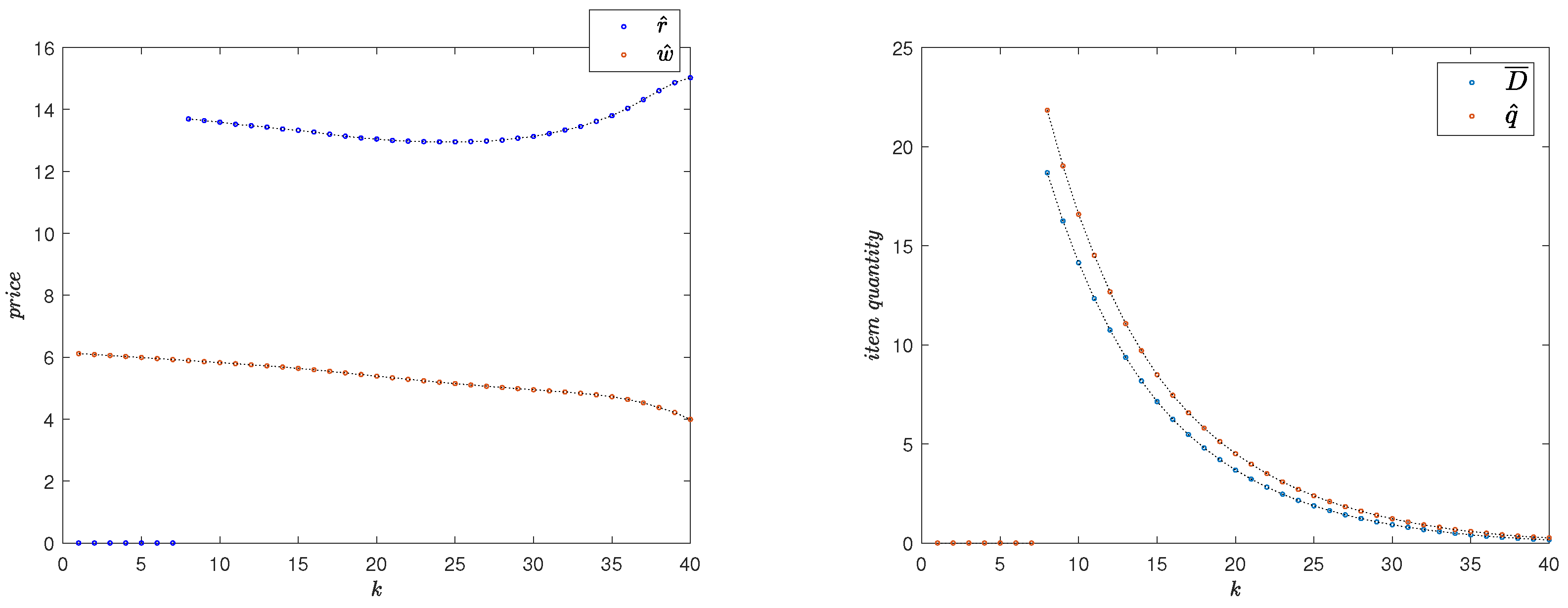
Example 1. In addition to the parameters determined earlier, we set (no discounting), , , , , , and .The optimal pricing variables in each period , as well as the values for (expected demand at k) and (optimal order quantity at k), are shown in Figure 1. In this scenario, for the retailer, the optimal strategy is to increase demand by letting
, then start selling in period 8. Defining the blow-up factor as
, we have
. To obtain increased profits from an initial strategy in which
, it is clearly necessary that
. The total expected profits for the manufacturer and the retailer,
and
, respectively, are found as below.
The relationship between the optimal supplied quantity (
) and expected demand (
) can be interpreted as representative of the level of risk taken by the retailer (i.e., the newsvendor member of the channel). As seen in
Figure 1, in this example, the optimal strategy for the retailer is to over-supply the market with respect to the expected demand
Remark 4. The optimality of an over-supply strategy is not a general phenomenon; as seen in Example 4 (Section 7.3), where the retailer is prescribed to under-supply the market in all periods. In more complicated scenarios, the newsvendor (the downstream channel member) may be prescribed to apply a regime change in its supply strategy with respect to the expected demand. (See a secanrio with both over and under supplying regimes in Example 5, Section 7.4.) The average over-supplying ratio can be measured as For Example 1, this value is calculated as .
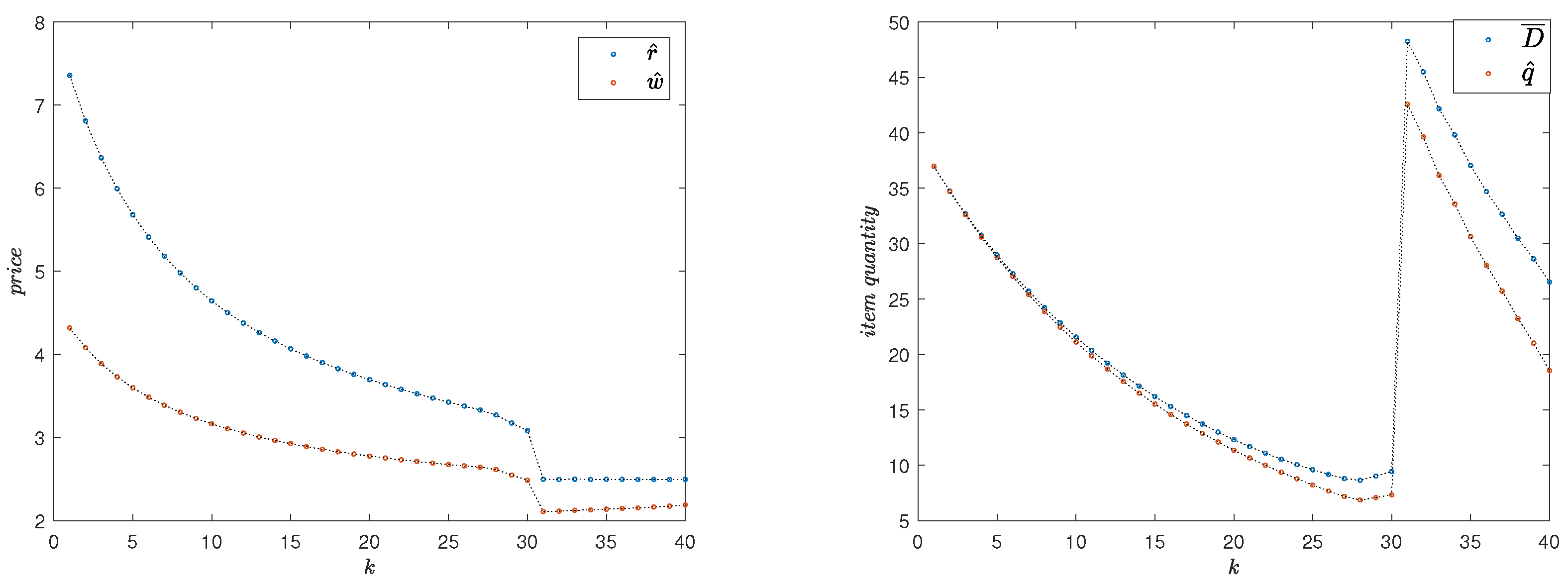
Example 2. In this case, we analyze the previous example subject to discounting: . The rest of the parameters and functional structures are the same as those of Example 1 (Section 1). In this case,
. This blow-up factor is not big enough to justify an initial retail price
. Therefore, sales take place in all periods.
Figure 2 shows the equilibrium prices and corresponding total expected profits for this case. For this case, we find
and
Again, a strategy of over-supplying is prescribed as optimal, with an average over-supply ratio of
.
7.2. Cooperative Agents: Centralized Channel, No Double Marginalization
So far, we have analyzed the equilibria in a Stackelberg framework. However, it is possible for the two parties to merge into a centralized channel. Note that, as outlined in (
5), a Stackelberg equilibrium problem is essentially a bilevel optimization problem wherein the leader optimizes her objective function while being constrained by the optimality of the follower’s solution. Thus, the multi-period single-vendor price-setting newsvendor problem turns into an unconstrained special case of our general model. Such a deviation from the Stackelberg game is implemented by considering the two agents as a single decision-maker, substitution of
in Theorem 1, and optimizing only
with respect to
s.
Example 3. Here, we consider , , , , , , , and . Thus, the integrated channel in Example 3 faces the same market as the one in Example 1.
The results are illustrated in
Figure 3. Due to vertical competition between its members, a decentralized channel suffers from double marginalization leading to its lower performance compared to a centralized supply channel facing the same market. Comparing the results of the centralized channel with its decentralized counterpart analyzed in Example 1, we observe that while the centralized channel charges comparatively lower prices in all periods, its overall expected profit is higher than the sum of expected profits for the two agents in a decentralized channel in the same market. Denoting the total expected profit for the centralized channel by
and the expected profits for the members of the corresponding decentralized channel by
and
(obtained in Example 1), we have:
The centralized channel outperforms its decentralized counterpart while taking a higher risk in its supply quantity; the average over-supply ratio for the integrated channel is 31.74%, compared to 21.9% in Example 1. In addition, relatively lower prices offered by the centralized channel leads to a lower level of demand suppression (compare the expected demands in
Figure 1 and
Figure 3). Thus, unlike the decentralized channel in Example 1, the integrated channel does not need to resort to an early campaign of free distribution of products in order to boost the demand—as observed in
Figure 3, in the case of this integrated channel, sale takes place in all periods.
7.3. Markets with Strategic Customers
The generality of the problem described in
Section 6 and the flexibility of the solution algorithms presented in Theorem 1 and Corollary 1 allows our model to cover diverse sets of market scenarios. The model as a result can be fed with market representation functional much more complex than the ones presented in Examples 1 to 3.
Example 4. Consider a market with two different sets of customer bases. One group, referred to as the strategic customers, postpones their purchase until they see a price lower than their “reservation price". The other group is less sensitive to the offered prices. We assume that the reservation price is known to the channel members. However, the assumption that there exists only one such reservation price among the customers is not necessary and has been adopted for simplification purposes. In general, the customer base can be divided into many factions in the model., , , , , , , As illustrated in
Figure 4, the solution algorithm determines the optimal values for the three decision variables through the periods, and, proposes the optimal timing to begin the
sales season (
). Compare this feature with the prescription of the optimal time to end the free distribution phase in Example 1,
Section 1.
7.4. Positive Network Effects on Demand
Example 5. Demand for certain innovative products is built-up as time goes by through the word-of-mouth effect (see [6,7]). In our model, this network effect, like other externalities is embedded in the demand function via time-dependent functionals. Unlike previous examples, in Example 5, we consider a time-dependent price cap, based on the Bass diffusion model for new-product-adaption: Initially, the price cap is increasing with time, reflecting the customers’ gradually increasing willingness to purchase as time goes by (hence a decreasing sensitivity to prices). Again, we use a simple Cobb–Douglas function for the demand mean functional: . , , , , , , . The shape of the demand results in
Figure 5 are consistent with typical shapes obtained by sales diffusion models. In addition to yielding optimal pricing strategies for the supply channel members at different times, the solution algorithm provides the optimal timing for a change in the supply regime. In the first phase, from period 1 until period 66, the retailer (newsvendor) is better off by under-supplying the market (
); while from period 67, a strategy of over-supplying is found to be optimal.
8. Concluding Remarks
In this paper, we considered a decentralized supply chain composed of a manufacturer and a retailer within a bilevel (Stackelberg) structure. The manufacturer is the (global) leader and the retailer is the follower. The supply chain is to address an uncertain demand within a discretized time horizon. The two agents must strategically solve their respective optimization problems over the entire span of all periods. That is, the final solution algorithm is to give decision variables that are optimizers of the aggregate expected profit over n periods. The ensuing Nash–Stackelberg equilibria, thus, becomes highly interdependent in time. This nestedness has been a challenge in solving Nash–Stackelberg equilibrium problems in a multi-periodic setting within supply chain contracts. Static single-periodic versions of the problem have been solved in the literature. Although mathematically convenient, such reduced static models may turn out to be myopic as they do not cover the after-effects of current pricing on future demand.
In Theorem 1, we introduce a decoupling algorithm that breaks this nestedness and solves the ensuing three interdependent n-dimensional equilibria problems to three sequences of n single-variable equations. In doing so, we prove the existence of a Nash–Stackelberg for a general bilevel optimization problem for the two suppliers in the contract. Next, in the appendices, we show that many supply channel contracts, such as revenue-sharing and buyback contracts indeed produce the same general equilibrium problem structure and hence can be decoupled by our proposed algorithm.
To include strategic customers’ behavior in our model, we implemented a memory-based demand structure. For example, the potential buyers may have become anchored to the past prices and their decision to purchase a product may, to various degrees, be affected by the history of pricing. Such behavioral features are embedded in the model through the introduction of memory functions.
To demonstrate how such Nash–Stackelberg equilibria can be obtained by the recursive algorithm outlined in Theorem 1 and its corollary, we provided numerical solutions to a variety of special cases. Note, however, that our framework is not limited to such special cases. The numerical illustrations raise questions of interest for future research.
In the numerical section, we demonstrated an interesting link to marketing. Under certain conditions, an optimal strategy is to give away products in a pre-sales period. This stimulates demand, and the parties benefit from increased demand in the remaining time periods. Many high-tech products such as mobile phones and computers have a very short lifespan. Our paper, hence, offers a new framework where the optimality of sales strategies for such products can be discussed and analyzed. An example based on the Bass diffusion model for demand is given in
Section 7.4.
The parameters and functional structures that we have used to illustrate the scope of applicability of the solution procedures are merely speculative. To take full advantage of the model, one should try to vary scaling factors and functional forms in a systematic way, for example, through the use of data obtained from empirical studies. Exploring the potential of our modeling approach is a topic for future research.


