
Communication-Enhancing Vagueness

Bureau of Economics, Federal Trade Commission, Washington, DC 20580, USA
Games 2022, 13(4), 49; https://doi.org/10.3390/g13040049
Submission received: 19 April 2022
/
Revised: 4 June 2022
/
Accepted: 13 June 2022
/
Published: 22 June 2022
Abstract
:I experimentally investigate how vague language changes the nature of communication in a biased strategic information transmission game. Counterintuitively, when both precise and imprecise messages can be sent, in aggregate, senders are more accurate, and receivers trust them more than when only precise messages can be sent. I also develop and structurally estimate a model showing that vague messages increase communication between boundedly rational players, especially if some senders are moderately honest. Moderately honest senders avoid stating an outright lie by using vague messages to hedge them. Then, precise messages are more informative because there are fewer precise lies.
JEL Classification:
C91; D03; D831. Introduction
Often, people like to shade the truth by being imprecise. A salesperson might say that he or she receives “few complaints” about an appliance he or she is trying to sell, even if three of the eight customers who bought that model in the past year had complained. A friend might explain his or her absence from a Sunday afternoon gathering he or she did not wish to attend by saying he or she had been “sick all weekend”, even if his or her temperature never went above 99.5 degrees Farenheit.
One characteristic of these vague utterances is that they are explicitly imprecise. This paper experimentally investigates how allowing players the option of sending explicitly imprecise messages instead of precise messages affects strategic information transmission in a standard cheap talk setting, similar to Crawford and Sobel [1].1 Counterintuitively, allowing imprecise messages improves communication—senders on average choose more informative messages, and receivers on average treat the messages as more informative.
An additional contribution of my paper is to explain why communication becomes more effective. In an experimental setting with rational, self-interested players, the kinds of messages available do not matter because in equilibrium, no messages convey any information [1]. However, bounded rationality or honesty might cause players to communicate some information and to treat imprecise messages differently than equivalent precise messages. I find that both characteristics explain subject behavior but that bounded rationality is relatively more important.
In the experiment, the subjects communicate about a state s, which is an integer between 1 and 5. The sender observes s and chooses freely from a menu of English-language messages to send about it. In the base treatment, the menu consists of every message that specifies the state precisely, such as “The state is 3”. The rich language treatment adds three additional messages that specify an interval the state is within, either from 1 to 3, 2 to 4, or 3 to 5 (e.g., “The state is 1, 2, or 3”). After learning the message, the receiver then chooses an action a. The receiver would like to choose , while the sender would like him or her to choose , so they play a partial common interest game [4].
With either message space, with rational payoff-maximizing players, no Bayesian Nash equilibrium equilibrium exists in which m conveys any information about s, and as a result, a choices are independent of m. However, subjects in both treatments send messages that convey more information than optimal and are more trusting of messages than they should be.
This “overcommunication” finding is typical (e.g., Cai and Wang [5] or Duffy et al. [6]; see Blume et al. [7] for a general overview). The prior experimental literature has alternately explained excess communication through preferences for truth-telling [2,8,9,10,11,12,13,14] or bounded rationality [5,15,16,17].2
Comparing their relative importance can be difficult, because from a money-maximizing perspective, honest behavior will seem unsophisticated. To compare them, I develop a model which teases out distinct implications of honesty and bounded rationality across my treatments. My model adapts the one-parameter Poisson cognitive hierarchy model in Camerer et al. [18] to cheap talk and combines it with some players receiving a non-pecuniary benefit from truth-telling.
In structural non-equilibrium models such as cognitive hierarchy or level-k models, players have a (typically incorrect) belief about how other players are acting and optimize given their beliefs.3 Players vary in the sophistication of their beliefs. Level 0 () players act non-strategically—in this context, by either being truthful or by being completely credulous—while players are defined inductively and believe all players are of lower levels. Due to the upward bias, for instance, senders exaggerate s by choosing . If the receivers think a few senders are but most are , they discount messages by choosing , but they think are truthful and do not discount them. Following Camerer et al. [18], I assume that the players’ levels have the Poisson distribution. Many qualitative aspects of my subjects’ behavior match this sort of reasoning.
Players vary in their honesty types in addition to their cognitive types. A player’s honesty type indicates how strong a preference for truth-telling he or she has and can be thought of as reduced-form behavior combining a variety of factors. Some subjects behave as if they dislike sending literal false messages (i.e., “lies”, following Sobel [24]’s definition). This form of honesty is the most straightforward explanation for why senders’ message choices would be qualitatively different in the two treatments.
I am agnostic about the underlying reason my subjects behave in this way, though. Recent experiments show that in non-strategic settings, subjects seem to be motivated by honesty preferences that combine a direct cost of lying and a cost for being identified as a liar [13,14]. The dislike of sending literal false messages embodied in my model’s honesty types could stem from either of these explanations.
Players who care little about being honest, players who care moderately about being honest, and players who care strongly about being honest all should exhibit distinct behaviors in my experiment. The rich message treatment enables players to truthfully exaggerate, such as by sending the message “The state is 1, 2, or 3” when the state is really 1. All players believe that precise lies are more effective deceptions than truthful exaggerations, especially when the state is high. Like weakly honest players, moderately honest players in the base treatment should not send honest messages because the monetary loss from forgoing precise lies is too high. However, moderately honest players should engage extensively in truthful exaggeration in rich treatment. Finally, strongly honest players should be honest even when truthful exaggerations are not available in the base treatment.
Subject behavior across the treatments was more consistent with moderate honesty than strong honesty. Overall, 45% of the messages sent in the rich treatment were imprecise, and 57% of the imprecise messages were truthful. On the other hand, in the base treatment , only 15% of the messages were truthful.
I then estimate a simple structural model using maximum likelihood with two parameters of interest: , the average cognitive level of the subjects, and , the fraction (and subjects’ beliefs about the fraction) of moderately honest players. Most of the subjects in my experiment employed one or two levels of exaggeration or discounting (i.e., rounds of best-response reasoning). About a quarter of the subjects showed moderate preferences for honesty.
Despite the presence of honest players, when these estimates are used to calibrate my model, they imply that honesty plays a limited role in explaining why communication increases in rich language treatment. Just as important as honesty are two other factors. First, the model implies that precise messages are more informative in rich message treatment independent of honesty. In that treatment, senders of all honesty types often choose imprecise messages instead of precise ones if they observe a low state. Removing the most misleading lies from the pool of precise messages improves the accuracy of the precise messages. Second, I estimate that players are somewhat less sophisticated in their reasoning in the rich language treatment. The reduction in the average levels of reasoning seems likely to be driven by the increased complexity of strategic calculations in the rich language treatment. In the calibrated model, this reduction in sophistication manifests largely through increased receiver trust in the messages.
Several groups of experimental papers are closely related to this paper. My experimental setup in the base treatment mirrors Cai and Wang [5] and Wang, Spezio, and Camerer [15]. They explained the overcommunication in their experiments using level-k but did not allow preferences for truth-telling in their models or investigate the impact of vagueness.4, those choices caused the computer to randomize between states in an interval. The receivers always received a point message and were not informed that it was randomly chosen.
A second pair of experimental papers investigated how senders use vague or evasive language in simpler two-state strategic information transmission settings [25,26]. These found that deception through evasive messages such as feigning ignorance is less psychologically costly than deception through direct lies.
A third set of papers investigated information unraveling in voluntary disclosure games, in which the subjects were only able to send truthful messages. Benndorf et al. [27] elicited a distribution of level-k types in a disclosure game, finding substantial numbers of , , and players. Jin et al. [28] and Deversi et al. [29] both used state spaces and payoff functions very similar to those in my experiment. Jin et al. [28] found that senders disclose favorable information but withhold less favorable information, and receivers are insufficiently skeptical when information is not disclosed. Deversi et al. [29] examined what occurs when senders can choose imprecise disclosures. They found that vagueness is profitably exploited by senders to take advantage of naive receivers, and information transmission is higher in their precise-only treatment. Hence, interestingly, my result that vagueness improves communication is reversed for disclosure games (see also Li and Schipper [30] and Hagenbach and Perez-Richet [31]). Unusually, Li and Schipper [30] found that the subjects exhibited relatively high levels of sophistication in a disclosure game with imprecise messages.
Many other papers investigate the role of vague language in other forms of cheap talk games, including asymmetric coordination games with private information [32], leader-follower public goods games [33], delegation games [34], cheating games [35], three-player common interest context-dependent communication games [36], and real-world communication about intentions on a TV game show [37]. Like this paper, these papers found that subjects, given the choice, prefer imprecise messages to outright lies, and followers are too trusting of these messages. In some, vagueness is beneficial either because it can mask incentives that, if known, would make an attractive equilibrium strategically unsustainable [32,33], because it makes information more credible [34], or because it enables more efficient communication of context-dependent information [36].
Relative to these sets of papers, my contribution is to show that vagueness can have positive effects on communication in strategic information transmission contexts and offer an explanation for why it has positive effects.5
2. Experimental Design
My experimental design builds on those of Cai and Wang [5] and Wang, Spezio, and Camerer [15], which are discrete versions of the Crawford and Sobel [1] cheap talk game. In each period, subjects were paired up, with one member of each pair being the sender and one being the receiver. A state of the world was then randomly determined for each pair. Each state was equally likely. The sender then learned s and chose to send to the receiver. The message space M—the set of possible messages—varied across treatments. Finally, the receiver learned m and chose .
The sender and receiver payoffs (in experimental units) were
The subjects were presented with payoff tables similar in format to Table 1 below, although with neutral labels instead of “sender”, “receiver”, “action”, and “state”.
There were three treatments. In the base treatment, the sender could send only precise messages of the form “s is x” (i.e., the message space was ). In the rich language treatment, the sender could choose to send either precise messages or imprecise messages. Imprecise messages specified an interval of three numbers that s could be within, such as “s is 2, 3, or 4”, so the message space was .
Finally in a third treatment (the noise treatment), the sender observed s imperfectly and could send precise messages or imprecise messages (). Instead of observing s, the sender observed where was equally likely to be any element of and s was equally likely to be any element of . In practice, choices in the noise and rich treatments were indistinguishable, so I added the noise data to the rich data, setting for noise observations.6
Three principles guided the construction of . First, having only a few additional messages made the choices easier for the subjects and simpler to analyze subsequently. Second, contiguous messages with intermediate precision of meaning suggest a natural interpretation of low, medium, and high. Third, the precise messages were uniformly distributed over the state space, and I chose to maintain that property for the imprecise messages.
Instructions for each treatment were handed out and read aloud at the start of that treatment. (Appendix B contains the experimental instructions.) The experiment was conducted using z-Tree software [42] at Clemson University in the fall of 2011. There were 42 subjects, 18 (42%) of whom were female. 24 (57%) subjects were first- or second-year college students, while 18 (43%) were third-year, fourth-year, or graduate students. The subjects were mostly College of Business and Behavioral Sciences undergraduates: 32 (76%) had majors in the business school, 4 (10%) had humanities majors, and 6 (14%) had science or engineering majors.
The subjects alternated roles and were randomly rematched each period in order to avoid repeated game effects. All subjects participated in all treatments, and the order of the treatments was randomized for each session.7 In total, there were 268 rounds of the base treatment, 204 rounds of the vague treatment, and 220 rounds of the noise treatment (there were 4–6 rounds for each treatment). Note that a round yields one message choice observation and one action choice observation. Each experimental unit was worth USD 0.01. The average earnings were around USD 24, which included a USD 6 payment for showing up.
3. Results
Table 2 shows the state from which each message was sent, on average, along with the frequency of each message. Over half of messages in the base treatment were , which led to that message not being especially informative, with . Generally, the lower the message, the less likely it was to be chosen, and the stronger the signal it provided that s was low. In the base treatment, and conveyed different information than the other messages: the distribution of s, conditioned on , was significantly differerent at the 10% level from that for (two-tailed Mann–Whitney U test ), and the distribution for was significantly different from at the 1% level (MW ).
The rich treatment produces three related effects. First, higher messages become more accurate. For messages above , a precise message is a stronger signal that s is higher in the rich treatment than in the base treatment, while is 57% closer to its literal meaning (rich language versus base , MW ), and is 17% closer (rich language versus base , MW ). is also 43% closer to an expected than is the base treament (rich language versus base , MW ).
Second, almost half of the messages (45%) sent become imprecise, and imprecise messages are twice as likely as precise . Imprecise messages are less likely to be sent from but otherwise are employed about half the time in every state.8 Such a high fraction of imprecise messages is inconsistent with many explanations of my subjects’ behavior. For example, the analysis in Section 4 found that most variants of the level-k models without honesty could predict that, at most, 20% of the messages would be imprecise, and those would predominantly be sent from and .
Third, the messages overall become less exaggerated. While 51% of the base treatment messages were , only 34% of the rich treatment messages were the highest possible. The difference was statistically significant (Fisher’s exact test ). The fraction of messages with an expected value of 4 (i.e., or ) doubled from 18% to 36% in the rich treatment (Fisher’s ). None of the other message frequencies were significantly different between the treatments when comparing all messages of the same expected value, except for , which went from 6% to 2% of the messages (Fisher’s ).
The receivers correctly treated the messages as informative, although many systematically misinterpreted them. Table 3 shows both the average and optimal action choice for each message. The optimal action choice is the highest-payoff action choice given the true distribution of messages. On average, the chosen a values were too high for both treatments but showed the “correct” comparative static of lower actions when receiving a lower message.
When comparing the responses in the rich treatment to the base treatment, the typical actions did not change much. With the exception of the responses to , for which increased from 3.47 to 3.79 (MW ), the hypothesis that the receivers’ responses to precise messages were the same across treatments could not be rejected. In addition, the responses to were systematically higher than the responses to the precise treatment (MW ). These patterns were consistent with the level-k behavior, as Section 4 explains. Figure 1 shows the full distribution of relative frequencies for each message in the precise and rich treatments. For and , the most likely state from which the message was sent was the corresponding state or , while for , with the exception of precise in the rich treatment, the true state was never the most likely. Consistent with the initial level-k reasoning that sends , messages or were most likely to have been sent from in both treatments. In the base treatment, exaggerating by two units is common with and as well, but in the rich treatment, two-unit exaggerations were less typical.
Next, Figure 2 shows the frequency of each action for every message sent () in the base and rich treatments. Consistent with the level-k predictions, there was widespread discounting of messages by two units, such as choosing in response to . The discounting was less pronounced for , imprecise messages, and in the rich language treatment.
Figure 1 and Figure 2 also show that the m and a choices were quite noisy in both treatments, with the exception of in the base treatment, for any s, and generally for all s. This noisiness means that usually, the receivers would maximize utility by adjusting their action choices inward toward (as in Table 3).
While the number of subjects was too low to perform a detailed analysis of how different demographic characteristics affected communication choices, I did find a few differences in how the subjects behaved based on gender or college class year. The female subjects were less trusting of messages in the precise treatment than the male subjects, with a mean distance between the message they received and the action chosen of 1.39 versus 1.18 for the male subjects (MW ). Gender differences were not statistically significant at the 10% level in the vague treatment or for the messages sent. I also found that the first- and second-year college students sent much more accurate messages in the rich language treatment than the third-year, fourth-year, and graduate students. The average distance between the state and the message sent was 1.08 compared with 1.39 (MW ). Again, however, there were no other statistically significant differences in behavior either in the precise treatment or with the action choices.
Finally, there was no evidence that the players’ strategies changed during the sessions on aggregate. In particular, the fraction of imprecise messages was roughly constant in the early and late rounds, as was the share of truthful messages and the degree of discounting by receivers, ruling out sizeable learning effects.
4. Model
This section derives predictions about the subjects’ behavior using a cognitive hierarchy model, to which I add preferences for honesty. Cognitive hierarchy and level-k models are structural nonequilibrium models of how players reason strategically. There is a hierarchy of discrete cognitive types, each with gradually more sophisticated beliefs about other players’ behavior. Because higher types use more iterations of best-response reasoning, senders of higher types exaggerate more and more due to their upward bias, while receivers of higher types discount the messages more and more. My model extends the applications of level-k from Crawford [21] and Cai and Wang [5] to cheap talk by allowing heterogenous preferences for truth-telling on the part of the senders. A secondary difference is that I assume that players best respond to a combination of behaviors of types lower than k.9
The model has two purposes. First, it illustrates the broad differences in behavior one should expect between my treatments if the subjects are boundedly rational and some are honest. Second, the next section estimates the model structurally, taking into account that it is not likely that any subject perfectly complies with the predicted behavior of any type.
4.1. Definitions and Assumptions
Formally, players differ in their cognitive type, honesty level, and sender or receiver role. A player’s cognitive type determines his or her beliefs about how players in the other role behave. A level-k sender () has beliefs about the conditional probabilities induced by receiver behavior, and a level-k receiver () has beliefs about the conditional probabilities that he or she faces.
A player’s honesty type affects his or her relative utilities from sending dishonest or honest messages. All messages that are non-false according to their literal meaning are honest (i.e., m is honest if either or ) and are dishonest otherwise. I discuss this assumption further in Section 4.3. An honesty type h acts as if sending a literally true message is worth giving up h cents:
A receiver’s utility function is not affected by his or her honesty type. I assume that there is a finite set of honesty types, with every . The vector denotes the distribution of honest types, and I write to indicate the fraction of players with honesty type h. H and are common knowledge.
Level 0 cognitive types are non-strategic and primarily serve as conjectures about behavior by players. messages are truthful, and messages are credulous.10 Strategic behavior is then defined inductively as responding optimally to beliefs about the other role’s behavior based on behavior.11 A level- sender chooses for each state a (possibly) mixed strategy over messages as a best response to that type’s beliefs about receiver behavior. Likewise, a level- receiver chooses , which is a best response to his or her beliefs about the sender’s behavior.
Definition 1.
A type player sends every available honest message with equal probability. A type player chooses action if m is precise and if .
In the Poisson cognitive hierarchy model of Camerer, Ho, and Chong [18], the frequency of level-k behavior follows the Poisson distribution, and the level-k beliefs about the frequencies of type players are formed by normalizing to sum up to one:
By definition, is the mean cognitive level in the population as well as the variance of the cognitive levels in the population.
Definition 2.
For , a type player with honesty h has beliefs and chooses that follow
and a type player has beliefs and chooses that follow
where is calculated via Bayes’ rule.
To operationalize Equation (2), I assume that for cases in which the senders are indifferent between multiple m, they randomize uniformly over their best messages.
It is helpful to think of honesty as falling into three levels: “weak” (), “moderate” (), and “strong” (). These categories are based on the opportunity cost of being honest in different situations (i.e, the loss in pecuniary payoff for sending an or message versus the best non-honest message). In the base treatment, and believe that they can achieve with or remain honest and achieve at a loss of .12 On the other hand, in the rich treatment, low-level senders perceive the opportunity cost of honesty to be either 25 or 32 for sending an imprecise message which is a truthful exaggeration. For instance, for , when , has an opportunity cost of .
In presenting the model’s predictions but not estimating the model, I restrict attention to a set of parameters that encompasses most reasonable distributions of the types and for which the strategies of each type of player are largely constant. The restriction also limits the number of special cases that need to be described. Let the constant . c is proportional to the difference in payoff cost to the sender or receiver having an action choice 2 away from the player’s bliss point instead of 1 (i.e., a loss of instead of a loss of 25). Let be the share of players with honesty .13
Definition 3.
A standard type distribution of players has frequencies of cognitive and honesty types that are distributed with
This range is consistent with the estimates from other papers and with my preferred estimates. The restriction on asserts that roughly between 15% and 50% of my subjects are at least moderately honest which, again, is consistent with my estimates.
4.2. Predictions
Particular patterns of behavior for a role are usually common to pairs of cognitive types. best responds to , implying . That in turn implies and both effectively use one round of best responses, since both types believe all receivers are credulous. If is high enough that the players believe the players are uncommon, the and receivers act similarly as well. ’s best respond to a fraction of truthful messages and a fraction of single-level exaggerated messages, which are quite close to ’s beliefs for reasonable choices. Likewise, the and senders typically engage in two rounds of non-trival best-response reasoning, and so on.
Propositions 1–4, summarized in Table 4, Table 5 and Table 6, characterize the behavior of senders and receivers drawn from a standard type distribution in my experiment. See Appendix A for proofs.
Proposition 1.
If the players have a standard type distribution, and no players are strongly honest, then the following is true for weakly honest senders and all receivers in the base treatment:
- (i)
- and exaggerate one level if possible ();
- (ii)
- and discount and by two units (), by one unit (), and or by zero units ();
- (iii)
- and higher-level senders send the highest message except possibly when or (in which case and ); and
- (iv)
- and higher-level receivers discount one unit (), by zero or one unit ( or ), and all other by two units (.
Moderately honest senders make identical choices to weakly honest senders, except that and choose .
Table 4 summarizes the types’ predicted behaviors in the base treatment. Proposition 1 predicts that messages should be relatively rare, relatively truthful, and the receivers should trust them more. The truthfulness of the low messages does not stem from honesty. For , many messages are exaggerations by two units, and the receivers discount them, often by two units. Finally, most of the messages are .
In the base treatment, for players with , and would send . Then, if was low, and higher would discount it by the same amount as in Proposition 1 or by a smaller amount if was higher. That discounting makes honesty more costly to and higher, so unless there is a significant share of players with h significantly higher than 57, the behavior for the higher types becomes similar to that in Proposition 1. Thus, strong honesty would cause a sizeable share of honest messages and trusting action choices for as well as for for .
In the rich treatment, randomize between truthful precise and truthful imprecise messages. This leads to and with choosing imprecise messages , which exaggerate the state in a truthful way. In addition, weakly honest and send imprecise m deceptively () half the time in states and .
Both honest and non-honest level- senders employ imprecise messages, but exactly how they do so on depends whether they believe imprecise messages will be treated skeptically or credulously. Weakly honest level- senders often choose to masquerade as honest or naive types by sending imprecise messages but only when the state is low (). For example, for these senders, the message is an attractive deception in because they believe there is a good chance that , regardless of exactly how low-level senders use imprecise m.
Whether there is truthful exaggeration by moderately honest level- senders depends on what they believe receivers believe. If relatively few of the low-level imprecise messages are deceptive—which occurs either if is low enough or is high enough—then the and receivers are fairly trusting of imprecise messages and choose when they usually choose . Because of these a choices, moderately honest level- senders also send imprecise messages in states . In contrast, if a critical mass of non-deceptive messages is not available, low-level receivers are less trusting of imprecise messages, and these senders make use of imprecise messages in the same way as weakly honest senders because honesty is too costly.
Therefore, if imprecise messages are sent frequently from and , and and are trusted more than the corresponding precise messages, it cannot be the case that is high and is low. In order to generate the pattern of imprecise messages observed in the data, there must be higher-honesty senders sending imprecise messages from and as well.
Table 5 and Table 6 organize the predictions of the following propositions describing behavior in the rich treatment.
Proposition 2.
If players have a standard type distribution, then weakly honest players in the rich treatment choose identical strategies to those in Proposition 1 above, except for the following:
- (i)
- and in states and send with probability ;
- (ii)
- or higher-level senders in state send or ;
- (iii)
- and senders in state may send .
Weakly honest senders do send imprecise messages but only in low states (). In contrast, senders who care more about honesty tend to send imprecise messages in every state except .
Proposition 3.
If players have a standard type distribution, then moderately or strongly honest senders () in the rich treatment behave as in Proposition 2 above, except for the following:
- (i)
- and truthfully exaggerate in and send and with equal probability;
- (ii)
- truthfully exaggerate in , except possibly in ;
- (iii)
- and truthfully exaggerate in and may also truthfully exaggerate in , , and .
While the senders change their behavior in the rich message treatment, the receivers’ predicted responses to precise messages do not change. However, receivers generally trust imprecise messages more than precise ones (e.g., sophisticated receivers choose , while they would choose ).
Proposition 4.
If players have a standard type distribution, then in the rich treatment, receivers behave as in Proposition 1 above, except for the following:
- (i)
- and do not discount imprecise messages ();
- (ii)
- and higher discount imprecise messages by one unit (), except possibly discounting by two units ();
- (iii)
- and higher do not discount precise ().
4.3. Model Discussion
Propositions 1–4 provide an explanation for why there is more communication in the rich treatment. Under a standard type distribution and, indeed, under most other type distributions, many player types who would send from in the base treatment instead send a different message in the rich treatment but continue to send from at the same rate. These messages therefore become more accurate in the rich treatment. Furthermore, the imprecise messages sent with are more accurate than the corresponding messages that would have been sent with . For instance, and higher send some from and , whereas and are usually sent from and with . The receivers do not change their responses much, but because they discount the common and the least, on average, they are more trusting of the messages they receive.
The model’s predictions match several patterns in the data. First, the model predicts that the sender’s behavior will be relatively more responsive than the receiver’s behavior to the rich message treatment. Precise messages and are predicted to become more accurate, since they are less likely to be sent from (Propositions 2 and 3). For many parameter values, the messages sent from are also predicted to often be imprecise. The receivers, on the other hand, are predicted to not change how they treat precise messages across the treatments (Proposition 4 (iii)) and to be somewhat more trusting of imprecise messages and than corresponding precise messages (Proposition 4 (i) and (ii)). Note that all of the comparative statics implicitly hold constant. However, is more complex, so might fall as well.
The form of honesty preferences in the model generates (1) receivers treating systematically differently than and (2) half of messages sent in the rich treatment being imprecise messages. Many alternative forms of honesty preference do not predict either. For instance, theories in which the senders care about the payoff disappointment experienced by the receiver, because and interpret and in the same way, would predict no systematic difference in how the senders used those messages. Likewise, there would be no systematic differences if the senders cared only about the de facto level of deception (i.e., , where E is the receivers’ expectation) instead of caring about deviating from the literal meaning of a message.
A major difference between the predicted and observed behavior is that the model predicts more skepticism about precise than is observed. senders and higher are predicted to play . In part for this reason, I introduce noisy choice when estimating the model parameters.14
5. Structural Estimates
In this section, I estimate the parameters of my model. Many papers have structurally estimated level-k models before (e.g., Crawford and Iriberri [43]), but to my knowledge, none have jointly estimated varying cognition levels and varying preferences. One goal for these estimates is to conduct a “horse race” between honesty and bounded rationality, but by using these estimates, I can also answer additional questions, such as how the different message spaces affect communication per se.
I assume that the subjects choose a or m, influenced by logistic errors of precision and independent across rounds and treatments. These errors capture that level-k reasoning is subject to error and unobserved utility shocks may occur, as well as any other sources of error. Hence, a level-k sender or receiver chooses each m or a with a probability
where is a level-k sender’s beliefs, is a level-k receiver’s beliefs, T is the treatment, and h is a sender’s honesty type. measures the noisiness of player choices. As , each choice becomes equally likely, while as , players best respond exactly according to their beliefs. For all , the players exactly follow the strategies specified in Definition 1.
For my preferred estimates, I restrict the honest types to either have (the “not honest” type) or (the “moderately honest” type), because it is hard to precisely identify the frequencies of more than two honesty types. I motivate this choice and discuss exactly what conclusions can be drawn about the distribution of honesty after presenting my base estimates.
Given a treatment T, in which subject i made action choices and message , the probability of i’s observed choices for a given parameterization is
For a set of subjects N, the log likehihood of their observed behavior in a set of treatments is
I estimate the parameters by maximizing and then derive confidence intervals through non-parametric bootstrapping.15
Column 1 of Table 7 reports the parameter estimates for my entire dataset. The estimated mean steps of reasoning was higher than that typical in the literature. However, given the definitions of behavior for each role, the effective amounts of sophistication were similar. These estimates imply that 32% of the senders engaged in one iteration of strategic reasoning and 40% of the senders engaged in two iterations, while 16% of the receivers did not reason strategically (they were credulous). Additionally, 42% of the receivers engaged in one iteration of strategic reasoning, and 42% engaged in two or more iterations.16 Cai and Wang [5] and Wang et al. [15] found comparable results. About 27% of the subjects had or were believed to have . Finally, the choices were noisy. For example, the estimated precision implies that moderately honest types sent 10–20 percentage points fewer imprecise messages than they would without noise and that the weakly honest types sent 20 percentage points more imprecise messages than they would without noise.
The next columns report my model, estimated separately using the data from the rich treatment only (column 2) and the base treatment only (column 3). Reasoning was almost one level less sophisticated in the rich treatment than the base treatment, probably reflecting the greater difficulty of mental calculations involving . The choices were approximately as noisy. Not surprisingly, the confidence interval for in the base treatment was wide— could not easily be identified using choices over —but the estimates in model 3 were similar to those in the combined model (model 1).
The final two columns in Table 7 report the model estimates using only the sender choice data (column 4) or receiver choice data (column 5). That the estimates were even lower in model 5 than model 4 support the somewhat strange implication of my cognitive hierarchy model that receivers are less strategically sophisticated than senders (i.e., only senders are naive, but and both act naively). If this assumption were inaccurate, one would expect the estimate in model 5 to be higher than the estimate in model 4. It seems likely that the strategic reasoning that receivers must perform is more difficult than the strategic reasoning that senders must perform.17
The model pair of 2 and 3 and the pair of models 4 and 5 can be thought of as alternate models that relax one of the assumptions of my level-k model. The combination of models 2 and 3 allows and to vary by treatment instead of forcing strategic sophistication to be constant. This treatment-varying specification (models 2 and 3) nests model 1 as a special case, and a likelihood ratio test comparing the null hypothesis (model 1) to the alternate (models 2 and 3) rejects the null at the 0.05 significance level (, ). This is evidence of the systematic differences in the level and noisiness of reasoning between the two treatments.18 A similar likelihood ratio test comparing the null hypothesis (model 1) to the alternate model with role-varying behavior (models 4 and 5) failed to reject the null hypothesis (). Comparisons using the Bayesian Information Criterion, which assigns more importance to model parsimony, support the role- and treatment-invariant model (model 1) () over either the treatment-varying or role-varying model ( and , respectively, for the combined models).
5.1. Honesty
The distribution of honesty was identified in two ways. First, the strength of the players’ preferences for honesty was identified through the qualitatively different behavior of weakly, moderately, and strongly honest senders. For instance, senders with moderate honesty should reliably and truthfully exaggerate in the rich treatment but not reliably send truthful messages in the precise treatment. Second, the fraction of players of a given honesty type (i.e., for a given h) was identified through the magnitudes of honest behavior and through their indirect effect on how receivers and non-honest senders behave. Section 4 described some of the identifying differences in greater detail. For instance, if is low and is high, the receivers should be relatively skeptical of imprecise m, and the senders should send relatively few imprecise m from states and . Figure 3 shows the distribution of from the bootstrap for my preferred model. Most estimates are between and , although there is an almost invisible left tail for the lower estimates.
Unfortunately, the log-likelihood function was relatively flat with respect to the strength of honesty preferences within each of the h intervals of not honest, moderately honest, and strongly honest. Figure 4 shows the maximum log-likelihoods from two-honesty-type models, where one type does not care about honesty and the other type is h. Intuitively, for low honesty, was estimated entirely from how it interacted with utility shocks in the message and action choice (Equations (5) and (6)), while within each of the other h intervals, the variation in behavior was small, so pinning down h precisely was difficult. The may have also been flat with respect to h, because honesty has limited importance in my context. These problems also made it infeasible to estimate the frequencies of the honesty types in a richer model that contained two honest types . Because the behavior is similar for any moderately or strongly honest type, the parameters and are colinear and cannot be estimated precisely.
Due to these difficulties, my approach is to assume that people are either fully self-interested or have a single degree of honesty h. For each h value, Figure 5 shows the fraction of players estimated to be honest at this level and the 95% BCa confidence intervals. For any moderate honesty level, at least around 15% of players can be classified as honest with 95% confidence. I focus on because the log-likelihood achieves its maximum at that value (see Figure 4).
Despite the underlying identification problems, there is evidence that a substantial minority of subjects had at least moderate preferences for truth-telling and believed that other subjects did as well. While I am could not estimate the exact distribution of honesty in my subjects, I am able to show both that it was not extremely weak (all subjects having ) and that only a minority of the subjects had moderate or strong honesty preferences.
5.2. Why Vague Language Matters
Counterfactual comparisons using the structural model can also answer the question of why vague language improves communication. Communication might increase in the rich treatment either because it affects subjects’ decision processes in terms of reducing their sophistication or increasing choice noisiness, because the change in the message space opens up additional ways to communicate, which improves communication overall, or because honesty increases sender accuracy or receiver trust more under the more complex message space. To gauge these explanations’ relative importance, I hold some factors as fixed and evaluate how the predicted communication change as a single factor changed. For example, if strategic sophistication is fixed at the base treatment levels, and all players are assumed to be weakly honest, the predicted improvement in communication from adding imprecise messages to the message space is a measure of how important the change in the message space is according to my model.
To measure communication, I calculate the predicted mean distance between messages and states to measure how informative the messages are and the predicted mean distance between actions and messages to measure how trusting the action choices are.19 Given a set of a parameters , , and and a message space M, the mean distance between the messages and actions is the distance between each combination weighted by the predicted probability of observing that combination:
where is the predicted probability that message m is sent (obtained from Equation (5)) and is the predicted conditional probability (obtained from Equation (6)). is defined similarly but with weights instead of .
Table 8 reports these measures for every combination of behavioral parameters and each message space. The rich language parameters are model 2’s: the MLE parameter estimated using only rich language treatment data. Rich honesty sets , while rich rationality sets and . The base treatment parameters are those of model 3. Base honesty sets , while base rationality sets and .
The first two rows compare the average distances in the base treatment data to the predicted average distances from calibrating the model with the parameter estimates from MLE using the base treatment data. The mean distance in the data was 1.52 in comparison with the predicted of 1.46, while for the receiver mean in the data, it was 1.30 in comparison with the predicted distance of 1.28. The calibrated model closely matches senders’ average exaggeration and receivers’ average skepticism.
The last two rows provide the same comparison for the rich language treatment. For the senders, the mean distance in the data was 1.22, while the model predicts a mean distance of 1.16. For the receivers, the mean distance was 0.98, while the model predicts a mean distance of 1.05.
The intermediate rows use alternative model calibrations to show which factors are important in the model for explaining the observed increases in communication. The three rows after the base treatment model each switch one factor from its value in the base treatment model to its value in the rich language treatment model. The next three rows then switch two factors from their values in the base treatment model to their values in the rich language treatment model. Factors that cause larger reductions in sender bias or receiver skepticism are more important in the model for explaining the increase in communication. To the extent that the model accurately captures aggregate behavior, these factors are likewise more important for explaining what caused the changes in subject behavior across the treatments.
For senders, the most important factor appeared to be the message space. Switching to a rich message space in the model but holding the behavioral parameters fixed at the base model values causes the mean to fall to 1.30 from 1.46, a larger effect than for switching any other single factor. Similarly, when two factors were switched, the cases that come closest to matching the predicted mean of 1.16 in the rich language treatment are the cases in which the message space and one behavioral parameter are switched to their values in the rich language model.
In my model and in my reduced form results, a rich message space improves sender accuracy because many senders shift from and to imprecise messages, making the high-m precise messages more accurate. This shift to imprecise messages, while most pronounced in the model for honest senders, occurred with all senders in low states.
For receivers, the most important factor appears to be the bounded rationality parameters of the mean steps of thinking and choice precision . Switching to the rich language model and parameter values but holding the message space and share of moderately honest players fixed at the base model values causes the predicted to fall to 1.08 from 1.28, a larger effect than for switching any other single factor. When two factors are switched, the cases that comes closest to matching the predicted of 1.05 in the rich language treatment are the cases in which the rationality parameters and one other parameter are switched to their values in the rich language model.
The increased cognitive complexity of strategic thinking in the rich message treatment made subjects worse at strategic reasoning, which manifests in the model estimates as a reduction in . Reducing makes the receivers more trusting, because the lower-level receivers engage in fewer rounds of iterated reasoning, which tends to mechanically increase receiver skepticism.
Interestingly, for the receivers, the model predicts that switching to the rich message space would cause a slight increase in the average receiver skepticism if honesty were not present. Switching to a rich message space in the model but holding the behavioral parameters fixed at the base model values causes the predicted to rise from 1.28 to 1.33, and likewise, switching to a rich message space in the model with the rich language model’s and and base model’s causes the predicted to rise from 1.08 to 1.14.
In summary, three factors explain the increase in communication produced by the rich treatment. The richer message space made the senders more accurate, while the increased difficulty of reasoning for made the receivers more trusting. The presence of honesty also reduced receiver skepticism when they were interpreting the messages.
6. Conclusions
It is natural to think that when people make use of less precise language, communication will become less effective if they do so. Surprisingly, in a standard biased information transmission setting with high sender bias, when the subjects could choose between more or less precise messages, the distribution of messages conveyed more information, and the receivers were more trusting than when the subjects could only send precise messages.
Communication was improved because the senders changed the least accurate messages they sent to imprecise ones if they were available, making both the precise messages and imprecise messages more informative as a result. It is also improved because the receivers were somewhat more trusting due to both the increased cognitive difficulty of strategic thinking and the greater prevalence of honest message choices. A larger share of honest messages was sent due to the lower opportunity costs of honesty when honest imprecise messages could be chosen.
Strategic information transmission games are a natural setting in which to expect strategic miscalculations to be important, as the incentives for exaggeration are especially salient. At the same time, what norms of honesty should operate are unclear. Honesty did play a small role in explaining why communication increases when the message space was enriched by adding explicitly imprecise messages. In a population with honesty, the receivers’ trust in the messages increased slightly more with a rich message space than it would otherwise. Nonetheless, most of the improvement in communication seemed to be due to the change in the message space or bounded rationality combined with the increased complexity of the message space. In other strategically simpler settings or those in which honesty is more salient, honesty might be relatively more important.
Funding
This research received no external funding.
Institutional Review Board Statement
The study was conducted in accordance with the Declaration of Helsinki, and approved by the Institutional Review Board of Clemson University (IRB#2011-110, approval date 30 March 2011).
Informed Consent Statement
Informed consent was obtained from all subjects involved in the study.
Data Availability Statement
Publicly available datasets were analyzed in this study. This data can be found here: https://sites.google.com/site/dhwood/.
Acknowledgments
The views expressed in this paper are my own and do not necessarily reflect those of the Federal Trade Commission or any individual Commissioner. I thank Dave Schmidt, Ernest Lai, Heinrich Nax, Patrick Warren, Tom Lam, John Smith, Joseph Tao-Yi Wang, Ryan Kendall, Karl Schlag, Gary Charness, Joel Sobel, Vince Crawford, and seminar audiences at Clemson, the 2015 ICES Conference on Behavioral and Experimental Economics, the ESA 2011 World Conference, and the 2015 Econometric Society World Congress for helpful comments. I also thank the two anoymous referees for their very helpful suggestions.
Conflicts of Interest
The author declares no conflict of interest.
Appendix A. Proofs
Appendix A.1. Proof of Proposition 1
Weakly honest and play because they expect , and indeed, senders play . senders believe or comes from and as such choose . The message could come from in or in , and thus
Therefore, if
which holds for a standard distribution of types (SDOT), then senders choose .
For , moderately honest () and report truthfully. Hence, for , compare
Therefore, if
which holds for an SDOT, then senders choose .
senders choose because they believe is equally likely to come from any state . senders always make the same decision as senders with an SDOT.
Next, consider and higher. That senders send in implies that the next level does as well, because they believe the receivers are even more pessimistic in interpreting m. For , , so the utility loss is proportional to , while for , the utility loss is instead proportional to . Hence, if
then . For higher-level senders, the equivalent condition is always satisfied under the SDOT. Finally, for , dominates but may be worse than . The loss from is proportional to , while the loss from is proportional to , so is dominated for the senders as long as . However, numerical calculations show that for and higher, there are values such that is superior to .
Finally, consider and higher. is the same for and as , so and . For , numerical calculations confirm that the optimal response to is always . For , senders believe senders send , while senders send . Hence, if , the loss from is lower than the loss from .
Appendix A.2. Proof of Proposition 2
and believe and as such are indifferent between and . By assumption, they randomize uniformly.
For higher-level senders, for , dominates other messages, as these senders believe that some receivers play and that others play . For , the loss from is proportional to , while the loss from is proportional to , so if , is optimal. For , the loss from is , so is optimal for . For , the loss from is equal to the loss from in , while the loss for is equal to the loss from in .
Appendix A.3. Proof of Proposition 3
and believe and as such are indifferent between and . By assumption, they randomize uniformly. For all , they believe their utility from is , so they truthfully exaggerate.
For in , the following applies:
Therefore, the loss from is proportional to , while the loss from is proportional to . Hence, if
then . This is always satisfied for and , but the analogous condition for and higher types may fail to be satisfied if is high enough. The tradeoff in between and is numerically the same.
All higher-level senders believe that in , the loss from is proportional to , while the loss from is proportional to . For , the first loss is always lower. For , the loss from is proportional to , while the loss from is proportional to . If , the first loss is always lower; otherwise, for high enough values, it is higher, and .
Appendix A.4. Proof of Proposition 4
For and higher precise message responses, no senders of or higher send precise , so these receivers follow the same strategies as for these messages.
For imprecise messages, for , senders believe these messages come from of , of , of , and a fraction of .20 This implies that the expected loss from is proportional to , while the expected loss from is proportional to , so is optimal if , which is always satisfied by an SDOT.21 Higher-level receivers are even more pessimistic.
For , senders believe these messages come come from of , of , of , a fraction of , and a fraction of . The expected loss from is proportional to , while the expected loss from is proportional to . Hence, if , which is satisfied under an SDOT, then is optimal. For and higher, the loss for is higher if is high enough.
Finally, for , for senders, the expected loss for is , and for , it is . The first loss is always lower for an SDOT. The loss from is also perceived to be higher by and , given , but for senders, may be preferable for a high enough .
Appendix B. Experiment Instructions
This appendix contains the experimental instructions when the treatment order was the precise treatment first, then the rich language treatment, and finally the noise treatment. No matter the order, initially the general instructions were handed out along with the first treatment’s instructions and the comprehension quiz. When the first treatment was complete, the next treatment’s instructions were handed out, and so on.
Appendix B.1. Communication Experiment Instructions
Thank you for participating in the experiment today! As a courtesy to me and the other participants, I ask you to observe a few ground rules:
- Focus your attention on the experiment rather than reading, texting, or other activities.
- Do not talk while the experiment is ongoing.
- Do not use other programs on the computers.
- Do not look at other people’s computer screens.
Questions are welcome at any time. If you have a question, raise your hand and an experimenter will come to help.
Timing: Here is what will happen in this session:
- You read the consent form, ask any questions you have, and return a signed copy to me.
- You read the instructions, ask questions, and answer comprehension questions on next page. I check the comprehension questions when you have finished them.
- We run the first experiment (described below).
- We run the second experiment (similar to first, will be described when we get to this stage).
- We run the third experiment (similar to first, will be described when we get to this stage).
- You fill out payment/demographic information on your computer.
- Your computer displays your earnings, you fill out a receipt, and I pay you as you leave.
Appendix B.2. Experiment 1 Instructions
There are 16 rounds in this experiment.22 Every round you will be matched with a random participant, who will be a different person every round. One person in each pair will be an “A” and the other person will be a “B”. You will alternate between being an A and a B.
Each round there will a number s generated for each pair. s is equally likely to be 1, 2, 3, 4, 5. Each A learns what the pair’s s is, but B is not shown s.
The A member then chooses a message to send to B. The following messages can be chosen:
- “s is 1.”
- “s is 2.”
- “s is 3.”
- “s is 4.”
- “s is 5.”
After A has finished choosing the message, B gets to read it. B then chooses a number w. w can be 1, 2, 3, 4, or 5.
A and B both earn payoffs each round based on s and w. For B, the highest payoff is when she chooses the same w as s. B’s are best off choosing the average number they think s is. For example, if as a B you think s is equally likely to 1, 2, or 3, you are best off choosing w equal to 2. For A, the highest payoff is when B chooses x equal to s + 2. The tables below show A and B’s exact payoffs.
| A Payoffs | B Payoffs | |||||||||
| s is 1 | s is 2 | s is 3 | s is 4 | s is 5 | s is 1 | s is 2 | s is 3 | s is 4 | s is 5 | |
| w is 1 | 43 | 7 | −32 | −72 | −115 | 100 | 75 | 43 | 7 | −32 |
| w is 2 | 75 | 43 | 7 | −32 | −72 | 75 | 100 | 75 | 43 | 7 |
| w is 3 | 100 | 75 | 43 | 7 | −32 | 43 | 75 | 100 | 75 | 43 |
| w is 4 | 75 | 100 | 75 | 43 | 7 | 7 | 43 | 75 | 100 | 75 |
| w is 5 | 43 | 75 | 100 | 75 | 43 | −32 | 7 | 43 | 75 | 100 |
These payoffs are in experimental units. In addition, you receive 200 units at the beginning of each experiment. At the end of the session, units will be converted to dollars: each unit is worth 1 cent.
Examples:
- s = 2 and w = 4. Then B receives 43 and A receives 100.
- s = 5 and w = 3. Then B receives 43 and A loses 32.
Appendix B.3. Comprehension Questions
Please complete these questions once you have finished reading the earlier pages. When you have finished them, raise your hand. These questions are to make sure that everyone understands how the first experiment works. They do not affect your earnings.
- If s is 4, then
- -
- B earns the most if she chooses w equal to______
- -
- A earns the most if B chooses w equal to______
- If s is 2 and B chooses w to be 5, then
- -
- B receives______
- -
- A receives______
(More difficult questions)
- If the highest-paying w for A is 2, what is the highest-paying w for B?______
- If the highest-paying w for B is 4, what is the highest-paying w for A?______
Appendix B.4. Experiment 2 Instructions
There are 12 rounds instead of 16 in this experiment.
This experiment has the same basic structure as the previous one. A learns s and sends a message to B, who then decides on w. Earnings each round are calculated in exactly the same way and you will receive 200 units at the beginning. The only difference is that now A’s will choose from a different fixed set of messages. Now the message possibilities are:
- “s is 1.”
- “s is 1, 2, or 3.”
- “s is 2.”
- “s is 2, 3, or 4.”
- “s is 3.”
- “s is 3, 4, or 5.”
- “s is 4.”
- “s is 5.”
Appendix B.5. Experiment 3 Instructions
There are 12 rounds in this experiment.
This experiment has the same basic structure as the previous one. A learns s and sends a message to B, who then decides on w. Earnings each round are calculated in exactly the same way and you will receive 200 units at the beginning.
The only difference is that now A’s will sometimes not be told s exactly. Half of the time, A’s will be told s precisely, but the other half of the time A’s will only be told one of the following
- s is 1, 2, or 3.
- s is 2, 3, or 4.
- s is 3, 4, or 5.
These reports are accurate and when A is told that s is in one of these sets of numbers, each number is equally likely. If A learns that s is 2, 3, or 4, for example, that means there is a 1-in-3 chance that s is 1, a 1-in-3 chance that s is 3, and a 1-in-3 chance that s is 4.
The messages A can choose from are the exactly the same as in experiment two:
- “s is 1.”
- “s is 1, 2, or 3.”
- “s is 2.”
- “s is 2, 3, or 4.”
- “s is 3.”
- “s is 3, 4, or 5.”
- “s is 4.”
- “s is 5.”
| 1 | |
| 2 | Notably, Lafky et al. [17] experimentally addressed the question of whether overcommunication is due to bounded rationality or due to truth-telling or altruistic preferences. Lafky et al. [17] used varying communication tasks and team tasks to credibly learn both subject preferences and subject beliefs and found that limited strategic thinking is responsible for overcommunication. |
| 3 | |
| 4 | Although Cai and Wang did allow senders to choose intervals for their messages |
| 5 | There is also the sizeable theoretical literature related to my subject, including Kartik, Ottaviani, and Squintani [38], Kartik [39], Chen [40], and Blume and Board [41]. My experimental results are consistent with many of the qualitative predictions of these models, such as the results of Blume and Board [41] stating that vague messages are not sent in the highest state but are sent in lower states. |
| 6 | A two-tailed Mann–Whitney U (MW) test fails to reject that messages in the noise and vague treatments come from the same distribution (). Likewise, there is no evidence that the action choices are significantly different (MW ). Tests of message distributions conditioned on s or of action distributions conditioned on m also failed to reject at the 10% level, except for the distribution of messages sent in (MW ). |
| 7 | Specifically, while the rich language treatment always preceded the noise treatment in a session, in the first session (), the precise treatment occurred first, while in two other sessions ( and ), the rich language and noise treatments occurred first. Two-tailed Mann–Whitney U (MW) tests failed to reject that the distributions of messages in the precise treatments of the first session and the later sessions were the same (). There was also no evidence that action choices were significantly different in precise treatments occurring first or last (MW ). Likewise, messages and action choices were not significantly different in the pooled vague and noise treatments across treatments occuring first or last (MW and , respectively). Tests of message distributions conditioned on s or of action distributions conditioned on m also failed to reject at the 10% level, except for the distribution of actions taken in precise treatments if was received (MW ). |
| 8 | Of the messages sent from , or 4, 49%, 56%, 48%, and 44% were imprecise, respectively. None of the differences were statistically significant at the 10% level using a two-sided Fisher’s exact test, and 30% of the messages from were imprecise, which was significantly different from all (Fisher’s exact test ). |
| 9 | Cognitive hierarchy models of beliefs allow players to believe other players have different levels of sophistication instead of believing everyone is only slightly less sophisticated than themselves, as under level-k. One advantage of allowing this is that it pins down receivers’ beliefs after receiving every message. In a level-k model, receiving some m is a probability-zero event for some receiver types. More importantly, the Poisson cognitive hierarchy model of Camerer et al. [18] that I adapted is a one-parameter model, reducing the risk of over-fitting with my structural estimates. In practice, both cognitive hierarchy and level-k models generated very similar predictions. In an early version of the working paper, available on request, I used a level-k model instead. |
| 10 | These assumptions set the naive interpretation of messages to their literal meaning, rather than being about the honesty of the players. |
| 11 | Cai and Wang [5] defined the types slightly differently. The Lk senders best respond to L receivers, but receivers best respond to senders. As Crawford et al. [22] noted, these definitions are partly semantic, but they do place restrictions on the joint distribution of sender and receiver behavior (e.g., that behavior is common to pairs of cognitive types (page 10)). |
| 12 | Higher-level senders perceive larger costs because a true message will be discounted by some receivers. Honesty in is a minor exception to this rule, as its opportunity cost is 32. |
| 13 | Results with a high enough share of players with honesty are behaviorally identical, except for . I focus on for convenience. |
| 14 | |
| 15 | I maximized by brute force search over the parameter space, which was feasible because of the simplicity of the model. I formulated the problems in Equations (2) and (4) using the matrix algebra techniques of Green and Stokey [44]. For the confidence intervals, I first created 1500 resampled datasets of 42 subjects by sampling 42 subjects with replacement from my dataset, and then for each resampled dataset, I re-estimated the model parameters. This procedure is loosely equivalent to clustering at the subject level. Some of the distributions of parameter estimates were not symmetric, so I calculated and reported bias-corrected accelerated confidence intervals [45]. The acceleration parameter, which took into account skewness, generally reduced the lower bound of my confidence intervals. |
| 16 | The estimated fraction of was , while , , , , , etc. However, and best responded to true messages, and hence 16% of the receivers effectively did not reason strategically. As another example, and responded to receivers who engaged in one non-trivial round of best responses, so of senders engaging in two iterations of best responses. |
| 17 | Model 5’s estimates imply , and , so there is even less sophistication by receivers: 24% behave unstrategically, 44% engage in one round of strategic calculation (), and 32% engage in two or more rounds. |
| 18 | This was not the case for honesty. If model 3 is estimated as fixing equal to rich treatment , the resulting model has , close to model 3’s . Therefore, and are the major differences between models 2 and 3. |
| 19 | If all senders were truthful, would be 0, while if all senders sent , would be 2. If the receivers credulously chose , would be 0, while if the receivers always chose , would be . I did not use correlations as my measure of communication because distances are easier to interpret and consistent with the messages having a literal meaning. |
| 20 | Definition 1’s requirement that randomize uniformly over every honest message implies, for example, that , because with in the state , there are three possible honest messages: , , and . |
| 21 | The lower bound for of in all SDOTs is chosen such that for , and . The lower bound for is chosen to ensure that the lower bound for is below the upper bound, which is set by for the senderss in the base treatment. |
| 22 | While the written instructions stated that there would be 12 to 16 rounds in every experiment, that proved impossible given time constraints. Subjects were informed verbally that there would be 4 to 8 rounds in each experiment. |
References
- Crawford, V.P.; Sobel, J. Strategic Information Transmission. Econometrica 1982, 50, 1431–1452. [Google Scholar] [CrossRef]
- Gneezy, U.; Rockenbach, B.; Serra-Garcia, M. Measuring Lying Aversion. J. Econ. Behav. Organ. 2013, 93, 293–300. [Google Scholar] [CrossRef] [Green Version]
- Lipman, B. Why Is Language Vague? Unpublished manuscript.
- Blume, A.; DeJong, D.V.; Kim, Y.G.; Sprinkle, G.B. Evolution of Communication with Partial Common Interest. Games Econ. Behav. 2001, 37, 79–120. [Google Scholar] [CrossRef] [Green Version]
- Cai, H.; Wang, J.T.Y. Overcommunication in Strategic Information Transmission Games. Games Econ. Behav. 2006, 56, 7–36. [Google Scholar] [CrossRef]
- Duffy, J.; Hartwig, T.; Smith, J. Costly and discrete communication: An experimental investigation. Theory Decis. 2014, 76, 395–417. [Google Scholar] [CrossRef] [Green Version]
- Blume, A.; Lai, E.K.; Lim, W. Strategic Information Transmission: A Survey of Experiments and Theoretical Foundations. In Handbook of Experimental Game Theory; Capra, C.M., Croson, R., Rigdon, M., Rosenblat, T., Eds.; Edward Elgar Publishing: Cheltenham, UK, 2020; pp. 311–347. [Google Scholar]
- Gneezy, U. Deception: The Role of Consequences. Am. Econ. Rev. 2005, 95, 384–394. [Google Scholar] [CrossRef] [Green Version]
- Sanchez-Pages, S.; Vorsatz, M. An experimental study of truth-telling in a sender-receiver game. Games Econ. Behav. 2007, 61, 86–112. [Google Scholar] [CrossRef] [Green Version]
- Sanchez-Pages, S.; Vorsatz, M. Enjoy the silence: An experiment on truth-telling. Exp. Econ. 2009, 12, 220–241. [Google Scholar] [CrossRef]
- Sutter, M. Deception Through Telling the Truth?! Experimental Evidence from Individuals and Teams. Econ. J. 2009, 119, 47–60. [Google Scholar] [CrossRef] [Green Version]
- Fischbacher, U.; Föllmi-Heusi, F. Lies in disguise—An experimental study on cheating. J. Eur. Econ. Assoc. 2013, 11, 525–547. [Google Scholar] [CrossRef] [Green Version]
- Gneezy, U.; Kajackaite, A.; Sobel, J. Lying Aversion and the Size of the Lie. Am. Econ. Rev. 2018, 108, 419–453. [Google Scholar] [CrossRef] [Green Version]
- Abeler, J.; Nosenzo, D.; Raymond, C. Preferences for truth-telling. Econometrica 2019, 87, 1115–1153. [Google Scholar] [CrossRef] [Green Version]
- Wang, J.T.Y.; Spezio, M.; Camerer, C.F. Pinocchio’s Pupil: Using Eyetracking and Pupil Dilation to Understand Truth-telling and Deception in Games. Am. Econ. Rev. 2010, 100, 984–1007. [Google Scholar] [CrossRef] [Green Version]
- Kawagoe, T.; Takizawa, H. Equilibrium refinement vs. level-k analysis: An experimental study of cheap-talk games with private information. Games Econ. Behav. 2010, 66, 238–255. [Google Scholar] [CrossRef]
- Lafky, J.; Lai, E.K.; Lim, W. Preferences vs. Strategic Thinking: An Investigation of the Causes of Overcommunication. Unpublished manuscript.
- Camerer, C.; Ho, T.H.; Chong, J.K. A Cognitive Hierarchy Model of Games. Q. J. Econ. 2004, 111, 861–897. [Google Scholar] [CrossRef] [Green Version]
- Stahl, D.O.; Wilson, P.W. Experimental Evidence on Players’ Models of Other Players. J. Econ. Behav. Organ. 1994, 25, 309–327. [Google Scholar] [CrossRef]
- Nagel, R. Unravelling in Guessing Games: An Experimental Study. Am. Econ. Rev. 1995, 85, 1313–1326. [Google Scholar]
- Crawford, V.P. Lying for Strategic Advantage: Rational and Boundedly Rational Misrepresentations of Intentions. Am. Econ. Rev. 2003, 93, 133–149. [Google Scholar] [CrossRef] [Green Version]
- Crawford, V.P.; Costa-Gomez, M.; Iriberri, N. Structural Models of Nonequilibrium Strategic Thinking: Theory, Evidence, and Applications. J. Econ. Lit. 2013, 51, 5–62. [Google Scholar] [CrossRef] [Green Version]
- Crawford, V.P. Experiments on cognition, communication, coordination, and cooperation in relationships. Annu. Rev. Econ. 2019, 11, 167–191. [Google Scholar] [CrossRef] [Green Version]
- Sobel, J. Lying and Deception in Games. J. Political Econ. 2020, 128, 907–947. [Google Scholar] [CrossRef] [Green Version]
- Khalmetski, K.; Rockenbach, B.; Werner, P. Evasive lying in strategic communication. J. Public Econ. 2017, 156, 59–72. [Google Scholar] [CrossRef] [Green Version]
- Alempaki, D.; Burdea, V.; Read, D. Deceptive Communication. Unpublished manuscript.
- Benndorf, V.; Kübler, D.; Normann, H.T. Depth of reasoning and information revelation: An experiment on the distribution of k-levels. Int. Game Theory Rev. 2017, 19, 1750021. [Google Scholar] [CrossRef]
- Jin, G.Z.; Luca, M.; Martin, D. Is No News (Perceived as) Bad News? An Experimental Investigation of Information Disclosure. Am. Econ. Journal: Microecon. 2021, 13, 141–173. [Google Scholar] [CrossRef]
- Deversi, M.; Ispano, A.; Schwardmann, P. Spin doctors: An experiment on vague disclosure. Eur. Econ. Rev. 2021, 139, 1038–1072. [Google Scholar] [CrossRef]
- Li, Y.X.; Schipper, B.C. Strategic reasoning in persuasion games: An experiment. Games Econ. Behav. 2020, 121, 329–367. [Google Scholar] [CrossRef] [Green Version]
- Hagenbach, J.; Perez-Richet, E. Communication with Evidence in the Lab. Games Econ. Behav. 2018, 112, 139–165. [Google Scholar] [CrossRef]
- Agranov, M.; Schotter, A. Ignorance Is Bliss: An Experimental Study of the Use of Ambiguity and Vagueness in the Coordination Games with Asymmetric Payoffs. Am. Econ. J. Microecon. 2012, 4, 77–103. [Google Scholar] [CrossRef]
- Serra-Garcia, M.; van Damme, E.; Potters, J. Hiding an inconvenient truth: Lies and vagueness. Games Econ. Behav. 2011, 73, 244–261. [Google Scholar] [CrossRef] [Green Version]
- Zhang, S.X.; Bayer, R.C. Delegation based on cheap talk. Theory Decis. 2022. [Google Scholar] [CrossRef]
- Sun, K.K.; Chen, G. Lying Aversion and Vague Communication: An Experimental Study. Unpublished manuscript.
- Lim, W.; Wu, Q. Vague Language and Context Dependence. Unpublished manuscript.
- Turmunkh, U.; Van den Assem, M.J.; Van Dolder, D. Malleable Lies: Communication and Cooperation in a High Stakes TV Game Show. Manag. Sci. 2019, 65, 4795–4812. [Google Scholar] [CrossRef]
- Kartik, N.; Ottaviani, M.; Squintani, F. Credulity, lies, and costly talk. J. Econ. Theory 2007, 134, 93–116. [Google Scholar] [CrossRef] [Green Version]
- Kartik, N. Strategic Communication with Lying Costs. Rev. Econ. Stud. 2009, 76, 1359–1395. [Google Scholar] [CrossRef]
- Chen, Y. Perturbed Communication Games with Honest Senders and Naive Receivers. J. Econ. Theory 2011, 146, 401–424. [Google Scholar] [CrossRef]
- Blume, A.; Board, O. Intentional Vagueness. Erkenntnis 2014, 79, 855–899. [Google Scholar] [CrossRef]
- Fischbacher, U. z-Tree: Zurich toolbox for ready-made economic experiments. Exp. Econ. 2007, 10, 171–178. [Google Scholar] [CrossRef] [Green Version]
- Crawford, V.P.; Iriberri, N. Level-k Auctions: Can a Nonequilibrium Model of Strategic Thinking Explain the Winner’s Curse and Overbidding in Private-Value Auctions? Econometrica 2007, 75, 1721–1770. [Google Scholar] [CrossRef] [Green Version]
- Green, J.; Stokey, N. A Two-Person Game of Information Transmission. J. Econ. Theory 2007, 135, 90–104. [Google Scholar] [CrossRef] [Green Version]
- DiCiccio, T.J.; Efron, B. Bootstrap Confidence Intervals. Stat. Sci. 1996, 11, 189–228. [Google Scholar] [CrossRef]
Figure 1.
Posterior probabilities . Blue squares are posteriors in base treatment, red squares are posteriors for precise messages in rich treatment, and red x marks are posteriors for imprecise messages in rich treatment.
Figure 1.
Posterior probabilities . Blue squares are posteriors in base treatment, red squares are posteriors for precise messages in rich treatment, and red x marks are posteriors for imprecise messages in rich treatment.

Figure 2.
Conditional action choice frequencies for each message . Red squares are responses to precise messages in rich treatment, red x marks are responses to imprecise messages, and blue squares are responses in base treatment.
Figure 2.
Conditional action choice frequencies for each message . Red squares are responses to precise messages in rich treatment, red x marks are responses to imprecise messages, and blue squares are responses in base treatment.

Figure 3.
Distribution of estimates for both roles (combined model: column 1).

Figure 4.
Maximum log-likelihood attained for varying degrees of honesty.

Figure 5.
Estimated fraction of players of honesty type h () for varying levels of honesty with 95% confidence intervals.
Figure 5.
Estimated fraction of players of honesty type h () for varying levels of honesty with 95% confidence intervals.


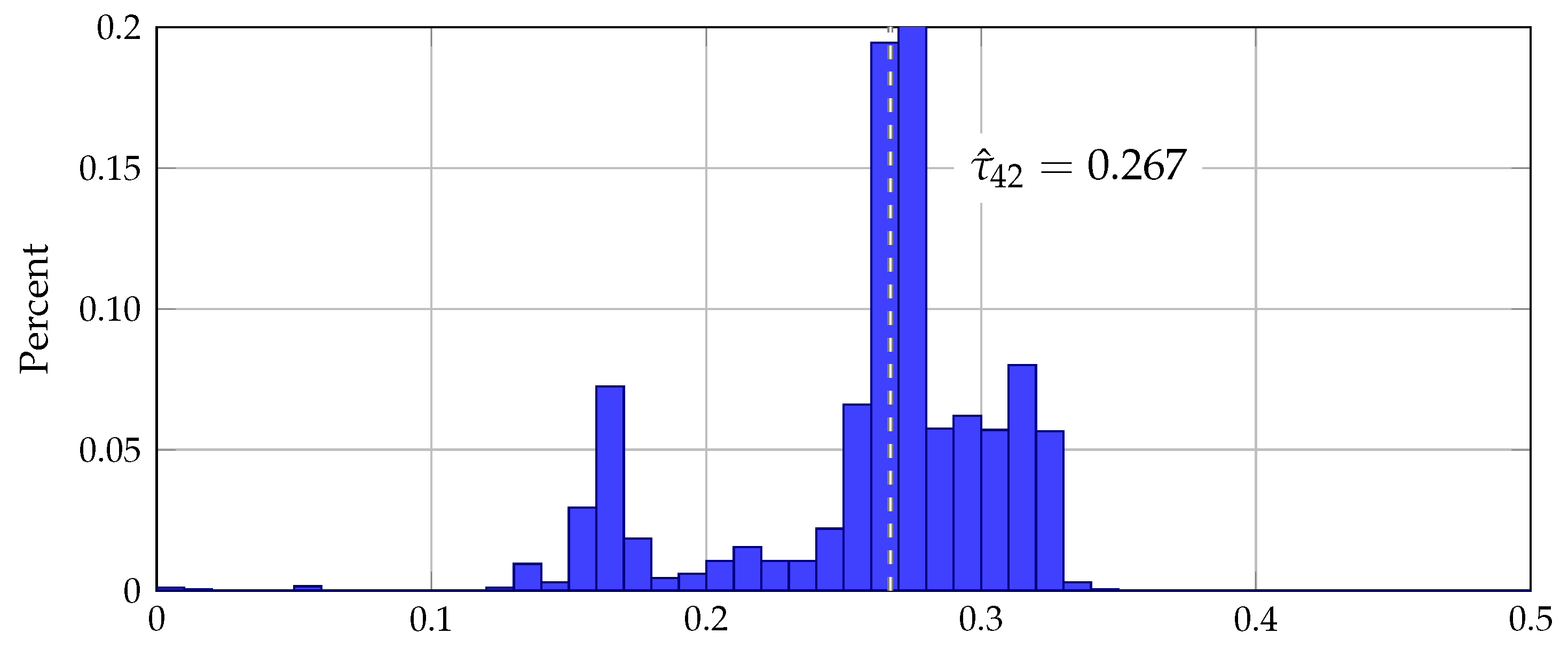
Table 1.
Payoff tables.
| Sender Payoffs | Receiver Payoffs | |||||||||
|---|---|---|---|---|---|---|---|---|---|---|
| Action Choice | State | State | ||||||||
| 43 | 7 | −32 | −72 | −115 | 100 | 75 | 43 | 7 | −32 | |
| 75 | 43 | 7 | −32 | −72 | 75 | 100 | 75 | 43 | 7 | |
| 100 | 75 | 43 | 7 | −32 | 43 | 75 | 100 | 75 | 43 | |
| 75 | 100 | 75 | 43 | 7 | 7 | 43 | 75 | 100 | 75 | |
| 43 | 75 | 100 | 75 | 43 | −32 | 7 | 43 | 75 | 100 | |
Table 2.
Informational content and distribution of messages across treatments.
| Precise Messages | State from which Sent ( | Frequency | ||||
| Base Treat | Rich Treat | % Base | % Rich | p | ||
| 1.81 | 2.50 | 0.278 a | 0.06 | 0.02 ** | 0.022 b | |
| 2.33 | 2.50 | 0.618 a | 0.11 | 0.03 *** | <0.001 b | |
| 2.43 | 2.29 | 0.771 a | 0.14 | 0.08 ** | 0.020 b | |
| 2.53 | 3.36 ** | 0.009 a | 0.18 | 0.07 *** | <0.001 b | |
| 3.28 | 3.58 * | 0.052 a | 0.51 | 0.34 *** | <0.001 b | |
| Imprecise Messages | State from which Sent () | Frequency | ||||
| Rich Treat | p | % Rich | p | |||
| 2.34 | 0.823 c | 0.07 | 0.703 d | |||
| 2.45 | 0.794 c | 0.10 | 0.170 d | |||
| 3.16 *** | 0.002 c | 0.29 *** | <0.001 d | |||
a and c: p values from two-sided Mann–Whitney U test comparing distribution of s from which m originated between treatments for precise messages a, or for all messages of same expected value b. b and d: p values from Fisher’s exact tests comparing frequency of precise m b or all messages of same expected value d. *: Significant at 0.1 level. **: Significant at 0.05 level. ***: Significant at 0.01 level.
Table 3.
Responses to messages.
| Precise Messages | Action Choice () | Optimal a | |||
| Base Treat | Rich Treat | p | Base | Rich | |
| 1.94 | 1.60 | 0.174 a | 1 | 2 | |
| 2.30 | 2.57 | 0.353 a | 2 | 2 | |
| 2.27 | 2.35 | 0.587 a | 2 | 2 | |
| 2.91 | 3.03 | 0.655 a | 2 | 3 | |
| 3.47 | 3.79 *** | 0.004 a | 3 | 4 | |
| Imprecise Messages | Action Choice () | Optimal a | |||
| Rich Treat | p | Rich | |||
| 2.07 | 0.440 b | 2 | |||
| 2.71 ** | 0.043 b | 2 | |||
| 3.10 | 0.159 b | 3 | |||
a and b: p values from two-sided Mann–Whitney U test comparing distribution of a for precise messages across treatments a or for base treatment messages to imprecise messages of the same expected value b. Optimal a values are a(m) that would have maximized expected payoff in the treatment. **: Significant at 0.05 level. ***: Significant at 0.01 level.
Table 4.
Base treatment message and action predictions (Proposition 1).
| State | Message | ||||||
|---|---|---|---|---|---|---|---|
| 1 | 3 | 2 | 1 | 1 | 1 | ||
| 2 | 4 | 5 | 2 | 2 | 1 | ||
| 3 | 5 | 5 | 3 | 1 | 1 | ||
| 4 | 5 | 5 | 4 | 2 | 2 | ||
| 5 | 5 | 5 | 5 | 4 | 4 | ||
†: For L5S and higher senders, there is a cutoff such that for λ > , m(1) = 5. ††: If λ < 1.46, then for L3S, m(2) = 4. ⋆: If λ < , then for L4R, a(2) = 2.
Table 5.
Rich treatment message predictions (Propositions 2 and 3).
| State | ||||||
|---|---|---|---|---|---|---|
| 1, | 3, | 1, | ||||
| 2, , | 4, | 5 | 2, , | |||
| 3, , , | 5 | 5 | 3, , , | |||
| 4, , | 5 | 5 | 4, , | 4 | ||
| 5, | 5 | 5 | 5, | 5 | 5 | |
†: If λ < 2.73 (respective of λ < 1.88), then L3S (L3S + L4S) send m(1) = {2,3,4} and m(2) = {3,4,5}. ††: If h is beneath an λ-dependent cutoff, L4S and higher send m(1) = {3,4,5} and m(2) = 5. ⋆: If h < 36, then if h is beneath a λ-dependent cutoff, L4S and higher send m(4) = 5.
Table 6.
Rich treatment action predictions (Proposition 4).
| Precise Message | Imprecise Message | ||||||
|---|---|---|---|---|---|---|---|
| 1 | 1 | 1 | 2 | 1 | 1 | ||
| 2 | 2 | 2 | 3 | 2 | 2 | ||
| 3 | 1 | 1 | 4 | 3 | 3 | ||
| 4 | 2 | 2 | |||||
| 5 | 4 | 4 | |||||
∘: If < 1/3, then if λ is greater than a -dependent cutoff, for L3R and higher, a({2,3,4}) = 1. ▴: If λ is greater than a -dependent cutoff, for L5R and higher, a({3, 4, 5}) = 2.
Table 7.
Parameter estimates.
| (1) | (2) | (3) | (4) | (5) | |
|---|---|---|---|---|---|
| Combined | Rich | Base | Senders | Receivers | |
| Treatments | Treatment | Treatment | Only | Only | |
| 3.294 | 2.722 | 3.63 | 3.381 | 2.712 | |
| [2.722, 3.79] | [2.419, 3.659] | [3.047, 4.5] | [2.341, 3.998] | [2.244, 3.387] | |
| 0.267 | 0.209 | 0.077 | 0.274 | 0.175 | |
| [0.132, 0.316] | [0.015, 0.298] | [0.0, 0.399] | [0.0, 0.321] | [0.0, 0.967] | |
| 0.027 | 0.029 | 0.025 | 0.026 | 0.03 | |
| [0.023, 0.034] | [0.024, 0.036] | [0.02, 0.033] | [0.022, 0.032] | [0.02, 0.04] | |
| n | 1384 | 848 | 536 | 692 | 692 |
| −2045.688 | −1379.507 | −660.605 | −1066.303 | −977.101 | |
| 4113.075 | 2779.243 | 1340.062 | 2152.226 | 1973.821 |
Maximum likelihood estimates of mean steps of thinking () and share of players with utility from honesty h = 42 (), where 95% BCa confidence intervals are reported beneath estimates.
Table 8.
Predicted mean distances of messages from state () and actions from message () from calibrating model with alternate message spaces and parameter estimates from base or rich language treament behavior.
Table 8.
Predicted mean distances of messages from state () and actions from message () from calibrating model with alternate message spaces and parameter estimates from base or rich language treament behavior.
| Counterfactual | ||
|---|---|---|
| Base treatment actual data | 1.52 | 1.30 |
| Base message space, base honesty, base rationality | 1.46 | 1.28 |
| Rich message space, base honesty, base rationality | 1.30 | 1.33 |
| Base message space, rich honesty, base rationality | 1.42 | 1.27 |
| Base message space, base honesty, rich rationality | 1.37 | 1.08 |
| Rich message space, rich honesty, base rationality | 1.25 | 1.25 |
| Base message space, rich honesty, rich rationality | 1.31 | 1.06 |
| Rich message space, base honesty, rich rationality | 1.23 | 1.14 |
| Rich message space, rich honesty, rich rationality | 1.16 | 1.05 |
| Rich treatment actual data | 1.22 | 0.98 |
Publisher’s Note: MDPI stays neutral with regard to jurisdictional claims in published maps and institutional affiliations. |
© 2022 by the author. Licensee MDPI, Basel, Switzerland. This article is an open access article distributed under the terms and conditions of the Creative Commons Attribution (CC BY) license (https://creativecommons.org/licenses/by/4.0/).
Share and Cite
MDPI and ACS Style
Wood, D.H. Communication-Enhancing Vagueness. Games 2022, 13, 49. https://doi.org/10.3390/g13040049
AMA Style
Wood DH. Communication-Enhancing Vagueness. Games. 2022; 13(4):49. https://doi.org/10.3390/g13040049
Chicago/Turabian StyleWood, Daniel H. 2022. "Communication-Enhancing Vagueness" Games 13, no. 4: 49. https://doi.org/10.3390/g13040049
Note that from the first issue of 2016, this journal uses article numbers instead of page numbers. See further details here.