Article

A Sparse Analysis-Based Single Image Super-Resolution

1
Department of Electrical and Computer Engineering, Science and Research Branch, Islamic Azad University, 14778-93855 Tehran, Iran
2
Department of Electrical and Computer Engineering, Isfahan University of Technology, 84156-83111 Isfahan, Iran
*
Author to whom correspondence should be addressed.
Computers 2019, 8(2), 41; https://doi.org/10.3390/computers8020041
Submission received: 1 May 2019 / Revised: 22 May 2019 / Accepted: 25 May 2019 / Published: 27 May 2019

Abstract

:
In the current study, we were inspired by sparse analysis signal representation theory to propose a novel single-image super-resolution method termed “sparse analysis-based super resolution” (SASR). This study presents and demonstrates mapping between low and high resolution images using a coupled sparse analysis operator learning method to reconstruct high resolution (HR) images. We further show that the proposed method selects more informative high and low resolution (LR) learning patches based on image texture complexity to train high and low resolution operators more efficiently. The coupled high and low resolution operators are used for high resolution image reconstruction at a low computational complexity cost. The experimental results for quantitative criteria peak signal to noise ratio (PSNR), root mean square error (RMSE), structural similarity index (SSIM) and elapsed time, human observation as a qualitative measure, and computational complexity verify the improvements offered by the proposed SASR algorithm.

1. Introduction

1.1. Background

Super resolution (SR) is a remarkable topic related to digital-image processing research. A hardware upgrade is the traditional solution to enhancing resolution, but is expensive in almost all cases. As a software-based technology, SR is an inexpensive and effective image processing technique. Many SR techniques have been proposed, including single-image super-resolution (SISR), which reconstructs a single low resolution (LR) image into a high resolution (HR) output image.
Conventional SISR techniques can be categorized into three classes. The first are interpolation-based techniques [1,2], which are the simplest solutions to the SISR problem. Bi-cubic and bilinear algorithms are the most well-known techniques in this category. Although their ringing and blocking effects are remarkable, simple structure and low complexity implementation are their main advantages. The second category comprises reconstruction-based techniques [3,4,5,6]. They deal with SR as an inverse problem. Their cost function has a general term for adapting HR and LR images and a regularization scheme to ensure better matching between the HR and LR images. Suresh et al. [6] used an adaptive edge detector as a regularization term in order to preserve edges and sharp image details. In a similar approach, Chen et al. [7] used a Tikhonov regularization term. Although most existing efforts in this category have worked well for small magnification factors, their performance decreases at larger magnification factors.
The third category of SISR algorithms is learning-based techniques [8,9,10,11,12,13]. These use a training dataset that includes HR–LR image pairs, and are based on a construction scheme for HR–LR databases called a dictionary. The extracted HR–LR image patches that have common features feed the dictionary. In HR image reconstruction, the LR patch closest to the input LR patch is found in the LR learned database. Its corresponding HR patch is then extracted and the resulting HR patches are merged to reconstruct the desired HR output image. These methods offer improved performance at a wide range of magnification factors and better quality in some image classes.
Training an effective HR–LR dictionary is a crucial stage in such algorithms. The sparse decomposition model has been used to propose SR algorithms based on dictionary learning techniques [10,11,12,13]. The sparse synthesis model assumes that each HR–LR image patch is composed of a few atoms from a learned HR–LR dictionary. The alternative sparse analysis model has been rarely examined for use in the SR field. In this study, we propose sparse analysis HR–LR operator learning and present a new approach to SISR.

1.2. Prior Work

Many SISR techniques have been proposed based on sparse coding and dictionary learning [10,11,12,13,14,15,16]. Yang et al. [11] proposed the first algorithm, which is known as SCSR. Their method was based on the sparse-synthesis model, which relies on the same sparse representation vector for each HR image patch and its corresponding LR patch in the HR–LR dictionary. HR–LR dictionary learning and HR image reconstruction were two main stages of these algorithms. In the first stage, the K-SVD dictionary learning method [17] has been modified for the HR–LR dictionary pair leaning by many authors. K-SVD is a dictionary learning algorithm based on K-means clustering and SVD matrix decomposition. It stands for K-means in addition to singular value decomposition [17].
Yang et al. proposed joint dictionary learning [12] and coupled dictionary learning [10] for the SCSR technique. Zeyde et al. [13] modified the SCSR algorithm to reduce the computational complexity and simplify HR dictionary learning using a single-image scale-up technique (SISU). Zhang et al. [14] proposed a dual dictionary-learning SR algorithm consisting of primary dictionary learning and residual dictionary learning to restore the main frequency detail and the residual frequency detail, respectively.
Chen et al. [7] took into account the differences in the structure of the patches and proposed the classified SR technique for smooth and non-smooth regions. They used bi-cubic interpolation for the smooth regions, and SR was implemented using the dictionary learning method for the non-smooth regions. Dong et al. [18] proposed the non-locally centralized sparse representation (NCSR) model to suppress the sparse coding noise in image restoration algorithms, such as SR [18]. Timofte et al. [19] combined sparse learned dictionaries with the neighbor embedding method and proposed the anchored neighborhood regression (ANR)method. Zhang et al. [20] proposed the adaptive mixed samples ridge regression (AMSRR) to effectively optimize learned dictionaries. Lu et al. [21] utilized the sparse domain selection method and achieved accurate and stable HR image recovery. Naderahmadian et al. modified the dictionary update step in online dictionary learning [22]. Other algorithms that have been proposed include classified dictionaries [23], sub-dictionary learning [24], and solo dictionary learning [25].
These SR algorithms are based on the assumption that each patch of the image can be restored as a linear combination of a few columns from a trained over-complete dictionary. Recently, a different model, sparse analysis, has been proposed [26] as a powerful alternative model for signal processing problems. Extensive research has focused on the high competency of the sparse analysis model [27,28,29]. Ning et al. [30] proposed an SR algorithm using iterative refinement and the analysis sparsity model in the Lab color space. Hawe et al. [31] proposed an algorithm for learning an analysis operator based on lp-norm minimization on the set of full rank matrices and implementation of the conjugate gradient method on manifolds. They considered the importance of suitable sparse analysis operators on output image quality. Nevertheless, it seems that the sparse analysis model has more potential for SR problems and requires further attention.

1.3. Contribution

Although synthesis-based sparse HR–LR dictionary learning methods have been studied extensively in SR algorithms, the analysis-based sparse model is an alternative model. We propose a coupled HR–LR sparse analysis operator that exploits mapping between HR–LR image patches. In addition to the use of patch-ordering total variation measures, we propose a novel sparse analysis operator learning method in the patch selection phase. In this way, the HR–LR patch pairs are trained based on image texture complexity, resulting in more-efficient HR–LR sparse analysis operators being trained.
We show that the proposed approach improves the quality of reconstructed HR images, as well as reducing the complexity of dictionary learning. Our experimental results show that the proposed method is comparable to state-of-the-art methods, both qualitatively and quantitatively. The main contributions of this paper are:
  • a novel SR technique is proposed for mapping between HR–LR patches based on HR–LR sparse analysis operators;
  • a new sparse operator learning method is proposed in the patch selection stage that considers image texture complexity;
  • the computational complexity of the algorithm is less than in previous approaches;
  • the proposed SASR results perform better in comparison with state-of-the-art and classic interpolation-based methods (bicubic SR, SCSR [12], SISU [13], ANR [19], GR [19], NE + LS [19] and GOAL [31], AMSRR [20], and SDS [21]).

1.4. Organization

The remainder of the paper is organized as follows. The proposed sparse analysis SR method is described in detail in Section 2. Section 3 presents experiments on the performance of the proposed SASR method in comparison with the bi-cubic SR, SCSR [12], SISU [13], ANR [19], GR [19], NE + LS [19], GOAL [31], AMSRR [20], and SDS [21] methods. The paper is concluded in Section 4.

2. Proposed Sparse Analysis-Based SR Algorithm (SASR)

This work aims at establishing a SR algorithm based on sparse analysis theory. We initially modify the sparse analysis operator learning algorithm by selection of an informative patch from learning images and then propose a novel SR algorithm based on coupled sparse analysis operators.

2.1. Sparse Analysis Model

In the conventional sparse synthesis model, image patch x R m is said to be “k-sparse” if it can be represented by a linear combination of k atoms from the over-complete dictionary D m × n as
x = D α s s . t : α s 0 0 = k .
where s is the sparse synthesis representation of x .
In the sparse analysis model, as an alternative model to the sparse synthesis model, an image patch is said to be l-cosparse if it produces a sparse vector when it is analyzed with a sparse analysis operator Ω n × m :
α A = Ω x s . t : α A 0 0 = m l .
While D is square and invertible, the two models are equivalent. In contrast, for a long time, the over-complete case of D and Ω were confused and were even considered to be equivalent. Elad et al. [26] considered the algebraic similarity between the two models, and showed that there is a surprising difference between them for over-complete dictionaries and operators.
Based on the assumption that an image patch can be restored as a linear combination of atoms from an over-complete dictionary, many algorithms have been proposed that aim to solve inverse problems regularized with the sparse-synthesis model. Given the observation that y = M x , where M R m × d is a linear observation matrix, the optimization formulation of these two inverse problems can be represented as
x ^ = arg min x = α s 0 0 s . t : M D α s y 2 2 ε ,
and
x ^ = arg min x = Ω x 0 0 s . t : M x y 2 2 ε .
Elad et al. [26] showed that if Ω = D (the pseudo-inverse of D ), the solutions of both the synthesis and analysis models are substantially different in the general over-complete case. In addition, they showed that the two formulations refer to very different models, and the analysis is much richer and may lead to better performance in various applications.

2.2. Image SR Using Coupled Sparse Analysis Operators

Sparsity has been used as an effective regulator for the ill-posed SISR problem. The core of traditional sparse representation-based SR is employment of the same sparse synthesis vector for corresponding HR and LR patches over the HR and LR learned dictionaries. Whereas sparse analysis has been successfully applied to many inverse problems in signal processing, we applied it to the SR problem. In our setting, we work with two coupled sparse analysis operators: Ω h for high resolution patches, and Ω l for low resolution ones. Because the basic assumption is the same sparse analysis vector for both HR and LR patches with respect to their analysis operators, the sparse analysis vector for LR patches is used directly to recover the corresponding high resolution patches for the HR analysis operator. Learning the HR–LR patch pair selection is the first step in the operator learning phase, and learning patch pair selection plays an important role in such methods. In this way, all patches extracted from each image are ordered based on structural similarity using a greedy algorithm. Next, the total variation measure is used to evaluate texture complexity and select a number of informative patches in each learning image. Figure 1 summarizes the proposed SASR algorithm.

2.2.1. Coupled Sparse Analysis Operator Learning

(a) Patch Selection Based on Ordering
Let Y be an image of size N 1 × N 2 and { y k } indicate the kth overlapping patch having size n × n . In the first stage, we extract all possible patches from the image. Assuming that each patch is a point in space R n , the goal is to reorder the patches so as to minimize the total variance (TV) measure:
{ y k } T V = j = 2 N 1 × N 2 y j y j 1 2 2 .
The smoothness of the ordered patches { y k } o can be measured using the TV. Minimizing the { y k } o T V results in the ordering of all extracted patches { y k } based on a structural similarity measure. We chose a simple approximate solution, which was to start from a random point and then continue from each patch y i to its nearest neighbor y j with a Euclidean distance similarity measure. TV minimization of patches using the proposed patch ordering is summarized in Algorithm 1.
Algorithm 1: Proposed patch ordering based on structural similarity
Task: Reorder the image patches { y k }
Parameters: We are given n × n image patches { y k } and distance function ω.
Let be the set of indices of all overlapping n × n patches extracted from the image.
Initialization:
Choose random index i A .
Set r = 1 , Ω ( r ) = { i } ,   Λ ( 1 ) = { i } .
Main iteration:
For j A
Find y j as the nearest neighbor to y i
If j A and j Λ
Set Ω ( r + 1 ) = { j } .
Otherwise:
Find y j as the nearest neighbor to y i such that A and   j Λ .
Set Ω ( r + 1 ) = { j } .
Output: Set Ω holds the proposed patch-based patch ordering.
We then calculate the total variation of { y k } and { y k } o using Equation (5). After calculating the TV measure for each image in the database, we assign the number of patches for each image proportional to its TV to the total TV of images as
m i = T V i j = 1 M T V j × M ,
where M is the total number of training patches and m i is the number of patches extracted from the ith image. After this step, we uniformly choose m i patches from each ordered image patch. Figure 2 shows examples of training images, and the results for the calculated TV measure, sampling step, and number of patches extracted for each image are shown in Table 1.
(b) Coupled Sparse Analysis Operator Learning
In this section, we introduce the proposed sparse analysis operator learning method, which trains the coupled Ω l and Ω h operators for the HR and LR patches. Sample set K contains training image patch pairs P = { x k , y k } k = 1 K , where X = { x k } k = 1 K are the selected high resolution patches and Y = { y k } k = 1 K are the corresponding low resolution patches. At this stage, the main goal is to learn coupled sparse analysis operators { Ω h , Ω l } , so that the sparse analysis vector of each high resolution patch is the same as the sparse analysis vector of the corresponding low resolution patch:
α k = Ω h x k and α k = Ω l y k . { x k , y k } P , k = 1 , K .
The analysis K-SVD algorithm is applied to train the low resolution sparse analysis operator Ω l . In this operator training algorithm, Robinstein et al. [25] supposed that given training set Y = { y k } k = 1 K R n × K as K clean vectorized patches of the LR images, Z = { z k } k = 1 K R n × K is a noisy version of the patches contaminated with additive zero-mean white Gaussian noise. They proposed the analysis K-SVD algorithm to find Ω R h × n , which forces the sparse analysis vector Ω y k to be sparse for each y i . They formulated an optimization task for the learning process as:
f ( Ω l , y k ) = min 1 2 Ω l , z k Ω l y k 0 0 + λ y k z k 2 2 .
Considering the constraint that each HR patch and its corresponding LR patch has the same sparse analysis vector with respect to the HR and LR sparse analysis operators, the LR training patches are analyzed by Ω l to obtain the sparse analysis vectors by k = Ω l y k . Therefore, for high resolution sparse analysis operator Ω h , we should have:
α k = Ω h x k ,
The solution of the problem is given by the following pseudo-inverse expression:
Ω h = A X = A X T ( X X T ) 1 ,
where matrix X is constructed with the selected high resolution training patches as its columns, and A contains sparse analysis vector k for paired low resolution patches over Ω l as its columns.

2.2.2. HR Image Reconstruction

Given LR image Y R N 1 × N 2 , we establish an SR sparse analysis method for reconstructing HR image X R f N 1 × f N 2 , where f is the magnification scale. First, we extract all LR patches by raster scanning Y = { y k } R n × n , where n is the size of the LR patches. Because sparse analysis vectors for high and low resolution patch pairs must have the same corresponding operators, we have:
α k Ω l x k Ω h y k .
In order to restore x k from y k , the LR sparse analysis operator is first applied to the LR patch to obtain vector α . Next, α is applied to the HR sparse analysis operator to obtain HR image patch x k using Ω h t α . After recovering all the HR image patches, a complete HR image X can be constructed by merging all these HR image patches by averaging the overlapping regions between adjacent patches. Because of the noise, and according to Equation (11), the reconstructed HR image may not exactly satisfy the observation model between the HR and LR images ( Y = M X ), where M is a linear observation model for downsampling and blurring. In order to enhance the output HR image, the regression output is refined as follows:
X * = arg min X Y M X 2 + c X X 0 2
where X 0 is the initial reconstructed HR image, the first term represents the reconstruction error and the second term recovers an image close to X 0 . Using gradient descent, optimal solution X * can be obtained as the final recovered HR image [12] as
X t + 1 = X t + τ { M T ( Y M X t ) + ( X t X 0 ) } .
where X t is the estimate of the high-resolution image after the t-th iteration and τ is the step size of the gradient descent.

3. Experimental Results

3.1. Test Setup

To evaluate the efficiency of the proposed SASR algorithm, it was compared with the following classic and state-of-the-art methods: bicubic interpolation, SCSR [12], SISU [13], ANR [19], GR [19], NE + LS [19] GOAL [31], AMSRR [20], and SDS [21]. All the source codes of the competing methods are publicly available on their authors’ webpages. For fair comparison, care was taken to ensure that the parameters used in the methods were similar. Because the first step in all learning-based SR algorithms is to select a dataset, all algorithms were tested on the same dataset. The HR and LR sparse analysis operators were trained using the dataset proposed by Yang et al. [12] (http://www.ifp.illinois.edu/~jyang29/). These HR images were down-sampled by bicubic interpolation to generate HR–LR image pairs for the training phase. To test the proposed algorithm, we took two standard datasets, SET14 (number of images = 14) and SET5 (number if images = 5), as testing images, which are two commonly used benchmark datasets in super-resolution literature. These images contain a nice mixture of details, flat regions, shading and texture. All testing was performed at a 3× magnification factor to validate the effectiveness of the proposed method. For patch selection in both the training and testing phases, our algorithm used 3 × 3 HR–LR patches with a two-pixel overlap.
All of the experiments were performed using MATLAB R2014a on an Intel (R) Core (TM) i5-M 460 @2.53 GHz machine with 4 GB of RAM.
The performance of the proposed algorithm was evaluated for root mean square error (RMSE), peak signal-to-noise ratio (PSNR), structural similarity index (SSIM), and running time between the luminance channels of the original and restored images. PSNR is defined as
P S N R ( X , X ^ ) = 10 log 10 255 2 M S E ( X , X ^ )
where X is the original HR image of size M × N , X ^ is reconstructed HR image, and M S E ( X ,   X ^ ) denotes the mean square error between X   and   X ^ , which is defined as
M S E ( X , X ^ ) = 1 M N i = 1 M j = 1 N ( X i , j X ^ i , j ) 2
RMSE is the square root of the MSE of Equation (14). Although, these two criteria have been very often used by SR researchers, they do not represent the human visual system very well. Therefore, another form of measure, such as structural similarity measure (SSIM), has also been used in SR algorithms. SSIM measure is defined as:
S S I M = ( 2 μ X μ X ^ + C 1 ) ( 2 σ X X ^ + C 2 ) ( μ X 2 + μ X ^ 2 + C 1 ) ( σ X 2 + σ X ^ 2 + C 2 )
where C 1 and C 2 are constants, μ X and μ X ^ are the mean of X and X ^ , respectively, and σ X and σ X ^ are the standard deviation of original and reconstructed images, respectively.
Because the human visual system is more sensitive to changes in the luminance channel, an LR color image first was transformed to YCbCr color space, then all SR methods were only applied to the luminance channel. The chromatic channels were reconstructed by bicubic interpolation, as is commonly performed in SR algorithms.

3.2. Results

We quantitatively and qualitatively evaluated the performance of the proposed method in comparison with bicubic interpolation, the SCSR [12], SISU [13], ANR [19], GR [19], NE + LS [19], GOAL [29], AMSRR [20], and SDS [21] methods. The sparse representation-based methods (SCSR [12] SISU [13]) and regression-based methods (ANR [19], GR [19], and NE + LS [19]) were used as for baseline methods. Three methods (AMSRR [20], SDS [21], and GOAL [29]) were used as for the state-of-the-art methods. Table 2, Table 3 and Table 4 show the quantitative comparison for the PSNR, RMSE, and SSIM measures. These tables reveal that the proposed SASR method can possess better performance compared with some state-of-the-art methods, and gained average improvements of 0.07 dB in PSNR, 0.14 in RMSE, and 0.0007 in the SSIM criteria.
Figure 3 and Figure 4 show the effectiveness of the proposed method. Figure 3 and Figure 4 present the image super-resolution results of all methods for the “Butterfly” and “Face” images at 3× magnification. For more precise comparison, specific zoomed scenes are provided. We observed that the bicubic and GR [19] methods tended to generate blocking and ringing artifacts. Although the SCSR [12], SISU [13], ANR [19], NE + LS [19], GOAL [29], AMSRR [20], and SDS [21] methods improved the visual details and edges, it can be seen that the proposed SASR algorithm had more acceptable performance when reconstructing sharp edges, and showed more detail compared to the other algorithms.
Although the objective quality of a few HR images obtained by the proposed method had a slight advantage over the other methods, the average quantitative evaluations of the proposed method are competitive to those of the others.
According to Table 5, the elapsed time of our algorithm is comparable with GR [19] and ANR [19], while its performance was much faster than other compared algorithms. Although in terms of elapsed time our proposed algorithm was not the fastest method, it achieved satisfactory results. According to Table 5, in terms of elapsed time, the proposed method was faster than SCSR [12], SISU [13], NE + LS [19], and AMSRR [20], while it was comparable with GR [19].
To compare the computational cost of the proposed and SCSR [12] methods, an image patch size of 5 × 5 was used for LR patches, and HR patches were obtained by implementing four feature extraction filters in order to extract high frequency details. Accordingly, after vectorization, LR patches with dimensions of 25 × 1 and HR patches with dimensions of 100 × 1 were obtained, leading to an LR dictionary with dimensions of 25 × 1024 and an HR dictionary with dimensions of 100 × 1024 . In the SISU method proposed by Zeyde et al. [13], the HR patch dimension decreased from 100 × 1 to 30 × 1 after implementing a dimension reduction algorithm. The ANR [19], GR [19], and NE + LS [19] methods followed Zeyde et al. [13].
GOAL [29] is based on a sparse analysis model and uses a geometric conjugate gradient method on the oblique manifold to solve the optimization task. The performance of the analysis approach can be further increased by learning the particular operator with regard to the specific problem or employing a specialized training set [31]. However, in the proposed SASR method, selected training patches were obtained from the patches having a size of 3 × 3 , and they were ordered by the proposed simple algorithm, leading to LR and HR dictionaries with dimensions of 9 × 1024 . Therefore, the structure of the proposed SASR method was simpler in the learning phase. Moreover, because the patch extraction method should be the same at the learning and reconstruction phases, this difference can also be observed in the HR image reconstruction stage. In the reconstruction phase, other methods have used greedy algorithms, such as matching pursuit (MP) and orthogonal matching pursuit (OMP), to determine the sparse representation vectors for each low resolution image patch. In the proposed SASR method, sparse analysis vectors for LR image patches were obtained through two simple operations: calculation of the pseudo-inverse matrix and multiplication. Total evaluation for the quantitative criteria (PSNR, RMSE, SSIM), human observation as a qualitative measure, and elapsed time for computational complexity comparison verify the improvement of the proposed SASR algorithm.

4. Conclusions

We proposed a single-image super-resolution algorithm based on recent sparse analysis signal representation with coupled HR–LR sparse analysis operator learning. We showed that conventional sparse synthesis SR methods can be reformulated into sparse analysis operators. The proposed method, SASR, uses a new patch extraction method from the learning dataset with patch ordering and total variation measures. The proposed approach uses a new sparse matrix for analysis of the image, in contrast with other sparse super-resolution approaches, which are all synthesis-based approaches.
The experimental results show that the performance of the proposed algorithm is comparable to that of state-of the-art algorithms in terms of quantitative metrics and visual quality. Although in terms of elapsed time our proposed algorithm is not the fastest method, it achieves satisfactory results.
Although the performance improvement was revealed in the average results of empirical evaluation of our proposed method, there is a high potential for extending the theory of this approach in SR applications. In addition, the proposed method has the potential to be applied to de-noising and de-blurring problems. Further study will focus on optimizing the sparse analysis operator training process to improve reconstruction efficiency.

Author Contributions

V.A contributed conceptualizing, methodology and software, F.R and R.A. did validation and visualization.

Funding

This research received no external funding.

Conflicts of Interest

The authors declare no conflict of interest.

References

  1. Dai, S.; Han, M.; Xu, W.; Wu, Y.; Gong, Y. Soft edge smoothness prior for alpha channel super resolution. In Proceedings of the 2007 IEEE Conference on Computer Vision and Pattern Recognition, Minneapolis, MN, USA, 17–22 June 2007. [Google Scholar]
  2. Sun, J.; Xu, Z.; Shum, H. Image super-resolution using gradient profile prior. In Proceedings of the 2008 IEEE Conference on Computer Vision and Pattern Recognition, Anchorage, AK, USA, 23–28 June 2008. [Google Scholar]
  3. Farsiu, S.; Robinson, M.D.; Elad, M.; Milanfar, P. Fast and robust multi-frame super resolution. IEEE Trans. Image Process. 2004, 13, 1327–1344. [Google Scholar] [CrossRef] [PubMed]
  4. Hardie, R.C.; Barnard, K.J.; Armstrong, E.E. Joint MAP registration and high-resolution image estimation using a sequence of under sampled images. IEEE Trans. Image Process. 1997, 6, 1621–1633. [Google Scholar] [CrossRef] [PubMed]
  5. Jiang, J.; Hu, R.; Han, Z.; Lu, T. Efficient single image super-resolution via graph-constrained least squares regression. Multimed. Tools Appl. 2014, 72, 2573–2596. [Google Scholar] [CrossRef]
  6. Suresh, K.V.; Rajagopalan, A. A discontinuity adaptive method for super-resolution of license plates. In Computer Vision, Graphics and Image Processing; Kalra, P.K., Peleg, S., Eds.; Lecture Notes in Computer Science; Springer: Berlin, Germany, 2006; Volume 4338, pp. 25–34. [Google Scholar]
  7. Chen, H.; Jiang, B.; Chen, B. Image super-resolution based on patches structure. In Proceedings of the 2011 IEEE International Congress Image and Signal Processing, Shanghai, China, 15–17 October 2011; pp. 1076–1080. [Google Scholar]
  8. Freeman, W.T.; Jones, T.R.; Pasztor, E.C. Example-based super-resolution. IEEE Comput. Graph. Appl. 2002, 22, 56–65. [Google Scholar] [CrossRef] [Green Version]
  9. Gao, X.; Zhang, K.; Tao, D.; Li, X. Image super-resolution with sparse neighbor embedding. IEEE Trans. Image Process. 2012, 21, 3194–3205. [Google Scholar] [PubMed]
  10. Yang, J.; Wang, Z.; Lin, Z.; Cohen, S.; Huang, T. Coupled dictionary training for image super-resolution. IEEE Trans. Image Process. 2012, 21, 3467–3478. [Google Scholar] [CrossRef] [PubMed]
  11. Yang, J.; Wright, J.; Huang, T.; Ma, Y. Image super-resolution as sparse representation of raw image patches. In Proceedings of the 2008 IEEE Conference on Computer Vision and Pattern Recognition, Anchorage, AK, USA, 23–28 June 2008. [Google Scholar]
  12. Yang, J.; Wright, J.; Huang, T.; Ma, Y. Image super-resolution via sparse representation. IEEE Trans. Image Process. 2010, 19, 2861–2873. [Google Scholar] [CrossRef] [PubMed]
  13. Zeyde, R.; Elad, M.; Protter, M. On single image scale-up using sparse-representations. In Proceedings of the 7th International Conference on Curves and Surfaces, Avignon, France, 24–30 June 2010; Lecture Notes in Computer Science. Springer: Berlin/Heidelberg, Germany, 2010; Volume 6920, pp. 711–730. [Google Scholar]
  14. Zhang, J.; Zhao, C.; Xiong, R.; Ma, S. Image super-resolution via dual-dictionary learning and sparse representation. In Proceedings of the 2012 IEEE International Symposium on Circuits and Systems (ISCAS), Seoul, Korea, 20–23 May 2012; pp. 1688–1691. [Google Scholar]
  15. Yeganli, F.; Nazzal, M.; Unal, M.; Ozkaramanli, H. Image super-resolution via sparse representation over coupled dictionary learning based on patch sharpness. In Proceedings of the 2012 IEEE European Modelling Symposium, Pisa, Italy, 21–23 October 2014; pp. 203–208. [Google Scholar]
  16. Wang, S.; Zhang, L.; Liang, Y.; Pan, Q. Semi-coupled dictionary learning with applications to image super-resolution and photo-sketch synthesis. In Proceedings of the 2012 IEEE Conference on Computer Vision and Pattern Recognition, Providence, RI, USA, 16–21 June 2012; pp. 2216–2223. [Google Scholar]
  17. Aharon, M.; Elad, M.; Bruckstein, A. A K-SVD: An algorithm for designing overcomplete dictionaries for sparse representation. IEEE Trans. Signal Process. 2006, 54, 4311–4322. [Google Scholar] [CrossRef]
  18. Dong, W.; Zhang, L.; Shi, G.; LI, X. Nonlocally centralized sparse representation for image restoration. IEEE Trans. Image Process. 2013, 22, 1620–1630. [Google Scholar] [CrossRef] [PubMed]
  19. Timofte, R.; De Smet, V.; Van Gool, L. Anchored neighborhood regression for fast example-based super-resolution. In Proceedings of the 2013 IEEE International Conference on Computer Vision, Sydney, Australia, 1–8 December 2013; pp. 1920–1927. [Google Scholar]
  20. Zhang, H.; Liu, W.; Liu, J.; Liu, C.; Shi, C. Sparse representation and adaptive mixed samples regression for single image super-resolution. Signal Process Image Commun. 2018, 67, 79–89. [Google Scholar] [CrossRef]
  21. Lu, W.; Sun, H.; Wang, R.; He, L.; Jou, M.; Syu, S.; Li, J. Single image super resolution based on sparse domain selection. Neurocomputing 2017, 269, 180–187. [Google Scholar] [CrossRef]
  22. Naderahmadian, Y.; Beheshti, S.; Tinati, M.A. Correlation based online dictionary learning algorithm. IEEE Trans. Signal Process. 2016, 64, 592–602. [Google Scholar] [CrossRef]
  23. Zhu, X.; Tao, J.; Li, B.; Chen, X.; Li, Q. A novel image super-resolution reconstruction method based on sparse representation using classified dictionaries. In Proceedings of the 2015 IEEE International Conference on Information and Automation, Lijiang, China, 8–10 August 2015; pp. 776–780. [Google Scholar]
  24. Yang, W.; Yuan, T.; Wang, W.; Zhao, F.; Liao, Q. Single-Image Super-Resolution by Subdictionary Coding and Kernel Regression. IEEE Trans. Syst. Man Cybern. 2017, 47, 2478–2488. [Google Scholar] [CrossRef]
  25. Juefei-Xu, F.; Savvides, M. Single face image super-resolution via solo dictionary learning. In Proceedings of the 2015 IEEE International Conference on Image Processing (ICIP), Quebec City, QC, Canada, 27–30 September 2015; pp. 2239–2243. [Google Scholar]
  26. Elad, M.; Milanfar, P.; Rubinstein, R. Analysis versus synthesis in signal priors. Inverse Problems 2007, 23, 947–953. [Google Scholar] [CrossRef]
  27. Rubinstein, R.; Peleg, T.; Elad, M. Analysis K-SVD: A dictionary-learning algorithm for the analysis sparse model. IEEE Trans. Signal Process. 2013, 61, 661–677. [Google Scholar] [CrossRef]
  28. Dong, J.; Wang, W.; Dai, W. Analysis SimCO algorithms for sparse analysis model based dictionary learning. IEEE Trans. Signal Process. 2016, 64, 417–431. [Google Scholar] [CrossRef]
  29. Seibert, M.; Wörmann, J.; Gribonval, R. Learning co-sparse analysis operators with separable structures. IEEE Trans. Signal Process. 2016, 64, 120–130. [Google Scholar] [CrossRef]
  30. Ning, Q.; Chen, K.; Yi, L. Image super-resolution via analysis sparse prior. IEEE Signal Process. Letters 2013, 20, 399–402. [Google Scholar] [CrossRef]
  31. Hawe, S.; Kleinsteuber, M.; Diepold, K. Analysis operator learning and its application to image reconstruction. IEEE Trans. Image Process. 2013, 22, 2138–2150. [Google Scholar] [CrossRef] [PubMed]
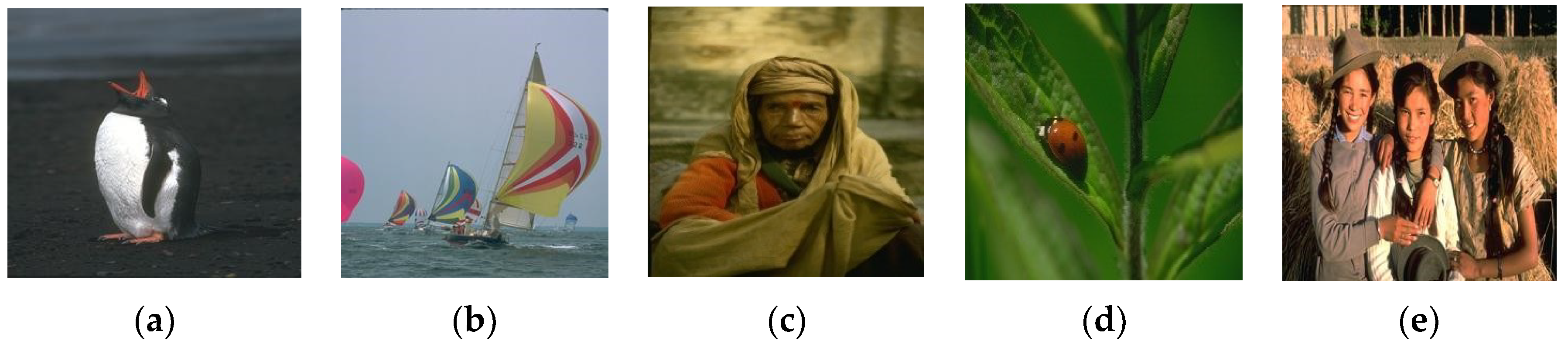
Figure 1. Architecture of proposed sparse analysis-based super-resolution algorithm.
Computers 08 00041 g001
Figure 2. Examples of training images used for patch selection. (a) Penguin, (b) boats, (c) old woman, (d) ladybug, and (e) girls.
Computers 08 00041 g002
Figure 3. SR results of the “Face” image with a magnification factor of 3X. Images from left to right and top to bottom: LR input image, original HR image, bicubic, SCSR [12], SISU [13], GR [19], ANR [19], NE + LS [19], GOAL [29], AMSRR [20], SDS [21], and our proposed SASR.
Computers 08 00041 g003
Figure 4. SR results of the “Butterfly” image with a magnification factor of 3X. Images from left to right and top to bottom: LR input image, original HR image, bicubic, SCSR [12], SISU [13], GR [19], ANR [19], NE + LS [19]), GOAL [29], AMSRR [20], SDS [21], and our proposed SASR.
Computers 08 00041 g004
Table 1. Total variance (TV) measure, sampling step, and number of extracted patches for sample images in Figure 2 (total number of training patches is 50,000).
ImageTotal VariationSampling StepNumber of Extracted Patches
Penguin940135044
Boats1248106696
Old woman167278974
Ladybird1047125621
Girls4409323,662
Table 2. PSNR (dB) of the reconstructed HR images with a magnification factor of m = 3.
LenaBarbaraZebraButterflyCatSailsCoastguardParrotPoolFaceAverage
Bicubic29.8026.9121.5624.5823.3325.7226.7930.6933.6233.8827.68
SRSC [12]30.8727.4023.1325.4823.7726.3826.8030.9434.8534.3128.39
SISU [13]31.0427.8623.1625.6023.8926.4427.3031.2035.2834.8528.66
GR [19]30.5627.5423.1425.6123.9726.3327.1531.0034.6134.7228.46
ANR [19]31.1127.8323.2825.7723.9326.5227.2331.2035.3234.9428.71
NE + LS [19]31.0827.7323.1425.6523.8626.4027.2430.1435.3834.8028.54
GOAL [29]31.2227.7923.1825.8324.1026.5527.2731.3035.4734.8928.76
AMSRR [20]31.4727.8523.2725.8224.1226.5627.1130.9135.3934.6528.71
SDS [21]31.6027.8023.2125.7223.9826.5127.0930.8834.7834.6628.62
Proposed SASR31.6827.8723.2425.9224.1926.4727.1331.1634.9634.6928.83
Table 3. RMSE of the reconstructed HR images with a magnification factor of m = 3.
LenaBarbaraZebraButterflyCatSailsCoastguardParrotPoolFaceAverage
Bicubic8.2411.4919.9815.0417.3713.1911.667.445.315.1511.48
SRSC [12]7.2810.8617.7713.5516.5112.2311.667.234.614.9010.66
SISU [13]7.1510.3117.7113.3716.2812.1411.007.014.384.6010.39
GR [19]7.5510.6917.7513.3516.1412.2911.197.174.734.6710.55
ANR [19]7.0910.3417.4613.1116.2112.0211.087.874.364.5610.41
NE + LS [19]7.1110.4617.7513.3016.3312.2011.077.024.334.6310.42
GOAL [29]7.0010.3917.6713.0215.8911.9811.276.934.294.5810.30
AMSRR [20]6.9510.5917.5113.0015.8612.2011.077.274.324.7010.34
SDS [21]6.7110.5217.5813.1116.2012.2211.167.304.504.7110.40
Proposed SASR6.649.2717.5412.8815.7212.0911.217.044.554.6910.16
Table 4. SSIM of the reconstructed HR images with a magnification factor of m = 3.
LenaBarbaraZebraButterflyCatSailsCoastguardParrotPoolFaceAverage
Bicubic0.84220.77370.69140.84120.70230.66030.60640.86120.95400.84770.7780
SRSC [12]0.85810.79760.74260.87160.74910.70600.61940.86070.95970.84900.8014
SISU [13]0.86990.81440.75010.87490.74990.71010.64220.87510.96550.86780.8120
GR [19]0.85920.79640.75490.87610.76290.71090.64280.87260.95850.86890.8103
ANR [19]0.87200.81240.75570.87930.75640.71600.64240.87900.96520.87060.8149
NE + LS [19]0.87010.80870.74780.87480.74850.71600.63970.87610.96560.86650.8114
GOAL [29]0.87450.80980.75100.88070.76270.71410.63420.87820.96510.86950.8139
AMSRR [20]0.87010.82910.75460.88080.76590.71650.64270.87250.96560.86110.8159
SDS [21]0.86980.82920.75410.87940.75640.71560.64230.87200.95560.86680.8141
Proposed SASR0.88070.82960.74700.87430.76690.70930.65880.87310.95980.86600.8166
Table 5. Average elapsed time of the reconstructed HR images with a magnification factor of m = 3.
BenchmarkProposed SASRSCSR [12]SISU [13]GR [19]ANR [19]NE + LS [19]AMSRR [20]GOAL [29]SDS [21]
Set 51.1092.112.500.530.7914.3440.5012.343.15
Set 141.1989.292.550.480.7115.9338.7012.933.06

