1. Introduction
Downsampling of 2D images is a technique employed in order to reduce the resolution of an input image. This is most helpful for reducing the storage size of images while preserving as much of their information as possible. Upsampling is the reverse process of the former, and it consists of obtaining an output image of a higher resolution than that of the input. In practice, the focus lies on obtaining a high confidence image—one that presents no unwanted artifacts and preserves high levels of detail.
The problem referenced throughout this paper is also known as interpolation, and it resides in inferring a continuous function from a discrete set of values. The interpolation problem is not a new one. Meijering [
1] describes the history of interpolation techniques from the Babylonian astronomers up to the modern adaptive and content-aware methods.
Research on interpolation techniques is of high value, especially in the medical imaging domain, as shown by Thevenaz et al. [
2], where the required quality and resolution of obtained images—such as magnetic resonance imaging (MRIs)—must be as high as possible. Reconstructions of non-uniformly sampled volumes, such as that of viruses, are also accomplished with the aid of interpolation. Some techniques such as CAD (computer-assisted diagnostics) and CAS (computer-assisted surgery) rely on certain resolution constraints, either for identifying patterns in diagnostics or for providing high fidelity imaging for specialists.
As pointed out by Meiijering et al. in [
3], the study of image interpolation in medical imaging research is of extreme importance for reconstructing accurate samples of CTs (computed tomography), MRIs, DSAs (digital subtraction angiography), and PETs (positron emission tomography).
Even though most of the research performed in regards to interpolation is tied to the medical imaging field, research has also been performed on various other types of images. The metrics used in either of them are dependent on several aspects regarding their application. Mitchell and Netravalli [
4] subjectively tested the effectiveness of their filtering techniques with many samples shown to multiple users. This way, they showed some thresholds and conditions that their proposed interpolation kernel must obey in order to be satisfying to the human eye.
More quantitative approaches in evaluating interpolation results are subject to active research. However, one can distinguish evaluation methods based on the frequency response of the image and on its spatial response. A survey conducted by Amanatiadis and Andreadis [
5] shows different approaches towards evaluating the quality of the interpolation algorithm in use. We note that Wang et al. [
6] argue that the classical usage of MSE (mean squared error) and PSNR (peak signal-to-noise ratio) as metrics for image quality assessment does not cover the localization of errors and fails to cover perceptual measurements based on the HVS (human visual system). Mughal et al. [
7] also discusses the usage of SSIM (structural SIMilarity) and proposes a weighted geometric mean from luminance, contrast, and structural similarity of different images. Wang et al. [
6] show that Weber’s law [
8] is respected with regards to the perceptual change in the visual stimulus introduced by the error signal against the original image. While SSIM is a significant quality assessment technique that involves human visual perception in the process of evaluating errors, it is still a 2D image of the spatial distribution of error with regards to the originally sampled 2D signal. For evaluation purposes, a scalar result quantifying the image quality globally is required. The MSSIM (mean structural SIMilarity) is also presented in [
6] as a means of globally describing the impact error signals on a 2D visible image. The author proposes the following formulation of the SSIM:
where:
The signals x and y are corresponding windows inside the original image,
is the mean of the signal x,
is the standard deviation of the signal x,
is the covariance of the two signals x and y,
and are two constants taken for stability purposes in the case where either term of the denominator is close to zero.
Al-Fahoum and Reza [
9] argue for a better method of quantifying image quality, stating that, even though MSE and its counterparts provide a good measurement of overall deviation from one image to another, they could provide a quantitative measurement for the edge intensity of an image, PEE (percentage edge error). They define this measurement as the difference between the ES (edge sharpness) of the original image and that of the processed image normalized by the ES of the original image
and
, where EI is the edge intensity of a given point. The procedure of determining the EI is further described in [
9] and takes into account edge intensities on both rows and columns. Al-Fahoum and Reza [
9] also propose a subjective quality index, the mean opinion score for characterizing the difference between two images on a scale from zero to five that they further utilize to show the degree of similarity between two images.
Another technique commonly employed in terms of evaluating the quality of the filters for both downsampling and upsampling is that of computing the response of the filter and comparing it to the ideal low-pass filter characteristics. In this concern, please note that an evaluation of an interpolation kernel is given by Schaum [
10], who shows the aforementioned properties of well-performing interpolation kernels.
Moller et al. [
11] propose a Taylor series approach to signal filter design, which aims at reconstructing derivatives and minimizing the error in the acception of Taylor series expansion of a given interpolated signal from its samples. Not only is interpolation used for upsampling/downsampling, but it is also used for applying Euclidean geometric transforms to different images in 2D. Thus, many of the envisaged interpolation techniques yield different results depending on the application (upsampling/downsampling, rotation).
Some surveys in the field of image interpolation convolution kernels are described by Meijering [
1] and usually take on a quantitative approach to measuring the quality of given transforms. Parker et al. [
12] present a first survey on the topic of interpolation that shows the results obtained by certain polynomial filters and analyzes their results in the time and frequency domain. In [
13], Lehman and Gonner continue with a survey regarding the common methods for the interpolation of medical images and analyze the size and shapes of their frequency response. They propose a means of measuring the quality of the interpolation using the normalized cross-correlation coefficient between the original image and the transformed and then with the reversed transformed applied to it. The higher this coefficient is, the better the result is. They also point out some key aspects regarding interpolation, the differences between interpolation and approximation methods, and they show the known integral-of-one principle of an interpolator, due to which the direct current component of the signal should be preserved as a consequence of the interpolation transform. In other words, Lehmann shows through several examples that, should the energy of the window function involved in the interpolation process be higher than the unit, then light areas of the image are bound to suffer from degradation, while a lower than unit total energy does more damage to the dark portions of the image.
Thevenaz et al. [
2] perform another survey and present several interpolation kernels, such as Meijering [
14], Schaum [
10], German [
15], Keys [
16], Dodgson [
17], and O-MOMS (optimal-maximal order minimal support) [
18,
19], while comparing them to the more classical ones based on the apodization of the sinc function.
Meijering [
3] perfects a survey on different interpolation methods while taking into account more window functions than his predecessors and presents his conclusions with regards to the RMSE (root mean squared error) between the undersampled and the upsampled images, focusing on medical images and evaluating the given kernels on various experiments (resampling, rotation, translation, etc.).
Sudheer [
20] presents a survey comprising multiple approaches towards image interpolation while keeping in mind the linear kernel-based approach and describing several other non-linear techniques for obtaining a super-resolution image from a normal resolution one.
Many other approaches other than using linear reconstruction kernels (interpolation functions) are described in [
21,
22,
23,
24,
25], to name just a few.
The purpose of the current paper is to present and evaluate some of the existing convolution-based interpolation methods. We aim to provide a comprehensive list of methods, classifying them based on their method and means to evaluate their behavior. In order to evaluate the quality of a given filter, computing and comparison of both MSE/PSNR and MSSIM are employed.
where:
is the original signal,
is the resampled image,
is the maximum value of the signal x.
In the case of a bi-dimensional signal (i.e., an image), the definitions in Equation (2) are similar.
The 2D resampling tests are applied on a significant dataset of images ranging from text, pictures, biological imagery, aerial views, textures, and artificial imagery. For this purpose, we use different databases described in
Section 4.
The underlying objective is the provision of an optimal filtering technique quality-wise on each given dataset. This paper’s further objective is providing means to choose an appropriate method for interpolation in more specialized applications, such as image compression (see
Section 6 for current and further development on the matter).
The rest of the paper is structured as follows: in the second section, the interpolation problem is defined, and the mathematical aspects of its workings are further detailed by providing the used formulas and notations that are used throughout this paper. In the third section, currently available methods are discussed and dissected in terms of linear interpolation methods (interpolation kernel approach), which are segregated into sinc-windowing techniques with the various window polynomial interpolation. At the end of the third section, insights into adaptive non-linear approaches towards interpolation are given in a succinct fashion. The fourth section consists of the results obtained on the described datasets and a comparison of the quality of the underlying filtering technology employed. Please note that only the interpolation kernel approach is evaluated, while the non-linear techniques succinctly described in the third section are not in the scope of the current paper. In the fifth section, the conclusions of this survey are presented with regards to the paper’s main objectives, while in the sixth section, further development opportunities are presented in regards to the paper’s main topic.
2. Problem Definition
This section comprises several theoretical considerations regarding the topic of downsampling and upsampling. Proving the theorems and lemmas involved throughout this section is out of the scope of this paper.
This section is structured such that in the first part, we give empirical qualitative criteria that are emphasized for the design of proper interpolation filters; the second describes a frequency domain approach. In the third part, we describe polynomial-based techniques, while in the fourth, we give some insights into the design of adaptive interpolation techniques.
In his thesis, Wittman [
21] describes the objectives of an interpolation technique while making the distinction between the desired visual characteristics and the computational stability criteria that ought to be accomplished in order to claim success over a resampling schema. In this paper, we enumerate through the properties proposed by Wittman and succinctly describe some of their meanings:
Geometric invariance—keeping geometrical information about the image subject
Contrast invariance
Noise—no supplementary noise addition to the original image
Edge preservation
Aliasing
Over-smoothing
Application awareness
Sensitivity to parameters
The theoretical support provided for this paper is inspired by Oppenheim’s classic book on discrete time signal processing [
26], as well as on the course by Serbanescu et al. [
27], especially with respect to the topic of multirate signal processing. An introductory text on wavelet analysis is provided in [
28] since numerous wavelet-based approaches to interpolation have been developed; an example in that concern is a paper by Nguyen and Milanfar [
29].
Let be a discrete time signal where x is a continuous time signal . We denote T the sampling rate of the signal x and let be its sampling frequency. We state that is the Z-transform of discrete-time sequence and denote this fact as , . Let us define the convolution of analog signals x and h as . In this respect, taking into account that a discrete-time signal x is the sampling of an original analog signal at sampling intervals , we now derive . Assuming that x is a bandlimited signal at the frequencies of , then by the Nyquist sampling theorem, one can obtain the original analog signal from the given samples if the sampling frequency .
Please note that from here on, the terms interpolation and decimation are used interchangeably with those of upsampling and downsampling, respectively. We define in
Figure 1 the schema described by Youssef in [
30] for the operation of downsampling/upsampling for a given 1D signal input:
In this schema, we take
a discrete time signal, the box
represents the operation of decimation by a factor of n, the box
the operation of interpolation by a factor of n, while the two
represent the filters used as decimation preprocessing and interpolation post-processing, respectively. The internals of the following boxes are described in terms of time and then frequency response. The decimator is described by the following transfer function:
and the interpolator by:
For simplicity, we assume that in our case.
The two aforementioned filters are low-pass filters, and their application on the input signal is a convolution operation. From the properties of the Z-transform, we find that , where and , x and h are discrete time signals.
Let be the Z-transform of the input signal . We deduce that , . However, since w is defined as zero on the odd indices, we have . We use in order to emphasize the frequency response (as far as the Fourier transform is concerned) of the chain of filters described above.
Following the reasoning of [
30], we state that the “useful” term in the above equation is precisely the first one and can consider that the second term appears because of the inherent aliasing nature of the high-frequency response. In order for the above frequency response of the entire system to be as close as possible to
X(
z) and in order to accomplish this desiderate, we argue that the first term of the above equation be as close as possible to
X(
z) while the second one be as close as possible to zero. In reality, it is impossible to accomplish this condition on the entire
range. Therefore, as described by [
30], one can deduce the following:
Theorem 1. In the ideal case, filters g and p are low-pass filters with pass-band equals to . In this situation, the signal preserves the highest possible range of low frequencies and keeps the aliasing distortion as close to zero as possible.
We observe that, as common grounds for building a signal interpolator, one must approximate (as well as possible) the shape of a low-pass filter. This is a consequence of the Nyquist theorem stated above. That being said, for a bandlimited signal, it is safe to assume that the analog signal from which it derives can be reconstructed exactly using an ideal low pass filter with cutoff frequency at .
The problems that arise using this generic signal processing approach reside in that, even though most of the natural images present the highest concentration of energy among the low-frequency components, there are several higher frequencies that get removed from the original image, which can cause loss of detail at the level of discontinuities in the image.
Another factor that forbids the use of ideal low-pass filters is that their impulse response is infinite in the time domain. Thus, the time-domain of the ideal low-pass filter is given by , where .
The shape of the sinc filter in the spatial domain against its shape in the frequency domain is shown in
Figure 2. We note that an ideal low-pass filter cannot be obtained, since the sinc function has infinite support. One can observe the ripples around the cutoff frequency of the frequency domain of the aforementioned plot; from these, one can deduce that even though a large support was indeed employed when writing the sinc function [−1000, 1000] with a sampling rate of 0.1, one cannot ensure ideal low-pass filtering for this design.
The general idea behind the design of frequency response-based filters is to try and approximate, as accurately as possible, the sinc function in the time domain while at the same time keeping the function in the FIR (Finite Impulse Response filter) constraints, since an infinite impulse response filter is not achievable in practice due to its infinite support and lack of causality (i.e., it takes into account many values from the future infinitely). In that respect, one can determine finite time computation of the convolution between the input signal and the convolution kernel, as well as come as close as possible to the ideal case described by the Nyquist sampling theorem.
As can be derived from
Figure 2, we note that, even though the impulse has a large enough support domain, it still presents malformations around the cutoff frequency. Therefore, using a simple sinc function cutoff (taking only a limited time domain for the function) yields bad results in terms of quality over the amount of computation necessary.
The method of choice for accomplishing the tradeoff between the number of samples taken into account, the resolution of the filter, as well as its behavior in the stopband, is the technique of windowing or apodization [
26]. A window is a function defined on the real numbers with the property that it is non-zero on a given interval
and is zero outside the named interval. We continue this section with a succinct presentation of the windowing techniques and the tradeoffs one has to accomplish in order to create an efficient—and in the meantime, qualitative—approximation for the sinc filter in the frequency domain.
A windowed-sinc kernel is a function defined as:
Transforming into the frequency domain, a multiplication becomes convolution. Therefore, any sharp discontinuities result in the existence of significant high-frequency components that propagate for the entire length of the signal, because and, reciprocally, .
Three criteria define a well-performing windowed-sinc filter:
Reduced roll-off—reducing the transition frequency difference between the passband and the stopband,
Low ripples in the passband and the in the stopband—the deviations from the ideal amplification one in the passband and respectively zero in the stopband are to be minimized in order to obtain closeness to the ideal filter,
Low energy in the stopband—that is to say, filters ought to produce most of their energy in the passband and close to zero in the stopband.
The most common windows employed in the field of finite impulse response filter design are the Hamming, the Blackman, and the Hanning windows. Many other windowing functions exist; they are described in
Section 3. However, in
Figure 3, we propose a comparison between a Hamming, a Hanning, and a Blackman window:
From
Figure 3, one can notice that the best performance in terms of stopband attenuation is obtained with the Blackman window. However, the fastest roll-off is obtained through a Hamming window, even though the latter has lower stopband attenuation. As a general rule in designing finite impulse response filters, one has to take into account the usage of a given function based on the underlying application. For example, in order to be able to better distinguish nearby frequencies, one should use the fastest transition filter in terms of passband to stopband roll-off. Such a window is the rectangular window filter or the mere truncating of the sinc function at a given sample.
These desiderates cannot be simultaneously accomplished. However, increasing the number of kernel samples usually reduces the roll-off and trades computation complexity for better filter approximation. Thorough explanations on the topic are offered in [
26,
31].
Appledorn [
32] has a different approach to signal interpolation that involves the use of the Gaussian symmetric interpolation kernel of zero mean and linear combinations of its derivatives in order to approximate several desired characteristics resembling those of the ideal sinc kernel in both frequency and time-domain. He also brings forward results regarding the performances obtained by his proposed method.
We describe the basics of polynomial interpolation. Polynomial interpolants for discrete samples of data have been employed since the early days in mathematics. Among the best-known methods for polynomial interpolation are ones that belong to Lagrange and Newton. In fact, the latter is more adapted for computer processing, since it provides an iterative means to computing further degrees without needing to recompute the entire polynomials [
33]. Important mathematicians also have their names related to polynomial forms of interpolation (Hermite, Bernstein, and Neville, to name a few).
For the purpose of this paper, we emphasize the specific image processing related matters taken into consideration. Besides the basic box and the linear interpolation kernel, there are other methods such as cubic interpolation, B-spline interpolation, piecewise symmetrical
n-th order polynomials [
14], and BC-splines [
4], etc.
Generalizing the concept of polynomial interpolation and keeping the smoothness between several samples of interpolated data, Meijering et al. [
14] manage to prove that a number of
n-2 continuous derivatives are required to be continuous at the knots in order to characterize the underlying polynomials with only one parameter
.
The theory of approximation comes as a handy tool for developing highly efficient yet well-behaved filters for the interpolation of data. The work of Thevenaz and Unser [
2,
34] provides the theoretical background for generalizing the interpolation problem with respect to the choice of more general approximation filters that are employed to perform interpolation with all the due restrictions and approximate arbitrary function of a given order. The proposed approaches employ a rewrite of an unknown function in a basis of approximating functions, as depicted in
, while imposing a secondary condition that the samples match at integer values. Meanwhile, in classical interpolation, the parameters
are precisely the samples of the initial function at integer nodes
and the supplementary condition that
and
. A highly revealing paper on the matter is presented in [
35], where examples of B-spline interpolation are also given.
The milder assumption resolves to solve a linear system of equations in order to find the exact coefficients
after the imposition of the condition that
. Furthermore, more efficient digital signal filtering techniques are described by Thevenaz and Unser in their further work [
2,
36,
37]. Families of such functions are the B-spline functions [
37], the Schaum [
5] interpolator, and the O-MOMS approximation kernel [
18].
In terms of B-spline interpolation, we emphasize the work of Unser [
34,
36,
37] that strongly encourages the use of B-splines in the fields of signal and image processing, basing his works on the results previously obtained by Schoenberg [
38]. The main idea behind this method resides in the expansion of a given n-
th order spline polynomial in a sum of base spline polynomials:
By context-based methods, we denote the resampling techniques that do not rely on linear interpolation kernels and the application with the convolution operator. In this respect, one can emphasize multiple classes of approaches. Since defining each one of them is not in the scope of this paper, we enumerate some significant results and succinctly describe their functioning.
NEDI [
24] is a statistical signal processing approach towards image interpolation. It overcomes issues such as directionality of a 2D image and surpasses the extreme calculation complexity of PDE solvers for deriving edges. It is based on the definition of an edge as a portion of the image space where an abrupt transition occurs in one direction and smooth transitions occur in the perpendicular one. It utilizes a Gaussian process assumption and the covariance matrix invariance on the image of interest and derives the interpolation weights of the covariance matrix for a set of points surrounding the value to be interpolated. As a matter of fact, the method proposed by Li is made even more computationally efficient by using classic interpolation in non-edge areas and the above approach for edge areas.
Wittman [
21] proposes in his thesis a classification of existing interpolation methods other than linear convolutions, focusing on a mathematical approach to image processing. He further exemplifies each approach with a given methodology. We resume to succinctly look over the main methods proposed in [
21]. PDE-based methods (anisotropic heat diffusion, Navier-Stokes, Perona-Malik), the variation of energy approaches (Mumford-Shah, Total Variation, active contours, etc.), multiscale analysis (wavelet approaches, Fourier analysis, etc.), machine learning (unsupervised learning) and statistical methods (Bayesian inference, etc.) are presented therein.
Hwang and Lee [
39] also propose a method for improving the quality of linear and bicubic interpolation, stressing on the dependency of the weights involved in the process of interpolation to the local gradient measurement in all directions.
In the current paper, we focus on linear interpolation filters, which represent an efficient approach towards image upsampling, providing good trade-offs between quality and computational complexity. Our evaluation methodology is as follows:
function RESAMPLE_EVAL(Image, Ratio, G, P):
// Image is a 2D image
// Ratio is the sampling ratio
// G is the downsampling kernel and
// P is the upsampling kernel
Ds = Downsample(G(Image), Ratio)
Us = P(Upsample(Ds, Ratio))
Return (MSSIM(Image, Us), MSE(Image, Us), PSNR(Image, Us), PEE(Image, Us)) |
For the approximating functions described in this chapter, the evaluation we take is slightly different. In this concern, the general architecture for evaluating such techniques is employed upon downsampling a “classical” interpolation (low-pass) filter and performs the required computations in the upsampling, adding a supplementary pre-filtering step to derive the
coefficients implied therein. The technique denoted above is thoroughly described in [
37].
In the next section, we present kernel functions for linear interpolation that we analyze in
Section 4 and show their algebraic forms as well as their support interval. We also present the references of their definition as well as other
Supplementary Information and comments regarding the choice of their parameters.
4. Results and Discussions
In order to test the performances of some existing approaches, several considerations are made in order to ensure consistency regarding the testing procedure as well as reduce the complexity of the required calculations. For that respect, we successfully implement a number of kernels from the list depicted above. The language of choice is MATLAB since it provides a higher-level application programming interface (API) for implementing image processing techniques. The built-in function imresize provides an extremely flexible fashion of performing the required operations with minimal effort.
Throughout the testing and the implementation stages of the current paper, we assumed that the scaling factor (for the downsampling and the upsampling operation) is to be of a power of two. In the case of our intensive testing method, we choose two and four as the scale factors to be taken into account. Also, in order to produce comparable results, the initial matrix representing the image is truncated to a size multiple by four in both width and height. The measurements employed on the image itself—MSE, PSNR, MSSIM—are relying on the fact that the original and the final images have the same size.
The aim of our analysis is to take into account multiple downsampling as well as upsampling techniques and conclude on the way they perform on given datasets. Since the operation is more dependent on the upsampling technique than on the downsampling technique, we assume that fewer downsampling methods are required in order to offer an overview of their performances. Also, due to the extreme computational costs, we choose to allow fewer degrees of freedom in the downsampling stage.
Since comparing temporal complexity is out of the scope of this paper, we provide a means of evaluating the temporal complexity of a given approach in terms of the width that the interpolation kernel is defined on. Since kernel data can be easily cached, pre-fetched, or looked up, the main complexity issue remains the window-size, since it determines the number of points that an interpolant takes into account when performing the weighting average.
The processing for performance measurements is performed onto the following datasets:
Biological and medical imaging [
50] (slice images through a frog’s body and their selection masks),
Pictures [
51] (some of the most widely-known images in image processing tasks; collection include images like mandrill, peppers, etc.),
Textures [
51] (natural textures and mosaics of textures with sharp transitions),
Artificial imagery [
51,
52,
53,
54] (image documents, machine printed texts, complex layouts, etc.).
Further on, in
Table 3, we present the evaluation matrix employed in the current approach. Each line represents an interpolation method.
For all the windowed-sinc functions, we use a separate parameter, namely the window width that also corresponds to the actual filter width and height. The values chosen for the given window width in these situations are in .
The implementation and testing are performed for each image in the dataset referenced, as in the following pseudocode:
Function Analyze(Image):
For scale = {2, 4}
Foreach dmethod in METHODS:
Foreach dparameterSet in ParameterSet(dmethod)
Ds = Downsample(Image, 1 / scale, dmethod, dparameterSet);
Foreach umethod in METHODS:
Foreach uparameterSet in ParameterSet(umethod)
Us = Upsample(Ds, scale, umethod, uparameterSet);
[mse, psnr, mssim] = diff2(Us, Image);
Write(mse, psnr, mssim); |
We call this experience preliminary since its results are not to be used to define specific behaviors for the given kernels but rather to predict behaviors that are to be tested in the proceedings of the experimentation.
The first surprising conclusion that comes ahead from analyzing the results obtained is that, usually, a Hamming downsampling window of size three determines very good performances for the overall image downsampling/upsampling method. The second parameter that determines good interpolation in what the upsampling is concerned with in regards to both PSNR and MSSIM is the window size. We notice that the best upsampling techniques usually consist of windowed-sinc functions with a long window support (11 is maximum). However, good results are also obtained with the aid of windows of shorter spatial support (such as seven or, even five). Since the number of tests performed is large, and following the results in their tabular format is cumbersome, we omit for the moment this raw analysis and proceed with a more fine-grained one with regards to the choice of a certain filter instead of another. We perform a set of experiments to denote the qualities and the defects of several candidates for the best upsampling filters. However, for completeness, the numerical results for the aforementioned performers with their corresponding values are presented in
Supplementary Materials.
Experiment 1. From the above observation, we take as downsampling filter the Hamming windowed-sinc with window size three and perform all the windowed sinc approaches mentioned with an increasing width from . We also take into account the B-splines of the same orders and the Appledorn Gaussian kernel of order five for the same window length. Finally, we set the scaling factor to be four. Let us take notice of the fact that some kernels stop performing as per expectations once the window is increased beyond a certain point. This is mainly due to the fact that the ripples induced by the sinc-shaped interpolation kernel create the “so-called” ringing artifacts that bring the image quality down.
Also, we note that the best performing interpolation kernel for the test-cases taken into account is the sinc function windowed by a sine window function. The analysis also reveals that the Welch and the sine window with a window-length of 11 also expose a good MSSIM value as well as a PSNR one. We also show that Lanczos windows are exposing good quality and monotonic characteristics with regards to the window length.
Experiment 2. The second experiment we consider relies upon the validation of the previous observation that the Hamming window is indeed the best decimator to be employed in the process. We consider a fixed upsampling kernel—namely the windowed-sinc function with a Lanczos function of width four—and proceed with our reasoning as in the first experiment, except that at this moment, we vary the shape and width of the decimator instead of those of the interpolator. In this concern, we look up only for functions in the windowed-sinc family. After analyzing the measurements, it appears that our first assumption based on the preliminary experiment is close to that of a more thorough analysis. We notice good overall behaviors for the Hamming window, even though an anomaly tends to appear from the window of size three in that its performances are weaker than they are size five. That seems to be the case for multiple decimators, especially for the Lanczos filter, which appears to have a drastic turn for the worse as the window is increased for PSNR and MSSIM. The conclusion that can be drawn from this is that the best decimator achieved using this approach is the Hamming windowed-sinc function of width three. We also note that the almost linear increase of the flat top window might overcome its relatively poor results in the lower registry of the window size.
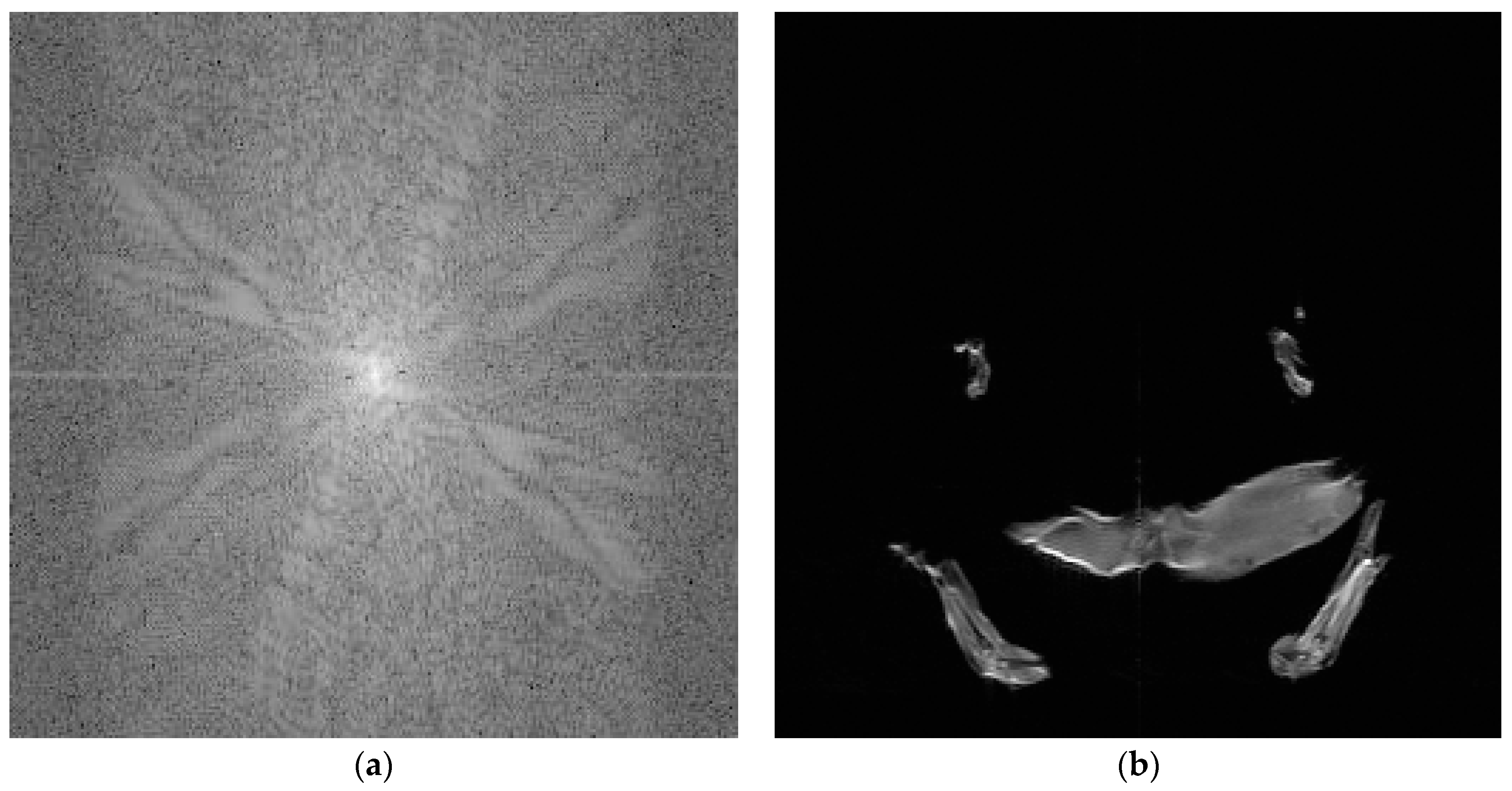
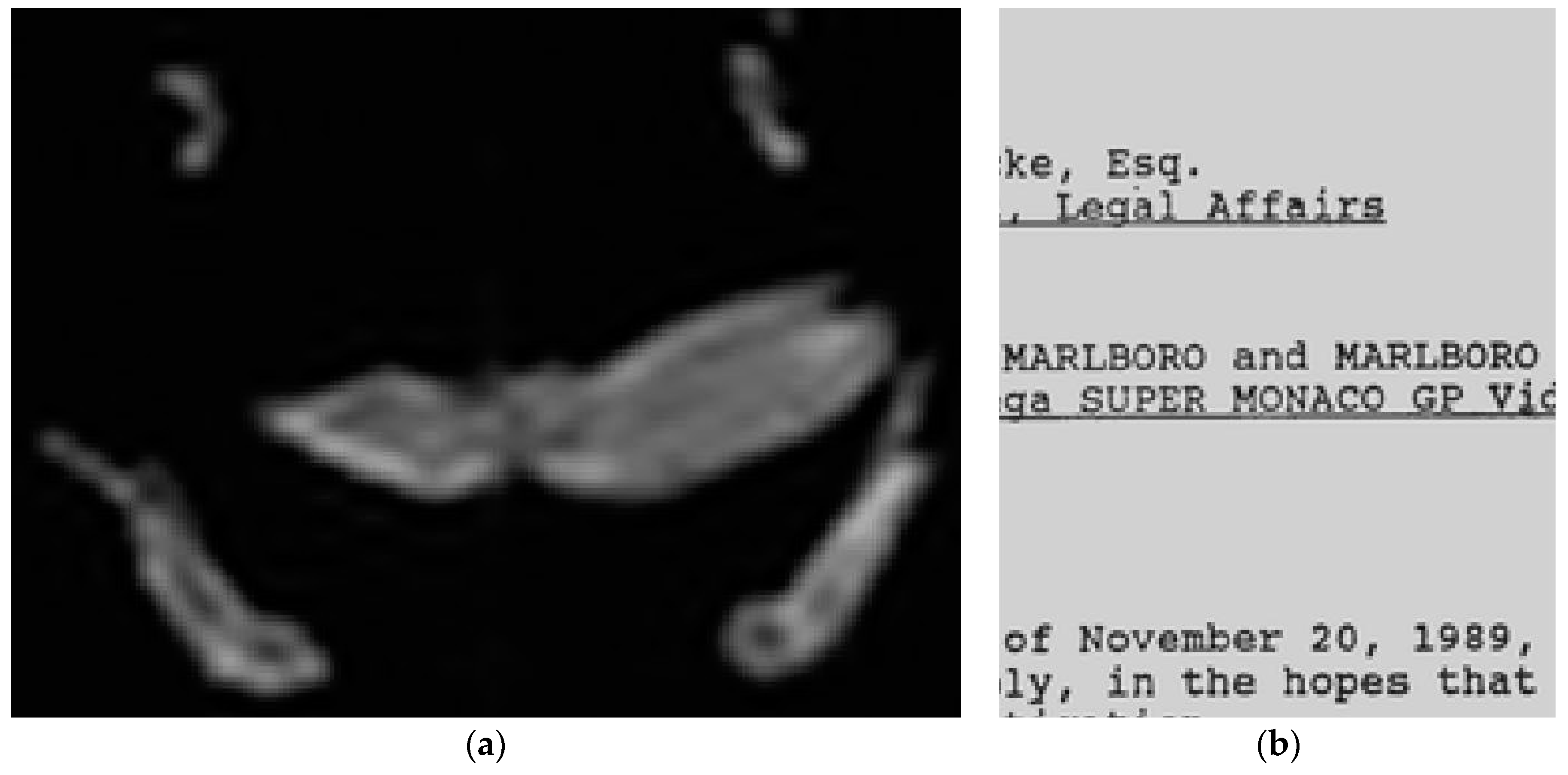
Experiment 3. From Experiments 1 and 2, we take the best decimator/interpolator pair and apply them on more samples. Our aim is to discover the intrinsic image properties that determine a certain behavior. As performed in the previous experiments, we also use a scale of four to compare the results. We run the tests on multiple images from the dataset described in Section 2 using a Hamming windowed sinc of size three as the decimator and a sine windowed sinc of 11 as an interpolator. Some representative results are analyzed in Figure 4 and Figure 5. As we can easily notice from the previously shown analysis in the frequency domain, the image yielding good results has a very low-frequency spectrum. As most of its energy is concentrated in the center of the spectrum, little to no information is lost when low-pass filtering it as a result of the interpolation process.
The image that produces bad interpolation results has a wider bandwidth and is thus more susceptible to losses of information due to the low pass filter applied. We give the results of the respective interpolant in both cases in
Figure 6.


