Article

Pm2.5 Time Series Imputation with Deep Learning and Interpolation

by
Anibal Flores
1,2,*,
Hugo Tito-Chura
1,2,
Deymor Centty-Villafuerte
3 and
Alejandro Ecos-Espino
4,5
1
Grupo de Investigación en Inteligencia Artificial, Universidad Nacional de Moquegua, Urb. Ciudad Jardin-Pacocha-Ilo, Moquegua 18611, Peru
2
Departamento Académico de Ingeniería de Sistemas e Informática, Universidad Nacional de Moquegua, Urb. Ciudad Jardin-Pacocha-Ilo, Moquegua 18611, Peru
3
Departamento de Ciencias Sociales y Humanidades, Universidad Nacional de Moquegua, Prolongación Calle Ancash S/N, Moquegua 18001, Peru
4
Departamento Académico de Ciencias Básicas, Universidad Nacional de Moquegua, Prolongación Calle Ancash S/N, Moquegua 18001, Peru
5
Instituto de Investigación para el Desarrollo del Perú (IINDEP), Universidad Nacional de Moquegua, Prolongación Calle Ancash S/N, Moquegua 18001, Peru
*
Author to whom correspondence should be addressed.
Computers 2023, 12(8), 165; https://doi.org/10.3390/computers12080165
Submission received: 18 July 2023 / Revised: 2 August 2023 / Accepted: 10 August 2023 / Published: 16 August 2023
(This article belongs to the Topic Artificial Intelligence Models, Tools and Applications)

Abstract

:
Commonly, regression for time series imputation has been implemented directly through regression models, statistical, machine learning, and deep learning techniques. In this work, a novel approach is proposed based on a classification model that determines the NA value class, and from this, two types of interpolations are implemented: polynomial or flipped polynomial. An hourly pm2.5 time series from Ilo City in southern Peru was chosen as a study case. The results obtained show that for gaps of one NA value, the proposal in most cases presents superior results to techniques such as ARIMA, LSTM, BiLSTM, GRU, and BiGRU; thus, on average, in terms of R2, the proposal exceeds implemented benchmark models by between 2.4341% and 19.96%. Finally, supported by the results, it can be stated that the proposal constitutes a good alternative for short-gaps imputation in pm2.5 time series.

1. Introduction

Time series forecasting is one of the most active research topics [1] in machine learning and deep learning; it is used in different domains such as biology, finance, meteorology, and social sciences [2], among others.
Missing values in time series is a common problem [2], and many machine and deep learning techniques do not work with missing data [3], so time series imputation becomes a very important task. It is also very important to mention that the quality of data for time series forecasting is very important [4], hence the importance of a good time series imputation process.
In this work, a novel approach for time series imputation is proposed, which combines a math technique with a deep learning one. The imputation problem is approached as a classification problem, and the proposal uses a classification model to determine the class of NA value, and from the class, an interpolation technique is implemented. The main motivation stems from the analysis of different short gaps of NA values in time series, where it was possible to identify two classes. The first, according to Figure 1a, comprises the NA values whose real values fit better to a polynomial interpolation. The second, according to Figure 1b, comprises the NA values whose real values fit better to a flipped polynomial interpolation. As can be seen in Figure 1, the NA value can be located above or below the line that joins the prior value (p0) with the next value (n0). Depending on the preceding values p1, p0 and following n0, n1, and derivatives, the NA value could be estimated more accurately with polynomial interpolation or flipped polynomial interpolation. The classification model was trained with 12 features, including the aforementioned p1, p0, n0, and n1, adding p2 and n2 and other derivatives of them that are described in detail in the Section 3 of this work.
The study case selected to validate the novel approach corresponds to hourly pm2.5 time series obtained from an environmental monitoring station in Ilo City in southern Peru. The study case was chosen due to the importance of the analysis of the pm2.5 time series since, as is known, long-term exposure to pm2.5 can cause diverse health issues, including heart disease [5], lung cancer [6], chronic obstructive pulmonary disease [7], lower respiratory infections (LRIs) [8], ischemic stroke [9], diabetes mellitus [10], and others. However, the pm2.5 time series presents NA values due to multiple factors such as equipment failure [11], power outages, etc., as occurs with the data from the monitoring station chosen. Therefore, the importance of implementing imputation techniques in order to recover lost data and made it available for the implementation of forecasting models.
The novel approach was compared with other state-of-the-art models for time series imputation, such as long short-term memory (LSTM) [12], bidirectional LSTM [13], gated recurrent unit (GRU) [14], bidirectional GRU, ARIMA, local average of nearest neighbors (LANN) [15], and polynomial interpolation.
The main contributions of this work are cited next:
-
A novel approach for pm2.5 time series imputation based on deep learning classification;
-
An ensemble deep learning model for NA values classification;
-
A comparative analysis between the proposal approach versus benchmark models.
The main limitations of this work are as follows: It is only focused on the analysis of short gaps, gives NA sequences of a single value in pm2.5 time series, and the interpolations are performed considering only four values: p1, p0, n0, and n1.
The rest of the paper is organized in Section 2 that briefly describes the work performed for pm2.5 time series imputation; Section 3, where the complete process for implementation of the proposal is described; and Section 4, where the achieved results are described and discussed according to the pros and cons of proposal results. The paper ends with Section 5.

2. Related Work

Some works for pm2.5 time series imputation where the use of machine learning and deep learning techniques were proposed are listed below in chronological order.
Xiao et al., 2018 [16] proposed an ensemble model for pm2.5 time series imputation. The proposal presents superior results to models such as random forest (RF), extreme gradient boosting (XGBoosting), and the generalized additive model (GAM). Yuan et al., 2018 [17] proposed the RNN long short-term memory (LSTM) for the imputation process and compared this technique with two classic techniques: moving average and mean imputation. The results show the enormous superiority of LSTM over the other two techniques.
Belachsen et al., 2022 [18] proposed a multivariate KNN technique for half-hourly pm2.5 time series reaching an NMAE between 0.21 and 0.26. Saif-ul-Allah et al., 2022 [19] proposed the recurrent neural network known as GRU, reaching an RMSE of 10.60 ug/m3 and surpassing other models such as SVM, LSTM, and BiLSTM. Alkabbani et al., 2022 [20] proposed a multivariate random forest model for pm2.5 time series imputation, and the results were compared only with linear interpolation, showing that random forest achieves the best RMSE (3.756 ug/m3).
Yldz et al., 2022 [21] proposed a transformer model for multivariate time series imputation; they experimented with air quality (pm2.5) and healthcare time series. For pm2.5, they worked with hourly data of 12 months, obtaining a MAE = 8.31 ug/m3 that exceeded those obtained by benchmark models such as BRITS, RDIS, V-RIN, etc.
Lee et al., 2023 [22] proposed four machine learning models, namely GAIN, FCDNN, random forest, and KNN, and the best results were obtained with the GAIN model with R2 = 0.895.
Reviewing other related works for time series imputation, in general, it can be noted that these address techniques ranging from moving averages: simple moving average (SMA), linear weighted moving average (LWMA), exponential weighted moving average (EWMA), and interpolation techniques (linear, spline, and Stinneman), all generally implemented in the imputeTS library [2,18] of R. On the other hand, there were also deep learning-based ones, including LSTM [23,24], GRU [25], and GAN [26] and some variants such as BRITS [27], GRU-D [28], and B-CIPIT [29].
The main difference between the related works and the proposal is that these works to estimate NA values generally apply a regression model in some cases associated with a time series transformation. In our model, at the beginning, NA features were extracted and labeled; then, features were normalized; next, a time series classification task with deep learning models was performed, followed by the implementation of an ensemble model; finally the class of an NA value was estimated, and from this, the proper polynomial interpolation was performed to obtain the estimated NA value. Figure 2 summarizes this process.

3. Materials and Methods

The methodology used for the implementation of proposal approach is summarized in Figure 3.

3.1. Data Preparation

The hourly data used for this work were downloaded from OEFA’s server located at http://fiscamb.oefa.gob.pe/vig_amb/ accessed on 2 May 2023, and they oscillate between 1 August 2020 and 30 April 2023, corresponding to the Pacocha environmental monitoring station located at Ilo Province and Pacocha District in southern Peru. The downloaded data present several missing values, so the days that presented some missing values were discarded. After this process, the total available records numbered 56,424. As it is a regression problem, the dataset was just split into two sets (training and test) [30]. For training, 48,792 records were used (80%), and 7632 records were used for testing (20%). Figure 4 shows a sample of 1000 h of the selected time series. Data normalization was performed for extracted features during the implementation of classification models; it is described in Section 3.2.3.

3.2. Implementation of Classification Models

For classification models, the dataset was split into three sets: training, validation, and test. For the proposal, from 48,792 records corresponding to the training data, 70% was used for training, 10% for validation, and the remaining 20% was used for testing the classification models.
Therefore, at this stage, the first task we performed corresponds to feature extraction and labeling of NA values, which is described below.

3.2.1. Feature Extraction and Labelling

The features that were extracted from the time series are described in Table 1.
The motivation to use the described features for NA values classification was the method by which moving averages techniques work: they use a parameter k that corresponds to the window size. The window size tells the technique how many values before and after the NA value should be used for the corresponding estimation; thus, p2, p1, p0, n0, n1, and n2 were obtained considering a window size k = 3. For future work, higher values could be used. The rest of the features were derived or synthetic; that is, they were generated to provide more information for model training.
Given a t time series, the features shown in Table 1 were extracted using the algorithm shown in Figure 5.
The algorithm shown in Figure 5 received as an argument a time series t, which was traversed from beginning to end. As can be seen, the feature extraction was quite simple: p2, p1, p0, n0, n2, and n2 were estimated from the position of the NA value; mid, mid1, and mid2 are averages of p1, p0, n0, and n1; diff, slope1, and slope2 are the differences between p1, p0, n0, and n1. However, the estimation of the class or label is somewhat complex, and it requires that certain conditions be met; these conditions are detailed in Table 2.

3.2.2. Feature Selection

For this task, a correlation matrix was implemented, which can be seen in Figure 6.
According to the last row or last column of the correlation matrix, the relationship between the input features and the target feature was not strong; thus, it would not be easy to obtain good results in terms of accuracy, precision, recall, and f1-score. In this work, it was decided to use all the input features for classification models.

3.2.3. Normalization

Before the implementation of deep learning models, normalization is very important in order to ensure their faster convergence. In this study, z-score normalization was used; it can be implemented through Equation (1).
X = x x σ
where
  • x : normalized vector;
  • x : original feature vector;
  • x : mean of the feature vector;
  • σ : standard deviation of the feature vector.

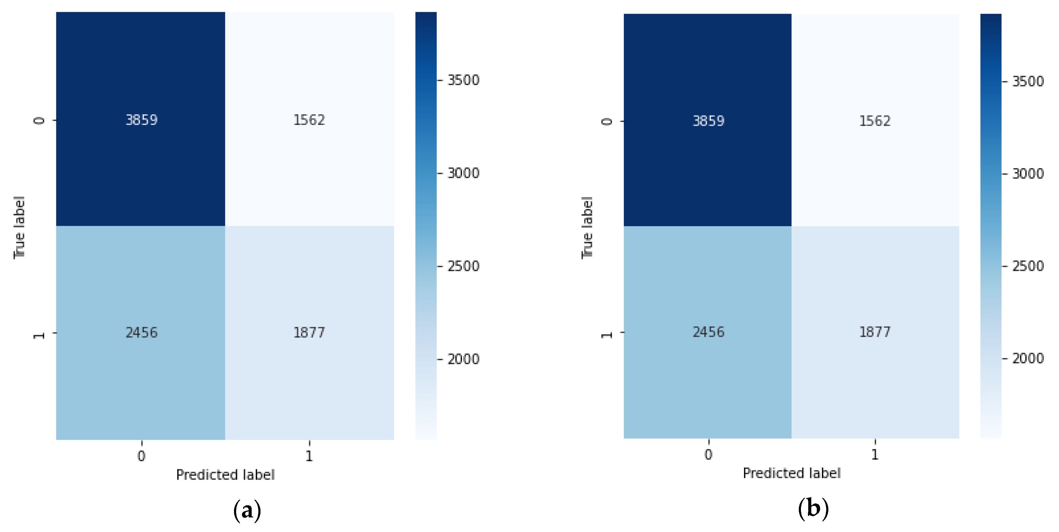
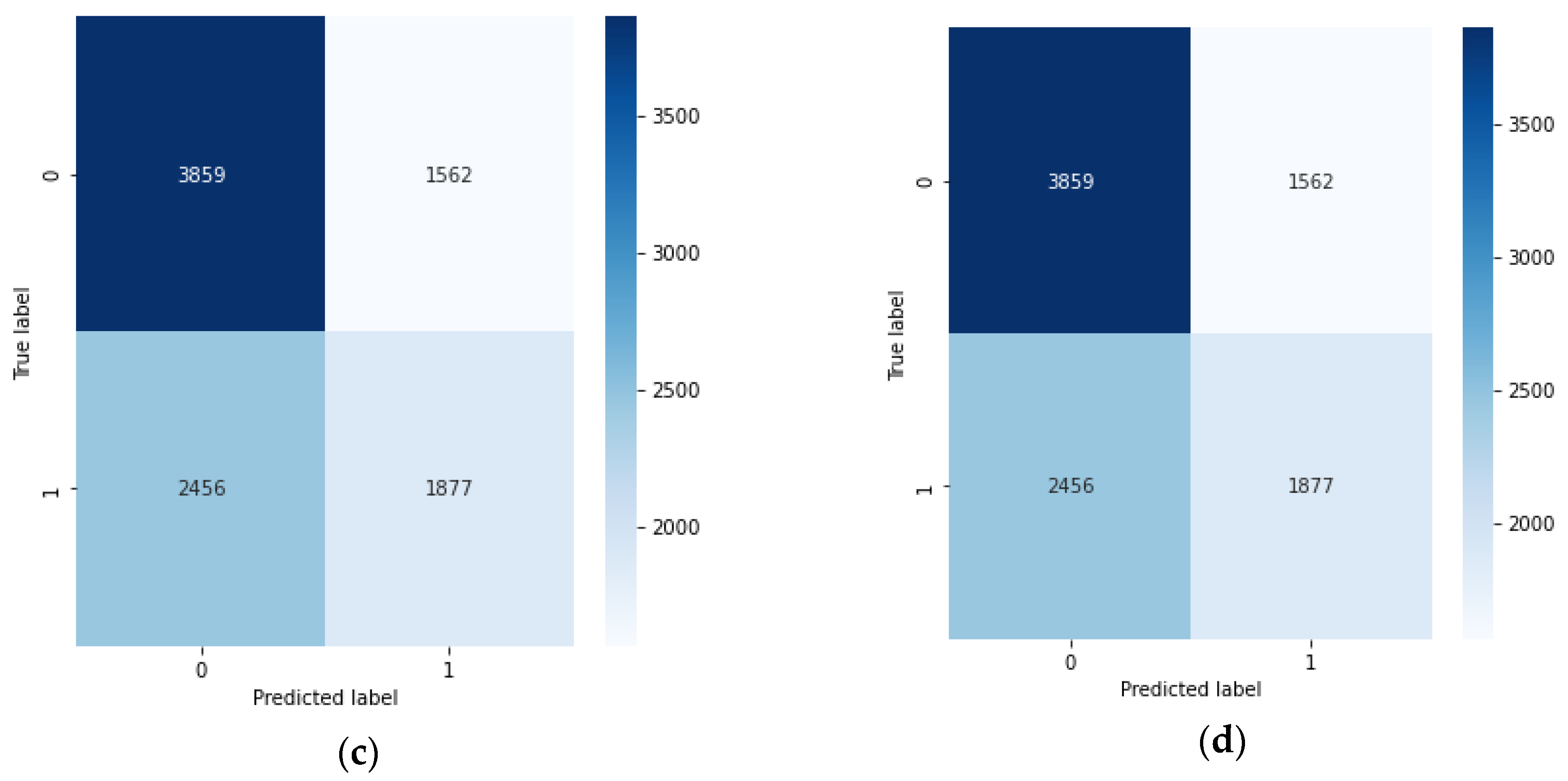
3.2.4. Deep Learning Classification Models

In this stage, four deep learning models were implemented, including deep neural networks (DNN), convolutional neural networks (DNN), long short-term memory (LSTM), and gated recurrent unit (GRU), whose architectures are described in Table 3.
According to Table 3, all classification models use a learning rate of 0.0001 and dropout rates of 0.1 after all layers except the output layer. The DNN presents an architecture with a greater number of layers than the other models, all with relu as the activation function with 10 neurons in the input layer; 20, 40, and 10 in the hidden layers; and 1 neuron in the output layer with sigmoid the as activation function. Regarding the CNN model, it presents its first two Conv1-type layers with relu as activation function, followed by a MaxPooling1D layer with pool_size = 2, then a dense layer of 10 neurons, and, finally, a dense layer with 1 neuron. The LSTM and GRU RNNs present identical architectures: one input layer with 30 neurons, two hidden layers with 30 neurons each, and an output layer of 1 neuron.
All models were compiled with Adam as optimizer, loss function: binary_crossentropy, 200 epochs, and batch_size = 1000. Jupyter and Tensorflow 2.9.0 were used.

3.2.5. Evaluation

The results of the classification models based on deep learning are shown in Table 4. These are described in terms of accuracy (2), precision (3), recall (4), and f1-score (5).
A c c u r a c y = T P + T N T P + F P + T N + F N
P r e c i s i o n = T P T P + F P
R e c a l l = T P T P + F N
f 1 s c o r e = 2 P r e c i s i o n R e c a l l ( P r e c i s i o n + R e c a l l )
Once the classification models were compiled, they were evaluated in test data. The respective confusion matrices are shown in Figure 7.
From the confusion matrices and Equations (2) and (5)–(7), the metrics shown in Table 4 were estimated.
According to Table 4 and Figure 7, it can be seen that the results of the classification models are not good, and it can be seen that the main difficulty presented by the implemented models is the low capacity to detect true positives (NAs of class 1); this is reflected in the recall below 43% and f1-score below 48%.
In order to improve the results, the strategy of implementing an ensemble model based on average was used. For this, it was experimented by assembling all the models and combinations of three models. Figure 8 shows the respective ROC curves, and as it can be seen, the ensemble model based on DNN, CNN, and LSTM presented the best area under the curve (AUC of 0.611), which is why this ensemble model was chosen for the imputation process. In terms of accuracy, recall, precision, and f1-score, the ensemble model reached 0.5859, 0.4045, 0.5457, and 0.4647, respectively.

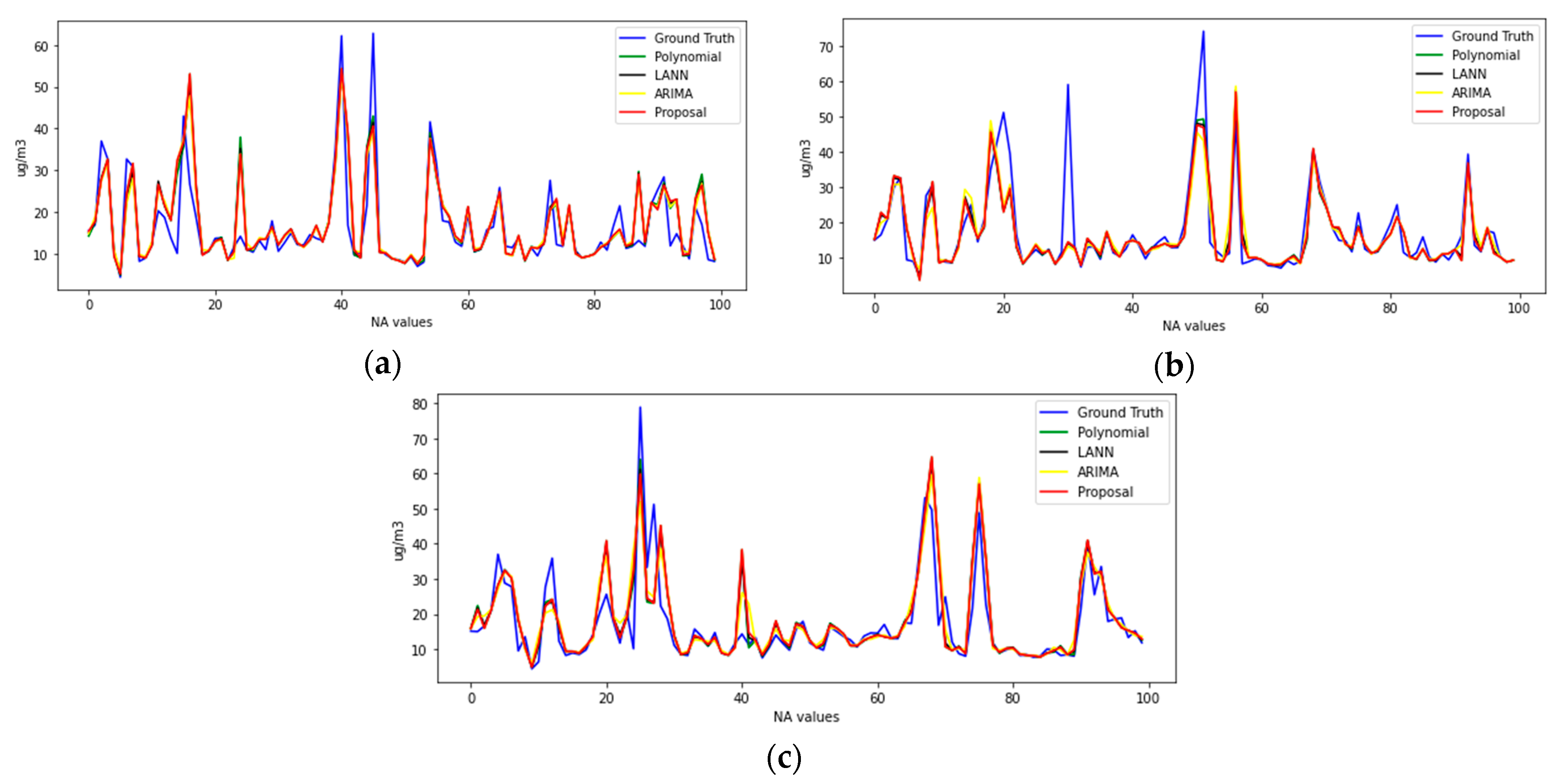
3.3. Imputation of NA Values

Once the classification model for NA class estimation was obtained, the pm2.5 time series imputation process using the proposal was as described below.

3.3.1. Generation of NA Values in Test Data

NA values were generated considering gaps of a single NA value. Three different sets of NA values were implemented: 19.98% (1525 items), 25.00% (1907 items), and 33.32% (2543 items).
The NA values insertion mechanism was quite simple: to achieve 19.98% of NA values, one NA value was inserted into the test data every four items. To achieve 25.00%, NA values were inserted every three items, and to achieve 33.32%, NA values were inserted every two items. In this way, for each set, it was possible to obtain different amounts and configurations for the NA values. The partial result of this process can be visualized in Figure 9.

3.3.2. Class Estimation for NA Values

To estimate the class of each NA value in every NA set, a Python function was created.
The .h5 files correspond to DNN, CNN, and LSTM models that are part of the selected ensemble model to estimate the classes of NA values. The Python function getClass receives as the input parameter the characteristics of all NA values to be estimated, and then, it returns the classes to which they correspond. Figure 10 shows such a function.

3.3.3. Interpolation according to Class Estimation

For polynomial interpolation, the first step is to determine the coefficients of the polynomial function; for this, there are various techniques, including the Lagrange method, which is described below.
Given the n points (x0, y0), …, (xn1, yn1), the Lagrange polynomial is estimated through Equation (6).
p x = i = 0 n 1 y i j i ( x x j ) j i ( x i x j )
From (6), the coefficients are obtained, and the polynomial function can be implemented, and from it, any point can be estimated, in this case, the point corresponding to the NA value. The polynomial function is similar to what is shown in Equation (7).
p x = a 0 + a 1 x + a 2 x 2 + + a n 1 x n 1
The algorithm that implements the interpolations according to the estimated class is shown in Figure 11.
According to Figure 10, the getNA procedure for NA estimation receives as parameters the NA class and the vector y that contains the four values to be used by polynomial interpolation: p1, p0, n0, and n1. The p0 and n0 are interpolated, and mid is obtained; then, the coefficients of the polynomial function are obtained for the four values in y, and for this, a polynomial procedure is used (See Figure 12). With the polynomial obtained, the value in position 1.5 is estimated, which corresponds to the NA value according to Figure 1; for this, the procedure interpolate is used (see Figure 13), and for na, this is the final result for NA values of class 0. For the case of NA values of class 1, the na value is flipped; for this, the absolute distance d between the na value and mid is determined, and depending on the location of the na value according to mid, d is subtracted or added.
The polynomial procedure receives as parameters the number of points (points) and the vectors of values in x (Xs) and y (Ys). With these data, according to Equation (6), for each point, Equation (8) is estimated, and from this, Equation (9) must be estimated.
t e m p = y i j i ( x i x j )
t e r m = t e m p ( j i ( x x j ) )
Between lines 9 and 19 of the algorithm, Equation (8) is estimated, and Equation (9) is estimated between lines 20 and 29. The last part of the algorithm generates the coefficients of the polynomial function.
The interpolate procedure algorithm receives as parameters the coefficients of the polynomial (poly) and the position of the value to be estimated (v = x = 1.5), which in this case corresponds to the position of the NA value, and from this, Equation (7) is implemented.
The source code of the proposal can be downloaded from the next link: https://drive.google.com/drive/folders/1qL-k80rXqjFVmi-4fubg6nFvQbj3-Xq6?usp=drive_link accessed on 2 August 2023.

3.4. Implementation of Benchmark Models
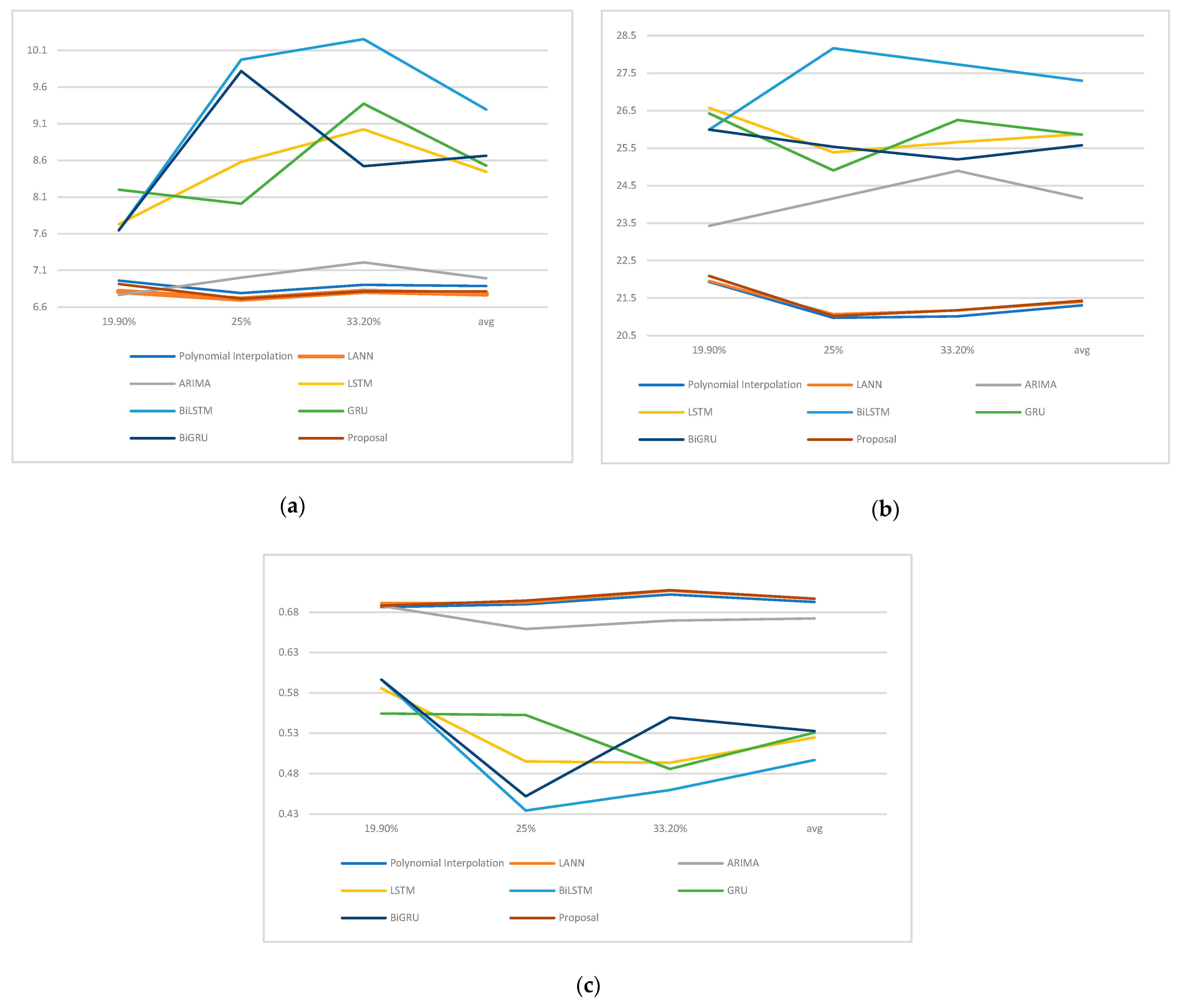
Seven benchmark models were implemented in order to compare the proposal performance; these models include polynomial interpolation, LANN, ARIMA, long short-term memory (LSTM), bidirectional LSTM, gated recurrent unit (GRU), and bidirectional GRU.
Polynomial interpolation and ARIMA were implemented in R language using the imputeTS library. For ARIMA, the auto.arima model was used.
Deep regression models were implemented in Python using tensorflow 2.9.0, and the hyperparameters can be seen in Table 5.
All deep regression models use Adam as the optimizer, mean standard error (mse) as the loss function, and 0.001 as learning rate. Also, the number of epochs used was 100, and the batch_size was 100, too. Finally, all layers used relu as the activation function except the output one-neuron layer, which used sigmoid as the activation function.

3.5. Evaluation

The proposal is evaluated in terms of root mean squared error (RMSE), mean absolute percentage error (MAPE), and R2, which are implemented through Equations (10)–(12)
R M S E = i = 1 n P i O i 2 n
M A P E = 1 n i = 1 n O i P i O i 100
R 2 = 1 ( i = 1 n O i P i 2 / i = 1 n O i O 2 )
where
  • n: Number of observed/predicted values;
  • Pi: Vector of predicted values;
  • Oi: Vector of observed values;
  • O : Mean of observed values.

4. Results and Discussion

This section describes the results achieved by the proposal, comparing them with other models in the literature.

4.1. Results

The results achieved by the proposal are described below; likewise, these are compared with other techniques and models of the literature and the state of the art.
According to Table 6 and Figure 14a, it can be seen that, in terms of RMSE, the lowest error was reached by the proposal in one of the three NA sets; it was the best in the third NA set (33.32%) with 6.8134 ug/m3. For the first NA set (19.98%), the best technique was ARIMA with RMSE = 6.7654 ug/m3, followed by LANN with RMSE = 6.8123 ug/m3, and with the proposal with RMSE = 6.9148 ug/m3 in third place. For the second NA set (25.00%), the best technique was LANN with RMSE = 6.7088 ug/m3, followed by the proposal with RMSE = 6.7137 ug/m3, and with polynomial interpolation in third place with RMSE = 6.7912 ug/m3.
In terms of MAPE, according to Table 7 and Figure 14b, in all sets of NAs, the polynomial interpolation model presented the best results, surpassing all implemented models, including the proposal. For the first NA set (19.98%), LANN was in second place with MAPE = 21.9548, and the proposal was in third place with MAPE = 22.0901. For the second NA set, (25.00%), the proposal was in second place with MAPE = 21.0242%, and in third place was LANN with MAPE = 21.0718. For the third NA set (33.32%), LANN was in second place with MAPE = 21.1710, followed by the proposal with MAPE = 21.1758.
In terms of R2, according to Table 8 and Figure 14c, the proposal model outperformed all benchmark models in two of three NA sets. In the first NA set (19.98%), LANN was the best with R2 = 0.6911, followed by the proposal and polynomial interpolation with 0.6879 and 0.6861, respectively. In the second NA set (25.00%), the proposal was the best with R2 = 0.6941, followed by LANN and polynomial interpolation with 0.6916 and 0.6859, respectively. Finally, in the third NA set, the proposal was also the best with R2 = 0.7072, followed by LANN and polynomial interpolation with 0.7062 and 0.7018, respectively.
On average, according to the above, there is a notable difference between the proposal and the benchmarks models based on deep learning, such as LSTM, BiLSTM, GRU, and BiGRU; in terms of RMSE, the difference is between 1.6298 ug/m3 and 2.4773 ug/m3; in terms of MAPE, it is between 4.1459% and 5.8669%; and in terms of R2, it is between 16.3818% and 19.9618%.
However, comparing the proposal with benchmark models such as LANN, polynomial interpolation, and ARIMA, the difference is smaller. On average, in terms of RMSE, LANN alone is better than the proposal by a small 0.03527 ug/m3. In terms of MAPE, only polynomial interpolation and LANN are better than the proposal by 0.1239% and 0.0309%, respectively. In terms of R2, the proposal is better than polynomial interpolation, LANN, and ARIMA by 0.3898%, 0.0134%, and 2.4341%, respectively.
Graphically, Figure 15 shows the results of the best benchmark models and the proposal for the first 100 items of ground truth for the different sets of NAs.

4.2. Discussions

Through analysis of the results, it can be seen that the closer models to the proposal model are LANN and polynomial interpolation. Polynomial interpolation served as the basis for the proposal, as it was used to estimate the NA values of class 0. In the proposal, thanks to the implementation of the flipped polynomial interpolation for NA class 1, the proposal outperformed the polynomial interpolation benchmark on average by 0.0712 ug/m3 and 0.3898% in terms of RMSE and R2, respectively.
The good results obtained in the estimation of NA values even though the classification models did not achieve good performances, according to Figure 1, prove that both interpolations have similar estimates, so the class estimation errors do not affect them greatly.
Despite what is mentioned in the preceding paragraph, the main weakness of the proposal is the complexity of the classification task to estimate the NA class since it was not possible to identify good input features that have a higher correlation with the target feature. The classification models in most of the evaluation metrics present values below 60%; this can be improved by using a larger amount of data for the training phase and generating or obtaining better input features. A better classification rate would make it possible to identify the NA classes with greater accuracy and, from this, obtain better NA value estimations, reducing the RMSE and MAPE and increasing the R2 coefficient.
Another aspect that should be analyzed for future work lies in the distance between the real NA value and the value that can be estimated by polynomial interpolation. If the real NA value is further from the polynomial curve, the estimation error will be larger. This constitutes a limitation of this type of technique to estimate more complex values. This type of technique is good for NA values that are close to the line between p0 and n0. For this reason, LANN produces good results, too.
Also, even though in most cases the proposal presented higher R2s than the benchmark ones, the R2 coefficient has to be improved, as in two of three NA sets, the proposal presented a value below 0.7, and just in one set, it presented an R2 above 0.7. As was mentioned in the previous case, improving the classification rate will improve the R2 of the proposal, too.
On the other hand, considering that related works used other datasets, and each dataset presents different characteristics, the comparison is carried out only for reference. According to Table 9, it can be seen that in terms of RMSE, the proposal is only below the work [20], which obtained an RMSE of 3.756 ug/m3; in terms of R2, the proposal with R2 of 0.6946 is below the work [22], which reported an R2 of 0.895; and in terms of MAE, the proposal with MAE = 3.4944 ug/m3 exceeded the work [21] with MAE = 8.31 ug/m3.

5. Conclusions and Future Work

5.1. Conclusions

Although the classification rate of the types or classes of NA values did not exceed 60% in most of the analyzed metrics, the estimation results of NA values obtained in terms of RMSE, MAPE, and R2 are very promising because when compared with the results of benchmark models, the proposal managed to widely outperform the state-of-the-art models, such as LSTM, BiLSTM, GRU, BiGRU and ARIMA, demonstrating that for short gaps, the proposal is a good alternative.

5.2. Future Work

As previously mentioned, this work experimented only with short gaps—gaps of one NA value. For future work, it would be important to adapt the proposal for gaps of more than one value. Likewise, as mentioned above, the classification models only reached accuracies, recalls, precisions, and f1-scores below 60%, which indicates that there is still a wide margin for improvement; in this sense, other architectures of deep learning could be implemented, offering a greater number of layers and different configurations of neurons, among others. Also, the dataset could be enriched through data augmentation techniques for time series classification in order to generate a greater diversity of rows that could help to improve the performance of the models. Also, LANN could be exploited through the creation of a new class (2), which could contain the NA values that can be estimated with greater accuracy with linear interpolation instead of polynomial interpolation.
On the other hand, fractal theory could help to find other time series features that could improve the time series classification process. Likewise, the proposal approach of this work can also be adapted for time series of similar contexts, such as pm10, SO2, etc., and other different ones like meteorology, biology, finance, etc.

Author Contributions

Conceptualization, A.F., H.T.-C. and D.C.-V.; methodology, A.F.; software, A.F.; validation, A.F., H.T.-C. and A.E.-E.; formal analysis, A.E.-E.; investigation, A.F.; resources, D.C.-V.; data curation, A.F. and H.T.-C.; writing—original draft preparation, A.F.; writing—review and editing, H.T.-C. and D.C.-V.; visualization, A.F.; supervision, A.E.-E.; project administration, H.T.-C.; funding acquisition, A.E.-E. All authors have read and agreed to the published version of the manuscript.

Funding

This research received no external funding and the APC was funded by Universidad Nacional de Moquegua.

Data Availability Statement

Data are available at “http://fiscamb.oefa.gob.pe/vig_amb/ (accessed on 2 May 2023)” or by contact to the corresponding author.

Conflicts of Interest

The authors declare no conflict of interest.

References

  1. Spadon, G.; Hong, S.; Brandoli, B.; Matwin, S.; Rodrigues, J.F., Jr.; Sun, J. Pay Attention to Evolution: Time Series Forecasting with Deep Graph-Evolution Learning. IEEE Trans. Pattern Anal. Mach. Intell. 2021, 44, 5368–5384. [Google Scholar] [CrossRef] [PubMed]
  2. Moritz, S.; Bartz-Beielstein, T. imputeTS: Time series missing value imputation in R. R J. 2017, 9, 207–218. [Google Scholar] [CrossRef]
  3. Peker, N.; Kubat, C. A Hybrid modified deep learning data imputation method for numeric datasets. Int. J. Intell. Syst. Appl. Eng. 2021, 9, 6–11. [Google Scholar] [CrossRef]
  4. Chen, C.; Xue, X. A novel coupling preprocessing approach for handling missing data in water quality prediction. J. Hydrol. 2023, 617, 128901. [Google Scholar] [CrossRef]
  5. Oh, J.; Choi, S.; Han, C.; Lee, D.-W.; Ha, E.; Kim, S.; Bae, H.-J.; Pyun, W.B.; Hong, Y.-C.; Lim, Y.-H. Association of long-term exposure to PM2.5 and survival following ischemic heart disease. Environ. Res. 2023, 216, 114440. [Google Scholar] [CrossRef] [PubMed]
  6. Huang, F.; Pan, B.; Wu, J.; Chen, E.; Chen, L. Relationship between exposure to PM2.5 and lung cancer incidence and mortality: A meta-analysis. Oncotarget 2017, 8, 43322–43331. [Google Scholar] [CrossRef] [PubMed]
  7. Su, J.; Ye, Q.; Zhang, D.; Zhou, J.; Tao, R.; Ding, Z.; Lu, G.; Liu, J.; Xu, F. Joint association of cigarette smoking and PM2.5 with COPD among urban and rural adults in regional China. BMC Pulm. Med. 2021, 21, 87. [Google Scholar] [CrossRef]
  8. Bu, X.; Xie, Z.; Liu, J.; Wei, L.; Wang, X.; Chen, M.; Ren, H. Global PM2.5-attributable health burden from 1990 to 2017: Estimates from the Global Burden of disease study 2017. Environ. Res. 2021, 197, 111123. [Google Scholar] [CrossRef]
  9. Chen, Z.; Liu, P.; Xia, X.; Wang, L.; Li, X. The underlying mechanism of PM2.5-induced ischemic stroke. Environ. Pollut. 2022, 310, 119827. [Google Scholar] [CrossRef]
  10. Lee, M.; Ohde, S. PM2.5 and diabetes in the Japanese population. Int. J. Environ. Res. Public Health 2021, 18, 6653. [Google Scholar] [CrossRef]
  11. Liu, Q.; Liu, W.; Mei, J.; Si, G.; Xia, T.; Quan, J. A New Support Vector Regression Model for Equipment Health Diagnosis with Small Sample Data Missing and Its Application. Shock. Vib. 2021, 2021, 6675078. [Google Scholar] [CrossRef]
  12. Hochreiter, S.; Schmidhuber, J. Long Short-Term Memory. Neural Comput. 1997, 9, 1735–1780. [Google Scholar] [CrossRef] [PubMed]
  13. Graves, A.; Fernández, S.; Schmidhuber, J. Bidirectional LSTM networks for improved phoneme classification and recognition. In Proceedings of the International Conference on Artificial Neural Networks, Warsaw, Poland, 11–15 September 2005; Lecture Notes in Computer Science; Springer Science and Business Media LLC: Berlin/Heidelberg, Germany, 2005; pp. 799–804. [Google Scholar] [CrossRef]
  14. Chung, J.; Gulcehre, C.; Cho, K.; Bengio, Y. Gated Recurrent Neural Networks on Sequence Modeling. arXiv 2014, arXiv:1412.3555. [Google Scholar]
  15. Flores, A.; Tito, H.; Silva, C. Local average of nearest neighbors: Univariate time series imputation. Int. J. Adv. Comput. Sci. Appl. 2019, 10, 45–50. [Google Scholar] [CrossRef]
  16. Xiao, Q.; Chang, H.H.; Geng, G.; Liu, Y. An Ensemble Machine-Learning Model To Predict Historical PM2.5 Concentrations in China from Satellite Data. Environ. Sci. Technol. 2018, 52, 13260–13269. [Google Scholar] [CrossRef]
  17. Yuan, H.; Xu, G.; Yao, Z.; Jia, J.; Zhang, Y. Imputation of missing data in time series for air pollutants using long short-term memory recurrent neural networks. In Proceedings of the 2018 ACM International Joint Conference on Pervasive and Ubiquitous Computing, Singapore, 8–12 October 2018; pp. 1293–1300. [Google Scholar] [CrossRef]
  18. Belachsen, I.; Broday, D.M. Imputation of Missing PM2.5 Observations in a Network of Air Quality Monitoring Stations by a New kNN Method. Atmosphere 2022, 13, 1934. [Google Scholar] [CrossRef]
  19. Saif-Ul-Allah, M.W.; Qyyum, M.A.; Ul-Haq, N.; Salman, C.A.; Ahmed, F. Gated Recurrent Unit Coupled with Projection to Model Plane Imputation for the PM2.5 Prediction for Guangzhou City, China. Front. Environ. Sci. 2022, 9, 816616. [Google Scholar] [CrossRef]
  20. Alkabbani, H.; Ramadan, A.; Zhu, Q.; Elkamel, A. An Improved Air Quality Index Machine Learning-Based Forecasting with Multivariate Data Imputation Approach. Atmosphere 2022, 13, 1144. [Google Scholar] [CrossRef]
  21. Yldz, A.Y.; Koc, E.; Koc, A. Multivariate Time Series Imputation with Transformers. IEEE Signal Process. Lett. 2022, 29, 2517–2521. [Google Scholar] [CrossRef]
  22. Lee, Y.S.; Choi, E.; Park, M.; Jo, H.; Park, M.; Nam, E.; Kim, D.G.; Yi, S.-M.; Kim, J.Y. Feature extraction and prediction of fine particulate matter (PM2.5) chemical constituents using four machine learning models. Expert Syst. Appl. 2023, 221, 119696. [Google Scholar] [CrossRef]
  23. Yang, J.; Lai, X.; Zhang, L. Auto-Associative LSTM for Multivariate Time Series Imputation. In Proceedings of the 2022 41st Chinese Control Conference (CCC), Hefei, China, 25–27 July 2022. [Google Scholar] [CrossRef]
  24. Li, D.; Li, L.; Li, X.; Ke, Z.; Hu, Q. Smoothed LSTM-AE: A spatio-temporal deep model for multiple time-series missing imputation. Neurocomputing 2020, 411, 351–363. [Google Scholar] [CrossRef]
  25. Zaman, M.A.U.; Du, D. A Stochastic Multivariate Irregularly Sampled Time Series Imputation Method for Electronic Health Records. Biomedinformatics 2021, 1, 166–181. [Google Scholar] [CrossRef]
  26. Zhang, W.; Luo, Y.; Zhang, Y.; Srinivasan, D. SolarGAN: Multivariate solar data imputation using generative adversarial network. IEEE Trans. Sustain. Energy 2020, 12, 743–746. [Google Scholar] [CrossRef]
  27. Cao, W.; Zhou, H.; Wang, D.; Li, Y.; Li, J.; Li, L. BRITS: Bidirectional recurrent imputation for time series. In Proceedings of the Advances in Neural Information Processing Systems 31 (NeurIPS 2018), Montréal, QC, Canada, 3–8 December 2018. [Google Scholar]
  28. Che, Z.; Purushotham, S.; Cho, K.; Sontag, D.; Liu, Y. Recurrent Neural Networks for Multivariate Time Series with Missing Values. Sci. Rep. 2018, 8, 6085. [Google Scholar] [CrossRef]
  29. Guo, Y.; Poh, J.W.J.; Wong, C.S.Y.; Ramasamy, S. Bayesian Continual Imputation and Prediction For Irregularly Sampled Time Series Data. In Proceedings of the ICASSP 2011—IEEE International Conference on Acoustics, Speech and Signal Processing, Singapore, 23–27 May 2022; pp. 4493–4497. [Google Scholar] [CrossRef]
  30. Brownlee, J. Ensemble Learning Algorithms with Python. Machine Learning Mastery. 2021. [Google Scholar]
Figure 1. Types of NA values. (a) Class 0 and (b) class 1.
Computers 12 00165 g001
Figure 2. Comparison between literature approaches and proposal approach.
Computers 12 00165 g002
Figure 3. Methodology for the implementation of proposal approach.
Computers 12 00165 g003
Figure 4. Sample of 1000 h of pm2.5 time series.
Computers 12 00165 g004
Figure 5. Feature extraction algorithm of NA values.
Computers 12 00165 g005
Figure 6. Correlation matrix.
Computers 12 00165 g006
Figure 7. Confusion matrices of implemented classification models. (a) DNN, (b) CNN, (c) LSTM, and (d) GRU.
Computers 12 00165 g007aComputers 12 00165 g007b
Figure 8. ROC curves of implemented and ensemble models.
Computers 12 00165 g008
Figure 9. Sets of NA values in test data.
Computers 12 00165 g009
Figure 10. Procedure for Classes Estimation of NA values.
Computers 12 00165 g010
Figure 11. Algorithm for NA estimation.
Computers 12 00165 g011
Figure 12. Algorithm of polynomial procedure.
Computers 12 00165 g012
Figure 13. Algorithm of interpolate procedure.
Computers 12 00165 g013
Figure 14. Metrics of implemented models. (a) RMSE, (b) MAPE, and (c) R2.
Computers 12 00165 g014
Figure 15. First 100 predicted values: proposal vs. best benchmark models (polynomial interpolation, LANN, and ARIMA). (a) NA set 19.98%, (b) NA set 25.00%, and (c) NA set 33.32%.
Computers 12 00165 g015
Table 1. Features for NA values.
FeatureDescription
p0Prior value to NA
p1Before p0
p2Before p1
n0Next value of NA
n1After n0
n2After n1
midMean between prior (p0) and next value (n0)
mid1Mean between prior values (p1) and next value (p0)
mid2Mean between next values (n0) and next value (n1)
diffDifference between prior and next values
slope1Slope between p1 and p0
slope2Slope between n0 and n1
labelClass of NA value.
0, corresponding to polynomial interpolation
1, corresponding to flipped polynomial interpolation.
Table 2. Conditions for NA classes.
ClassConditions
0 (polynomial interpolation)According to Figure 1a, the conditions to apply polynomial interpolation are two cases:
Case 1: When na is below the line (p0 to n0), it can be stated through the next conditions:
   na ≤ mid
   p1 ≥ p0
Case 2: When na is above the line (p0 to n0). The two conditions to be met are:
   na > mid
   p0 > p1
1 (flipped polynomial interpolation)According to Figure 1b, the conditions to apply flipped polynomial interpolation are two:
Case 1: When na is below the line (p0 to n0), it can be stated through the next conditions:
   na < mid
   p1 < p0
Case 2: When na is above the line (p0 to n0). The two conditions to be met are:
   na > mid
   p0 ≤ p1
Table 3. Architectures of deep learning classification models.
ModelHyperparameters
DNN(0, 20, 40, 10, 1), learning_rate: 0.0001, dropout_rate (0.1)
CNN(20, 50, 10, 1), learning_rate: 0.0001, dropout_rate (0.1)
LSTM(30, 30, 30, 1), learning_rate: 0.0001, dropout_rate (0.1)
GRU(30, 30, 30, 1), learning_rate: 0.0001, dropout_rate (0.1)
Table 4. Results of deep learning classification models.
ModelAccuracyRecallPrecisionF1-Score
DNN0.59720.30830.58910.4048
CNN0.59120.42230.55220.4786
LSTM0.58590.36440.55130.4388
GRU0.58590.40460.54580.4647
Table 5. Hyperparameters for deep regression models.
ModelHyperparameters
LSTMarchitecture: [40, 30, 30, 40, 1], dropout_rate: 0.2
BiLSTMarchitecture: [30, 30, 30, 1], dropout_rate: 0.1
GRUarchitecture: [40, 30, 30, 40, 1], dropout_rate: 0.1
BiGRUarchitecture: [30, 30, 30, 1], dropout_rate: 0.1
Table 6. RMSEs of implemented models.
Model19.98% NAs25.00% NAs33.32% NAsAvg
Polynomial Interpolation6.99166.79126.90286.8852 ± 0.0866
ARIMA6.76547.00147.20926.9920 ± 0.2220
LANN6.81236.70886.81506.7787 ± 0.0606
LSTM7.72948.57959.02258.4438 ± 0.6571
BiLSTM7.64879.972810.25249.2913 ± 1.4294
GRU8.19908.00989.37258.5271 ± 0.7382
BiGRU7.64879.81698.51988.6618 ± 1.0910
Proposal6.91486.71366.81346.8139 ± 0.1005
Table 7. MAPEs of implemented models.
Model19.98% NAs25.00% NAs33.32% NAsAvg
Polynomial interpolation21.933920.974321.010321.3061 ± 0.5439
ARIMA23.429124.157424.896124.1609 ± 0.7335
LANN21.954821.071821.171021.3992 ± 0.4837
LSTM26.572625.386625.659725.8730 ± 0.6211
BiLSTM25.994028.164827.732027.2970 ± 1.1489
GRU26.424124.905426.247225.8589 ± 0.8305
BiGRU25.994025.535525.198425.5760 ± 0.3993
Proposal22.090221.024221.175921.4301 ± 0.5767
Table 8. R2s of implemented models.
Model19.98% NAs25.00% NAs33.32% NAsAvg
Polynomial interpolation0.68620.68960.70190.6925 ± 0.0083
ARIMA0.68770.65900.67210.6721 ± 0.0097
LANN0.69110.69160.70630.6963 ± 0.0087
LSTM0.58570.49500.49350.5248 ±0.0527
BiLSTM0.59640.43440.45960.4968 ± 0.0872
GRU0.55450.55240.48570.5309 ± 0.0391
BiGRU0.59640.45190.54950.5326 ± 0.0737
Proposal0.68800.69410.70720.6964 ± 0.0098
Table 9. Results of related work models.
WorkTechniqueDataFrequencyMetricValue
Yuan et al., 2018 [17]LSTM30,700HourlyRMSE17.78
Belachsen et al., 2022 [18]KNN140,256Half-hourlyNMAE[0.21–0.26]
Saif-ul-Allah et al., 2022 [19]GRU2514DailyRMSE10.60
Alkabbani et al., 2022 [20]Random forest RMSE3.756
Yldz et al., 2022 [21]Transformers8760HourlyMAE8.31
Lee et al., 2023 [22]GAIN26,281HourlyR20.895
Proposal 56,424HourlyRMSE6.8140
R20.6964
MAE3.4944
Disclaimer/Publisher’s Note: The statements, opinions and data contained in all publications are solely those of the individual author(s) and contributor(s) and not of MDPI and/or the editor(s). MDPI and/or the editor(s) disclaim responsibility for any injury to people or property resulting from any ideas, methods, instructions or products referred to in the content.

