Tiny Deep Learning Architectures Enabling Sensor-Near Acoustic Data Processing and Defect Localization

Abstract

The timely diagnosis of defects at their incipient stage of formation is crucial to extending the life-cycle of technical appliances. This is the case of mechanical-related stress, either due to long aging degradation processes (e.g., corrosion) or in-operation forces (e.g., impact events), which might provoke detrimental damage, such as cracks, disbonding or delaminations, most commonly followed by the release of acoustic energy. The localization of these sources can be successfully fulfilled via adoption of acoustic emission (AE)-based inspection techniques through the computation of the time of arrival (ToA), namely the time at which the induced mechanical wave released at the occurrence of the acoustic event arrives to the acquisition unit. However, the accurate estimation of the ToA may be hampered by poor signal-to-noise ratios (SNRs). In these conditions, standard statistical methods typically fail. In this work, two alternative deep learning methods are proposed for ToA retrieval in processing AE signals, namely a dilated convolutional neural network (DilCNN) and a capsule neural network for ToA (CapsToA). These methods have the additional benefit of being portable on resource-constrained microprocessors. Their performance has been extensively studied on both synthetic and experimental data, focusing on the problem of ToA identification for the case of a metallic plate. Results show that the two methods can achieve localization errors which are up to 70% more precise than those yielded by conventional strategies, even when the SNR is severely compromised (i.e., down to 2 dB). Moreover, DilCNN and CapsNet have been implemented in a tiny machine learning environment and then deployed on microcontroller units, showing a negligible loss of performance with respect to offline realizations.

1. Introduction

Acoustic emission (AE)-based monitoring represents one of the most effective non-destructive evaluation (NDE) approaches for the structural health monitoring (SHM) of structures or materials subject to stress [1,2]. The underpinning principle behind AE is that the occurrence of acoustic events (such as cracks, delaminations, disbonding, etc.) is intrinsically related to the structural status of integrity: the higher the frequency and the intensity of the recorded acoustic activity, the higher the level of potential structural degradation. A general AE-based SHM system comprises a distributed network of passive sensors, which can localize such sources by analyzing the acoustic response of the structure. In particular, the estimation of the time of arrival (ToA), also known as onset time, namely the instant at which the induced mechanical wave arrives at the acquisition unit [3], deserves primary importance.

The taxonomy of the strategies proposed for the task of ToA estimation is very broad and spans from statistical methods to artificial intelligence (AI) solutions [4], the latter being an emerging trend of research in recent years thanks to their superior ability in learning very complicated patterns hidden within data. Indeed, machine learning methods are superior in that they can be applicable even when the signal-to-noise ratio (SNR) is poor: this might happen either as a consequence of electromagnetic noise and rubbing disturbances in the surrounding of the monitored environment, or due to the electronic noise affecting the employed instrumentation [5]. Conversely, standard methods comprise the Akaike information criterion (AIC) [6], which is based on the analysis of second-order statistics, and the short-time average on long-time average (STA/LTA) [7] method, that computes the ToA from the ratio between the mean amplitude of two moving time windows of different size.

To attain sufficient estimation accuracy, most of these AI methodologies are very onerous in terms of computational power and model size; thus, they are typically deployed in remote servers. However, this framework requires the periodic transmission of long time series to a central aggregating unit, a condition which might cause severe problems in terms of network congestion, especially in the presence of battery-operated systems. A viable solution to bypass this bottleneck is offered by the edge/extreme edge computing perspective. Indeed, in this novel framework, data are processed in a sensor-near manner by exploiting the native digital signal processing (DSP) functionalities of embedded microprocessors to extract semantic information from raw data. The advantage is that, in this scenario, the entire waveform can be collapsed into a batch of representative parameters (such as the ones related to the ToA), which are the only quantities to be transmitted over the monitoring network; this solution minimizes the network payload and, in turn, reduces the overall system latency.

Nevertheless, the deployment of AI models in resource-constrained devices [8] represents a pivotal challenge for the development of the next generation of AE-driven and DL-empowered AE architectures. A tangible response to this need is offered by the novel and pioneering approaches driven by the Tiny Machine Learning (TinyML) ecosystem: the latter is defined as the capability of running AI at the boundary between the physical and the digital world (https://www.tinyml.org/, accessed on 2 May 2023), i.e., by means of edge or extreme edge devices, in a low-power and computationally efficient manner. Notwithstanding these promising opportunities, which are expected to revolutionize the standard approach to on-condition maintenance, there is still a lack of effective AI methodologies and experimental evidence about TinyML solutions for AE data processing.

This work aims at bridging the gap above by demonstrating the actual embodiment of different AI models for ToA estimation in AE signals, propagating over planar metallic structures in the form of guided Lamb waves, on a general-purpose embedded system equipped with a low-power and low-cost microcontroller unit (MCU), which is actually in charge of running NN models for ToA computation in a self-contained manner. The validity of the proposed AE workflow is showcased for the condition assessment of a representative metallic plate.

The content of the work is organized as follows. In Section 2, the proposed neural network (NN) architectures are firstly presented; then, the different quantization schemes necessary for their TinyML porting are discussed. The experimental validation section is extensively treated in Section 3 in terms of materials and methods, while performance metrics are shown and discussed in Section 4 and Section 5, respectively. Conclusions and future outlooks end the paper.

1.1. Related Works

AE characterization via ToA is analogous to the identification of wave arrivals in seismology, a field of research in which several deep learning (DL) solutions have initially started to emerge to address this goal. Just to name a few examples, in [9] Ross et al. proposed a template-based artificial neural network for earthquake phase detection, while an unsupervised fuzzy clustering logic was explored in [10]. A variant of the well-known U-Net [11] was also investigated in [12] for seismic arrival-time picking, on the premise of the outstanding results obtained for segmentation in biomedical applications. Different studies exploited the capabilities of recurrent neural networks (RNNs) in learning time dependencies across the input sequences for the accurate detection of the onset of target events. For example, long short-term memory (LSTM) is adopted in [13], while in [14] the authors combined dilated convolutional layers with gated recurrent units (GRU) to enlarge the temporal receptive field at the input of the recurrent layer. A comprehensive list of some recent developments in such direction is presented in [15].

The drawback of this kind of architecture is that it is less parallelizable than feedforward solutions, requiring long training time when the original sequence is composed by hundreds of timestamps, even in the case of tiny models. Furthermore, it is worth mentioning the works of Saad et al. ([16,17]), who trained capsule neural networks (CapsNet) [18] to classify seismic data in combination with a sliding window logic: wave onset picking was achieved, in their case, by means of non-trainable post-processing techniques. In these works, the original implementation of the dynamic routing algorithm ([18]) was applied to obtain the output probabilities of target classes for each time window. Some recent development in the field of computer vision have outperformed this original approach by introducing attention-like mechanisms inside CapsNet architectures, which are able to dynamically calibrate features maps depending on input data, enhancing the contributions to output predictions of most important channels, spatial/temporal locations or—in this specific case—capsules [19,20]. Preliminary works have started to emerge in the field of biomedical signal processing: for example, in [21,22,23], attention modules of different natures are employed during the feature extraction phase in combination with convolutional operators, even if opting for a pristine form of the dynamic routing algorithm. However, no practical evidence of such a strategy has yet been demonstrated in application contexts involving onset wave picking.

Different works in the last few years addressed the problem of AE signal processing and source localization. Several of them adopted non-trainable logic based on clusters of closely spaced sensors in order to compute the direction of arrival of such an emission. In [24,25], the authors relied on a time domain analysis aiming to obtain differences in the ToA by using a cluster of closely spaced piezoelectric transducers and then applied a geometrical procedure for localization. A similar analysis is performed in [26,27], in which, however, time shifts between different transducer locations are extracted exploiting a continuous wavelet transform (CWT) representation. Other studies rely, instead, on totally ML tools. In [28], Hesser et al. adopted a support vector machine (SVM) and a shallow artificial neural network (ANN) to predict, directly as output of the two neural models, the coordinates of the target source; signals from a metallic plate instrumented with an array of piezoelectric transducers were acquired for this purpose. Alternatively, in [29], the authors were able to predict the dimension and position of a superficial flaw by applying principal component analysis (PCA) to AE image data and, then, extracting a small set of uncorrelated features which were fed into a SVM model. However, in this work, active sensors are exploited; therefore, such a method is not suitable for passive AE monitoring systems. In [30], Di Pietrangelo et al. trained a polynomial regressor and a shallow ANN to predict the cartesian coordinates of impacts on a metallic plate by processing differences in times of arrival between AE signals acquired in different locations.

It is worth mentioning that, despite the huge variability between the above-mentioned strategies, which is reflected in the different nature of the computational scheme, all of them present one or more of the subsequent limitations: (1) none of them tackles the problem of poor SNRs; thus, their robustness to noisy configurations still need to be demonstrated; (2) ML solutions ([28,29,30]) are intrinsically dependent on the structure which has been simulated in order to train them, i.e., since proposed models directly produce as output the coordinates of the damage, there is a one-to-one correspondence between the neural model and the geometrical property of the analyzed structure; thereby, there is no proof that such methods will be able to generalize in more complex application scenarios; (3) most of these models works by aggregating multiple AE signals collected by different sensing units, therefore requiring the entire transmission of very long time sequences, which could be a critical aspect in battery-powered monitoring systems.

Tackling the above-mentioned problems affecting state-of-the-art solutions motivates our study. In fact, our goal is to implement a SHM framework for the robust extraction of a single time value (i.e., the ToA) from each passive AE sensor, eventually hindered by noise, hence forming the basis for defect localization by means of non-trainable logic: in this way, our methodology is independent from the specific target structure and suitable for single-sensor implementation, paving the way for a consistent reduction in the quantity of data to be shared among the SHM network.

1.2. Contribution

Inspired by previous studies, alternative DL solutions are proposed in this work for ToA extraction from AE time series. More specifically, we advance the results obtained in [4,31] introducing the following novelties:

• We propose two DL architectures for the purpose of ToA identification, one based on a dilated convolutional neural network (DilCNN) and the latter being an improvement of the capsule neural network (CapsNet) described in [4];
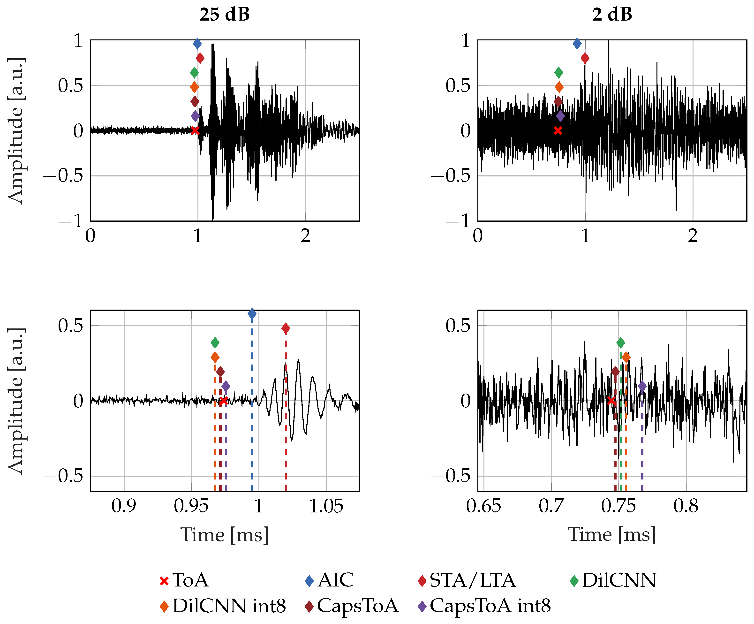
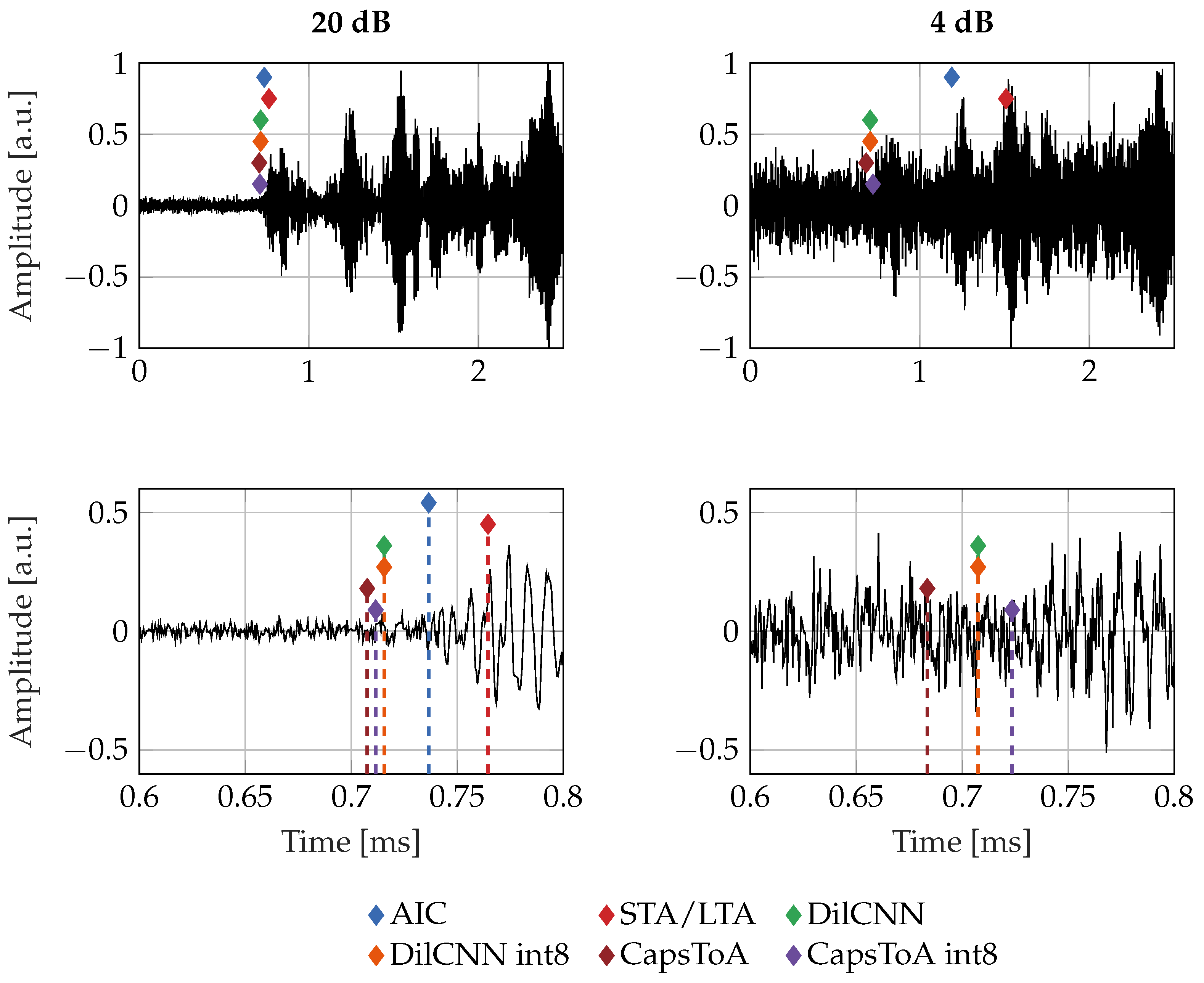
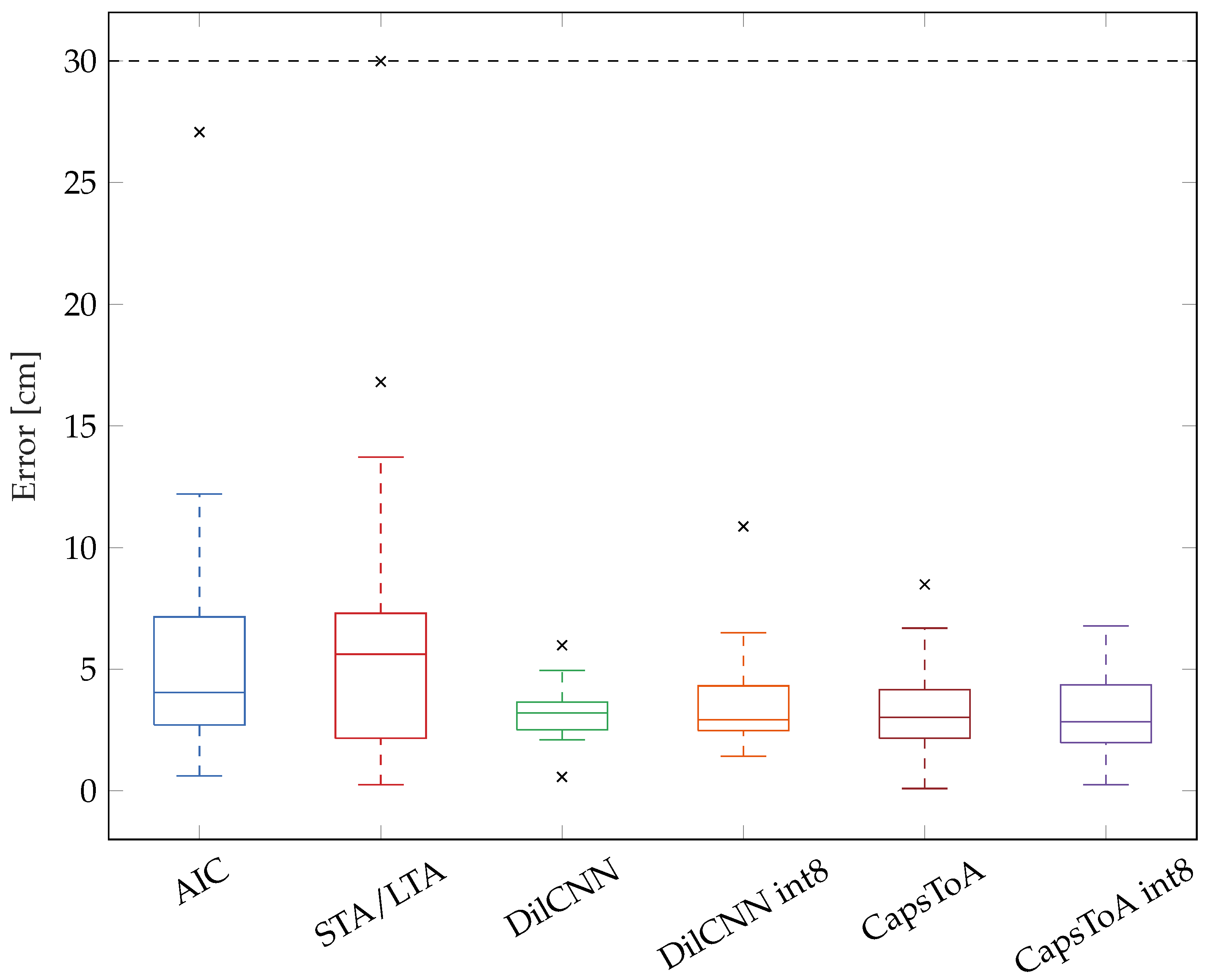
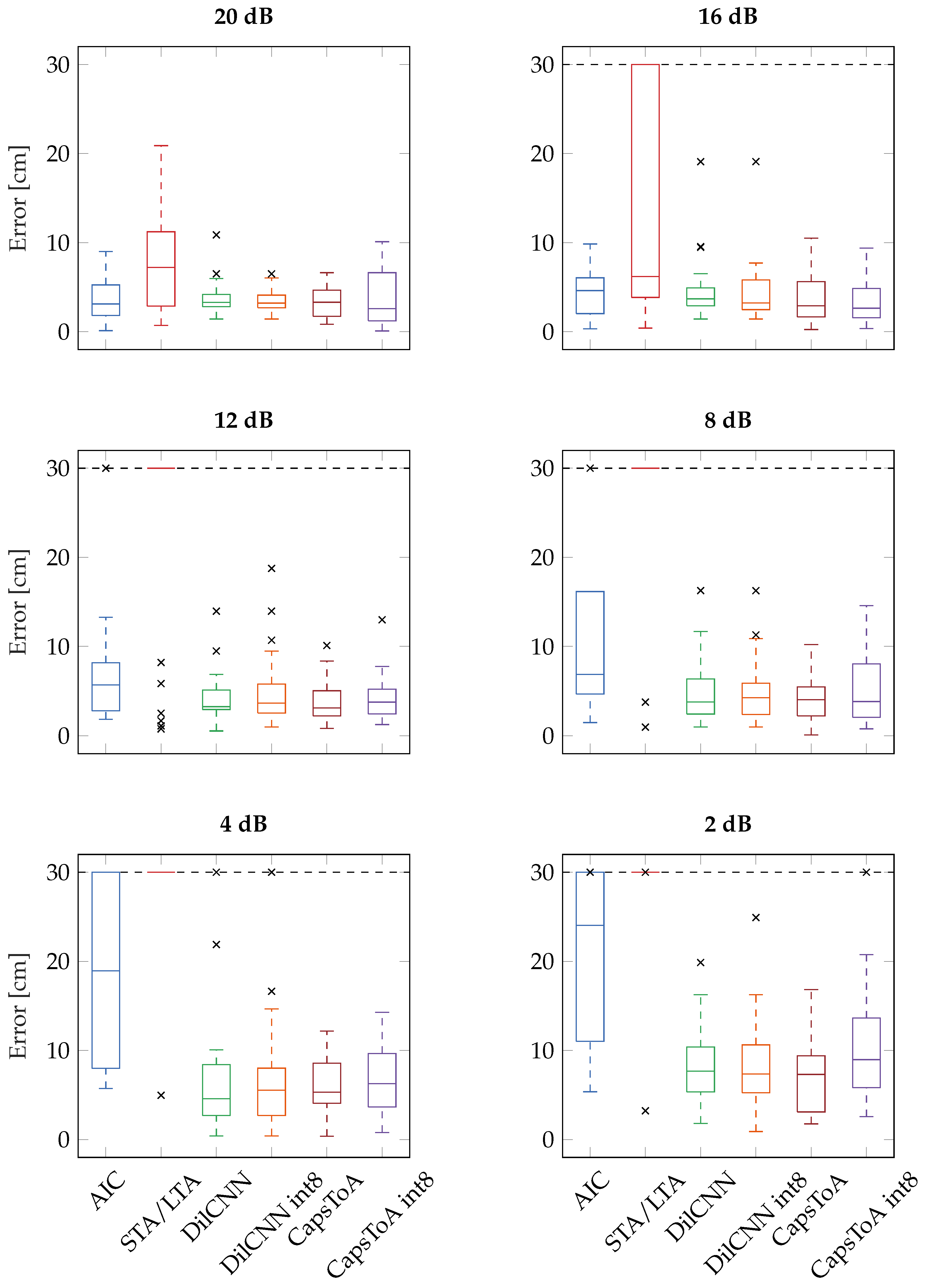
• We extensively validate the performances of the two novel models against various noise levels, proving their superiority in addressing two different tasks: (i) accuracy in the pure ToA estimation while working on synthetic data, (ii) precision in acoustic source localization for the experimental use case of a metallic aluminum plate; in particular, we will show that DilCNN and CapsNet can achieve a localization error which is up to 70% more accurate than STA/LTA and AIC even when the SNR is considerably below 4 dB;
• We implemented the devised NN models in a tiny machine learning environment and eventually deployed on a general-purpose and resource-constrained microprocessor, namely the STM32L4 microcontroller unit based on the ARM ^®Cortex-M4^®core: we demonstrate that these tiny variants score negligible loss of performances with respect to the full-precision alternatives.

2. Neural Network Architectures for ToA Extraction

In this section, the designed architectures are described in detail, along with the adopted methodologies and tools for their coding. To this end, all the NN models have been implemented and trained using Keras (https://keras.io/, accessed on 28 April 2023), a high level deep learning API built on top of the open source platform TensorFlow (https://www.tensorflow.org/, accessed on 28 April 2023) (TF).

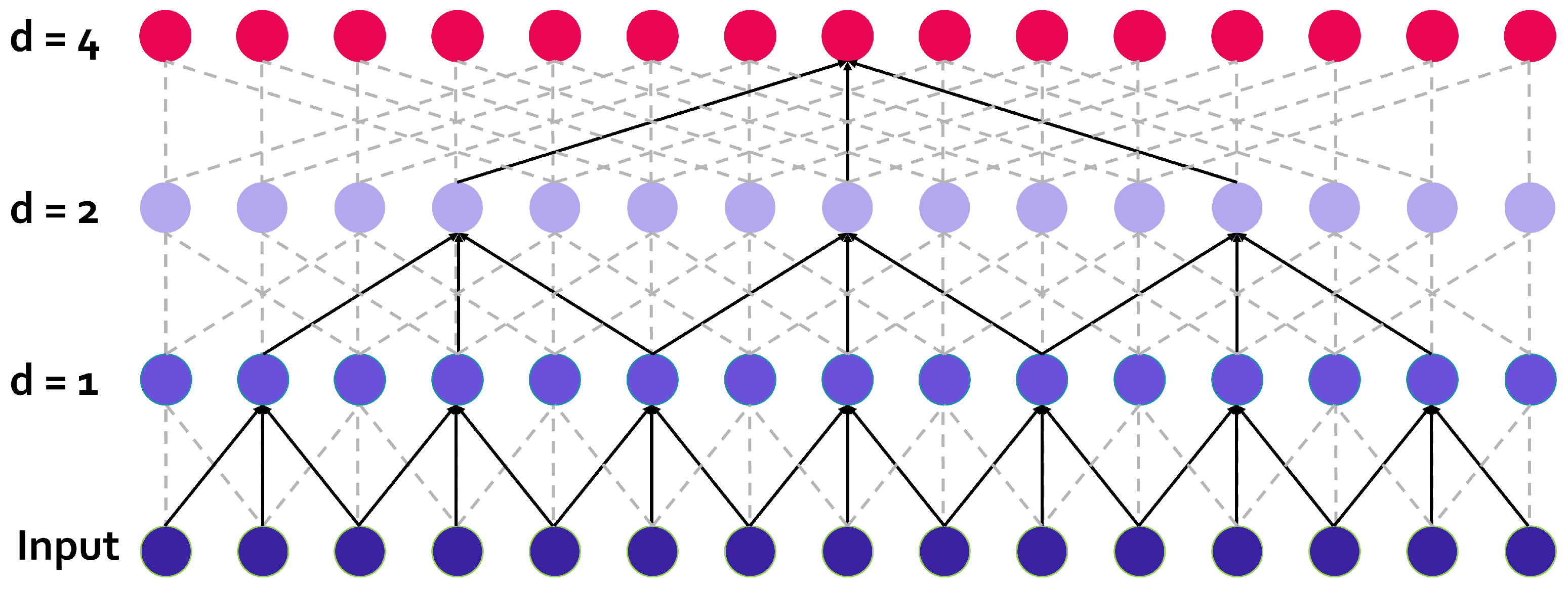
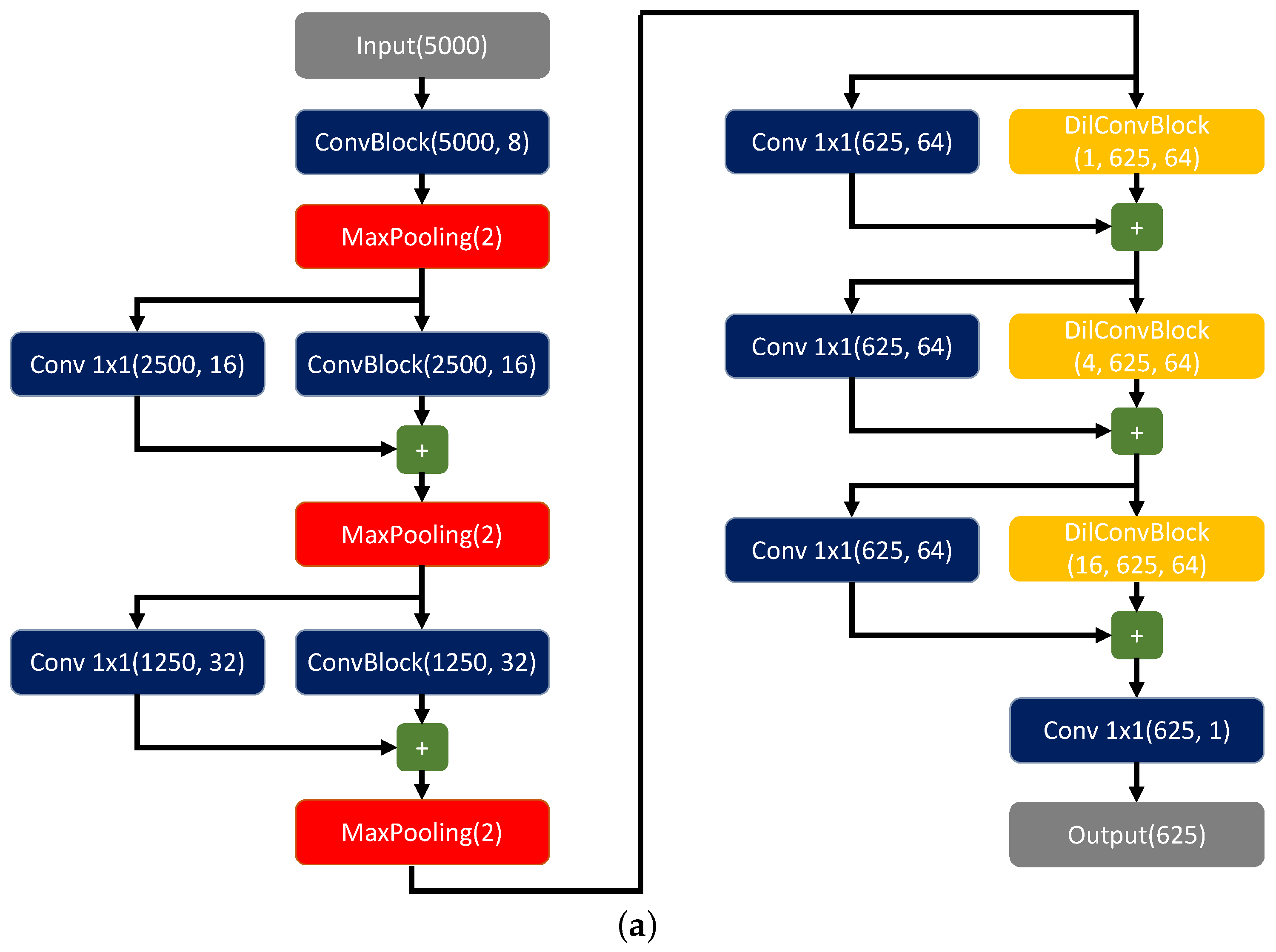
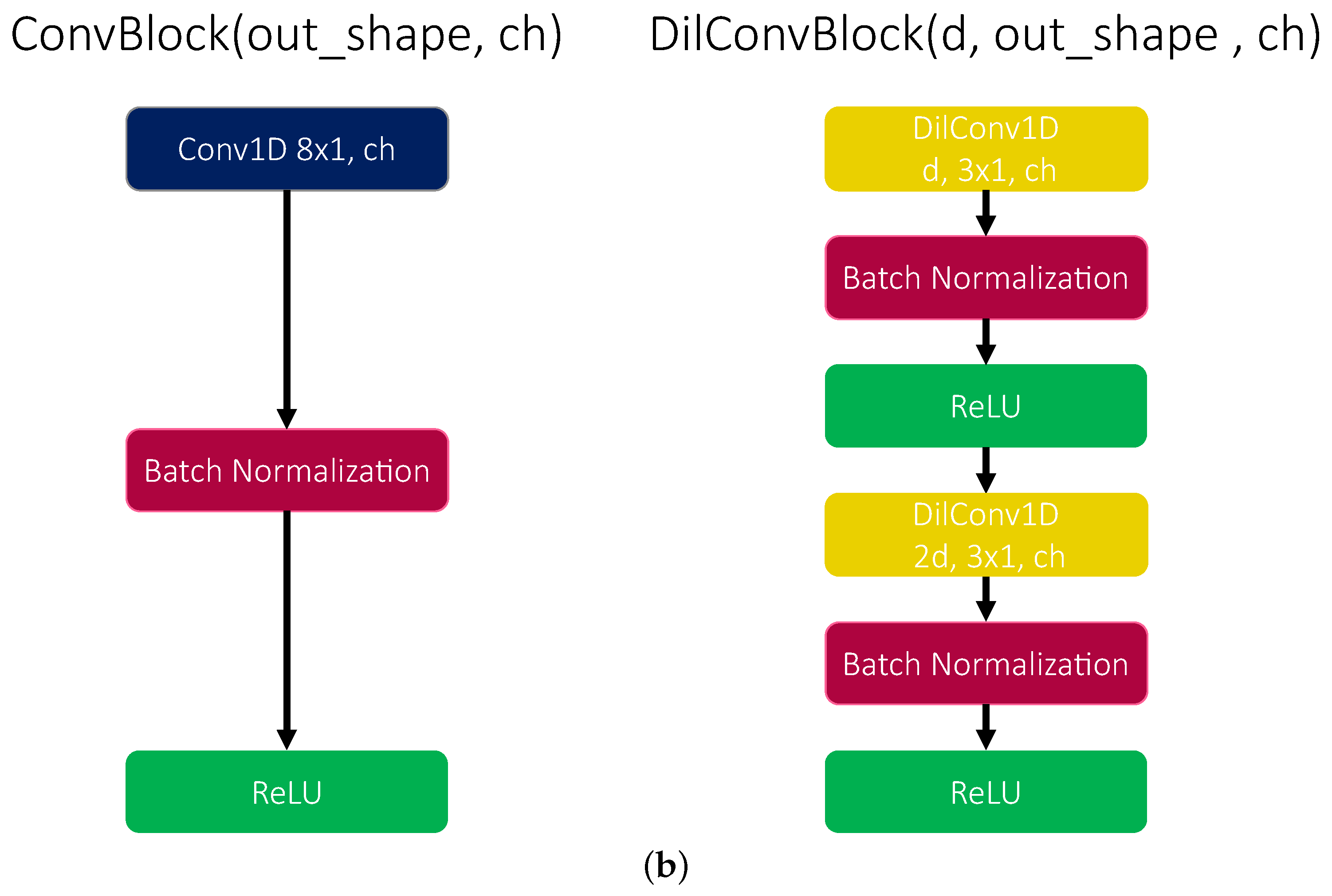
2.1. Dilated Convolutional Neural Networks

Convolutional neural networks (CNNs) are extremely popular DL models which have achieved impressive performance in a wide variety of applications, including images and time signal classification. Their functioning is inspired by the visual perception mechanism of animals [32]. CNNs extract relevant information from training data, preserving them in the form of linear filters (i.e., weights) and bias, which are applied to new inputs to obtain maps related to the spatial occurrences of informative features. In this way, weights are shared between different positions and the output of a convolutional layer is equivariant with respect to shift operations [33].

For problems involving the extraction of global information from data, such as image classification, a progressive undersampling of the input dimensions is performed by means of pooling layers of non-unitary stride: these aim at suppressing noisy or irrelevant features, while offering high level representations [33] and preserving computational resources. However, strides are associated with some undesirable drawbacks, such as the loss of temporal dependencies and the aliasing phenomenon, which might be particularly important for time series analysis. Hence, the solutions presented in [4,31], although being based on deep regression models with extremely low algorithmic burden, could not offer the optimal choice: the reason is that, for regression problems such as event picking tackled in this work, all the information related to the instant of occurrence of a specific feature might be lost due to the pooling layers and because of strides.

Consequently, to maximize the ToA prediction accuracy, it is mandatory to preserve temporal resolution whilst also considering a sufficiently long observation window, necessary to make each prediction aware of the full signal history. This means that the receptive field of a single output neuron associated to an input instant, defined as the patch of the input that affects its activation, should be wide enough. Considering a single path processed via a fully convolutional one-dimensional neural network, the receptive field $R{f}_L$ associated with a generic neuron at layer L is expressed by:

$$R{f}_L=\sum _{l=1}^L(k_l-1)\prod _{i=1}^{l-1}\mathrm{d}{t}_i+1$$

(1)

where $k_l$ is the kernel size of the l-layer while $\mathrm{d}{t}_i$ is the stride factor at layer i (${\prod }_{i=1}^{l-1}$ being the product operator). Another possibility to increase the network prediction capability is offered by the increment in the dimension of the kernel and/or in the number of hidden layers. However, for hardware-oriented applications in which spatial information must be preserved across the network and the neural models must be run on edge sensors with limited computational capabilities, this solution is not viable.

To overcome this issue, a more fruitful alternative is proposed in this work, which is based on the exploitation of dilated convolutional operators in place of the standard convolutional layers. There are several works in the literature which have proven the effectiveness of dilated kernels for the analysis of long time series with CNNs. Some examples are given by [34,35,36]. The key point behind dilated convolution (schematically depicted in Figure 1) is that certain weights are fixed to zero, hence introducing a sort of holes in the kernels. The spacing between non-zero coefficients is constant along each dimension and the associated dilation rate d is defined as the spacing plus one. It follows that, when $d=1$, conventional convolution is performed. Consequently, Equation (1) can be rewritten by replacing, in all layers, the kernel size k with a novel formulation $\tilde{k}$, reading as:

$$\tilde{k}=d(k-1)+1$$

(2)

By looking at Figure 1, it is notable that NN architectures based on dilated convolution can support exponential expansion of the receptive field without loss of resolution or coverage [37]. When the stride factor is fixed at 1 and the appropriate padding is applied, the dimension of the output is the same as that of the input.

The resulting model proposed in this study is presented in Figure 2a, while the structure of the constitutive building blocks is illustrated in Figure 2b; in the following, this network will be referred to as DilCNN. There are two constitutive elements in DilCNN. The first is a standard 1D convolutional block ConvBlock (left hand side of Figure 2a), defined by the output shape out_shape (fixed at $8\times 1$) and the number of channels ch, followed by batch normalization and ReLU activation function. The second is a 1D dilated convolutional block DilConvBlock of constant out_shape $3\times 1$, maximum dilation rate d and number of channels $ch$: for each dilation rate from $d_0=1$ to $d_f={log}_{2}d$, a sequence of 1D dilated convolutional layers plus batch normalization and ReLU activation is stacked.

The entire DilCNN is structured as follows. First, local features are extracted using convolutional blocks with unitary dilation rate. At the end of each block, a MaxPooling operator is introduced to suppress noisy information and reduce the computational complexity of the subsequent layers. Although such an operation implies a loss of temporal resolution, its effect become negligible when the number of MaxPooling layers is limited, in favor of a better compatibility with the tight constraints of low-end microprocessors. Then, local features are combined with a stack of non-causal dilated convolutions, to exploit both the past and the future trends of the signal which might be equally informative for our purposes. The dilation rate is increased exponentially after each layer, with an exponential basis equal to 2. Finally, the probability of the presence of an acoustic ToA in each timestamp is computed by means of a $1\times 1$ convolution (block named Conv $1\times 1$ in Figure 2a) activated by a sigmoid function.

The network is trained end-to-end using binary cross-entropy as a loss function, after converting each time label into a single hot vector of proper dimension. Nevertheless, this strategy might suffer from the same problems of unbalanced segmentation, i.e., the networks might tend to assign a score denoting the dominant class (the absence of an acoustic onset) to each timestamp: hence, a weight $W_p\ge 1$ is applied to the false negative term, leading to the loss function $L_{ce}$ in Equation (3):

$$L_{ce}=-\frac{1}{N}\sum _{i=1}^N{W}_p{y}_{i}log\left({\tilde{y}}_i\right)+(1-y_i)log(1-{\tilde{y}}_i)$$

(3)

with N being the number of samples, while $y_i$ and ${\tilde{y}}_i$ are the label and the prediction associated with instant i, respectively. Residual connections between different blocks are also added to avoid potential gradient losses, that may be a typical problem of deep NNs [39].

2.2. Capsule Neural Networks

CapsNets have been introduced in [18] to solve some of the intrinsic limitations of CNNs when solving image classification tasks. The latter can be summarized as follows: (i) CNNs have difficulties in generalizing to novel viewpoints [18]: the ability to deal with translation is built-in but, in the case of other affine transformations, we have to enlarge the training data with additional data samples that can provide knowledge about such new viewpoints; (ii) conventional CNN classification architectures rely on gradual undersampling of the input space, which can lead to the loss of significant information and spatial relationship between features [4,17], e.g., the classifier can be tricked and infer a false positive if an object in the scene has the same sub-components of the target but in different positions, thus belonging to a different class.

CapsNets overcome these issues by: (i) using transformation matrices that learn how to encode the intrinsic spatial relationship between a part and a whole, ensuring better generalization capabilities, (ii) substituting scalar activations by vectors which are equivariant with respect to the transformations to be applied to the input [18,40]. Another non-negligible benefit of CapsNets is their ability to learn from comparatively smaller datasets, preserving salient data information such as position and location [17].

A CapsNet architecture is typically stacked on top of a convolutional network, which is in charge of local feature extraction and consists of the following two layers:

• Primary Capsule Layer: the first component of this layer is a convolutional operator with a number of channels $M_{PC}\times D_{PC}$, where $M_{PC}$ indicates the number of primary capsules per spatial—or temporal—position. Thus, the output of this operator is reshaped, starting from the channel dimension, into a set of $N_{PC}=K\times M_{PC}$ vectors $s_i$ with $D_{PC}$ coordinates, which are the so called primary capsules $u_i$, with K being the number of temporal positions. These primary capsules are activated by means of a non-linear squash function and finally mapped into a probability value, according with [18]:

  $$u_i=\frac{\left|\right|s_i{\left|\right|}^2}{1+\left|\right|s_i{\left|\right|}^2}\frac{s_i}{\left|\right|s_i{\left|\right|}^2}$$

  (4)
• Capsule Layer: each primary capsule ${\widehat{u}}_i$ with $i\in \{1\dots N_{PC}\}$ generates a prediction $u_{i|j}$ for every j-th class—with $j\in \{1\dots N_{class}\}$—by means of a weight opinion matrix $W_{ij}$:

  $${\widehat{u}}_{i|j}=W_{ij}{u}_i$$

  (5)
  Such opinion matrices are learned during training and encode the relationship between local low-level features and the high-level entities associated with classes; hence, they are invariant to transformations applied to the input. In this way, capsules provide a simple way to detect global features by recognizing the individual contributions of the parts [40]. A global prediction $p_j$ for each class is, indeed, computed as a linear combination of the vectors obtained via Equation (5), yielding to:

  $$p_j=\sum _{i=1}^{N_{PC}}{c}_{ij}{\widehat{u}}_{i|j}$$

  (6)
  Individual $p_j$ are then activated by the squash function in Equation (4). Coefficients $c_{ij}$ are determined following the dynamic routing protocol [18]. This consists of an iterative process, summarized in Algorithm 1, which combines together the output $v_j$ of single capsules with the appropriate parent belonging to the layer above. The pairing procedure works as follows: if ${\widehat{u}}_{i|j}$ has a large scalar product with the global output of a possible parent class, there is a top-down feedback which increases the coupling coefficient for that parent while decreasing it for the other ones. It follows that the higher the norm of an output vector, i.e., the higher the level of agreement between low-level capsules which are associated with its parts, the higher the likelihood that the corresponding feature class describes the input data.

  Algorithm 1 Dynamic Routing

  for all capsule i in layer l and capsule j (i.e., class) in layer $(l+1)$: $bij\leftarrow 0$ for r iterations do    for all capsule i in layer l: $c_{ij}\leftarrow \mathbf{softmax}\left(b_{ij}\right)=\frac{exp\left(b_{ij}\right)}{{\sum }_{k}exp\left(b_{ik}\right)}$    for all capsule j in layer $(l+1)$: $p_j\leftarrow {\sum }_i{c}_{ij}{\widehat{u}}_{i|j}$    for all capsule j in layer $(l+1)$: $v_j\leftarrow \mathbf{squash}\left(p_j\right)$    for all capsule i in layer l and capsule j in layer $(l+1)$: $bij\leftarrow bij+{\widehat{u}}_{i|j}·v_j$ end for return $v_j$ for all capsule j in layer $(l+1)$

The margin loss was used as cost function during training, since it can sum together the components related to individual classes:

$$L_{margin}=\sum _{a=1}^{N_{class}}{T}_{a}max(0,m^{+}-\left|\right|v_a{\left|\right|)}^2+\lambda (1-T_a)max(0,||v_a\left|\right|-m^{-}{)}^2$$

(7)

where $T_a=1$ if class a (a being 1 or 0) is present, while $m^{+}=0.9$, $m^{-}=0.1$ and $\lambda =0.5$ are tunable hyperparameters.

In this work, $r=3$ has been imposed after an appropriate tuning of this parameter. CapsNets based on dynamic routing can solve classification problems where it is reasonable to assume that, at most, only one instance per class is present in the input scene [18]. Accordingly, in our scenario, only one wave arrival is supposed to be present in each processed time series, which are thus split into overlapped windows of length $N_w=400$: label 1, corresponding to class $AE$, is assigned only when a data point has no samples preceding ToA, i.e., it is fully contained into the time slot corresponding to the target acoustic event and not into its pre-onset temporal sequence; otherwise, class $Noise$ (label 0) is attributed, indicating noisy windows. The task solved by the designed CapsNet is, thus, to perform a binary classification distinguishing between these two classes, i.e., AE event or noise. Hence, dedicated post-processing logic has to be applied to extract the sought ToA.

Similar to the solutions adopted in [4,16,17,41], predictions are formulated by computing the probability curve related to the $AE$ class, i.e., sliding a window with a constant stride and calculating the norm of the output vector corresponding to such a class for each shift. The stride factor has been selected equal to the pooling factor of the feature extraction layers in the DilCNN model (i.e., 8), in order to obtain a fair comparison between the two networks using the same temporal resolution. To this end, a dilated CNN, similar to the one presented in Section 2.1 but without the first three $d=1$ convolutional layers followed by MaxPooling and different number of channels (i.e., 16, 32 and 64), has been considered: in this way, it is possible to detect the window containing the onset of the signal without relying on less generalizable and prone to noise methods such as simple thresholding schemes. The overall CapsNet model, henceforth denoted as CapsToA, is illustrated in Figure 3: in particular, Figure 3a shows the capsule neural network adopted for the classification of windows: in convolutional blocks, kernel dimensions, output shape and number of channels are reported; for the 1D convolution used in the primary capsule layer, 32 $4\times 1$ kernels are used, reshaping the output tensor into 200 capsules with 8 dimensions. All stride factors are set at a value of 2. The post-processing dilated CNN is instead reported in Figure 3b. The two models are trained separately and the input of the latter is constituted by the time sequence obtained by concatenating $AE$ class predictions related to adjacent windows. Since no padding is applied and input signals consist of 5000 samples, such a curve is composed of a $(5000-N_w)/stride+1=(5000-400)/8+1=576$ timestamp.

Given these computational complexity, a naive CNN with no attention mechanism has been imposed to implement the convolutional layers forming the input block of the CapsNet architecture (dark blue rectangles in Figure 3a). Similarly, a dynamic routing algorithm is exploited in its earliest formulation [18] as performed in [4,16,17,41]. Such a minimal approach is justified by the fact the our CapsNet should be executed 576 times for each time series in order to produce the output probability curve. By doing so, we are not aiming at proposing a novel DL architecture, a challenge which is out of the scope of the work, but rather at establishing an effective framework based on CapsNet by introducing an ad hoc post-processing strategy for the retrieval of the ToA.

2.3. Quantization Schemes

Models have to be converted into MCU-compliant and low-depth format (i.e., 8-bit) to be portable on edge devices. This procedure, referred to as quantization, is crucial to provide a significant reduction in both the memory footprint and computational complexity, especially considering the critical resource constraints which characterize tiny embedded devices with low-power consumption. Another fundamental reason supporting the necessity of quantization is that a great number of hardware platforms widely used in DSP applications are equipped with instruction sets (ISAs) which are optimized for sub-word operands [42]: this means that a single instruction can be applied simultaneously to multiple operands with a bit resolution smaller than the parallelism of the data bus. However, the conversion of weights and activations into int8 type could lead to performance degradation due to the lower representation capability provided by the NN models. Techniques have been developed to minimize the effect of this unavoidable operation.

In general terms, a quantization scheme can be defined as the mapping between the bit-representation of values (denoted q in the following) and their interpretation as real mathematical numbers (r) [43]. Quantization procedures are typically implemented using integer-only arithmetic during inference and floating-point arithmetic at training time. We refer to post-training quantization (PTQ) when the model is converted into a lower precision representation after a training process consisting of a stochastic gradient descent implemented in floating point via a backpropagation algorithm. An alternative to this approach is the so called quantization-aware training (QAT), in which trainable parameters, i.e., weights and biases, are updated in floating point arithmetic as usual, while the forward propagation necessary to the computation of the loss for each batch relies on fake-quantization layers. The latter are used to emulate non-linear noise introduced by the desired compression of weights and activations by means of a rounding mechanism [43,44]. QAT has the advantage of totally preserving the accuracy of the model after conversion, but typically leads to longer training time [44,45] and could imply a worse overall performance with respect to PTQ. For such reasons, only PTQ will be adopted in this work: it has been implemented in a static fashion, meaning that activation ranges are calculated during model conversion from a reduced batch of sample data, allowing quantization parameters to be calibrated without introducing any overhead at runtime.

To accomplish this, public open source libraries have been used. In more detail, DilCNN models were quantized by means of TensorFlow Lite (https://www.tensorflow.org/lite, accessed on 27 April 2023) (TFLite), a framework for deploying TF models on mobile and other edge devices, also providing a specific library for execution on MCUs (the TensorFlow Lite for Microcontroller framework (https://github.com/tensorflow/tflite-micro, accessed on 27 April 2023) or TFLite-Micro) including 8-bit kernel implementations of the majority of the Keras layers and TF built-in operators. TFLite-based quantization uses integer-only arithmetic without relying on a fixed-point format for the purpose of value conversion: it applies an affine mapping of integers q to real numbers r [43] according with:

$$r=S(q-Z)$$

(8)

where S is a floating point number denoted as a scale factor while Z is the integer zero-point. This quantization scheme uses the same quantization parameters for all values within each activation or weight array. Hence, separate arrays use different quantization parameters. Weights of dilated convolutional layers have been mapped as pair of values $(S,Z)$ (corresponding to per-axis or per-channel conversion), since this can reduce the impact of quantization [46].

Such parameters (S and Z) depend both on the number of bits adopted in the quantized layer and on the numerical range covered by a tensor. For this reason, while the ones associated with weights can be derived directly from the trained model, a representative set of input data is required in order to calibrate the ones related to activations for the case of static PTQ. For further details, the reader is referred to [43] and to the TFLite documentation for 8-bit quantization (https://www.tensorflow.org/lite/performance/quantization_spec, accessed on 27 April 2023).

Conversely, for the 8-bit implementation of the CapsNet architecture, we rely on the framework proposed in [46] (https://gitlab.com/ESRGv3/q7-capsnets, accessed on Thursday, 27 April 2023), which provides a ready-to-use library for the edge execution of capsule Layers on Arm^®Cortex^®-M and RISC-V MCUs, along with a quantization tool in the Python environment compatible with models developed in Keras. This library developed for Cortex-M is an extension of CMSIS-NN [47] and implements 8-bit optimized kernels for matrix multiplication which uses the single instruction–multiple data (SIMD) features of Armv7E-M and Armv8-M architectures for multiply-and-accumulate (MACC) operations. Since the related ISAs do not feature 4 × 8-bit MACC operands, they rely on 2 × 16-bit MACC performed after a sign extension.

Unlike the TFLite framework, a fixed-point notation with power-of-two scaling is used in this case for the quantization of trainable parameters and activations, i.e., each tensor is associated with a $Q_{m.n}$ format where m is the number of integer bits while the remaining n are considered for the fractional part. It is important to note that $m+n=7$ since the last bit is used for the sign. The framework proposed in [46] enhances the precision in layers with very small weights by virtually increasing the number of fractional bits: every weight still fits in 8 bits, but the quantization format can, virtually, surpass this barrier. Once the right fixed-point formats are defined, weights and biases are appropriately scaled and clipped into the range [−128, 127]. Then, the amount of bit-wise shifts which should be applied after each fixed-point matrix operations is calculated. Nevertheless, the output probability related to the AE class is retained in a 32-bit format in order to avoid the saturation of the curve, which would complicate the extraction of the ToA, then rescaled into an 8-bit representation via Equation (8) before passing through the subsequent DilCNN model. The final DilCNN-based ToA logic has been quantized analogously to the previously described DilCNN by means of the TFLite framework, since the two models of CapsToA are trained separately and then stacked together.

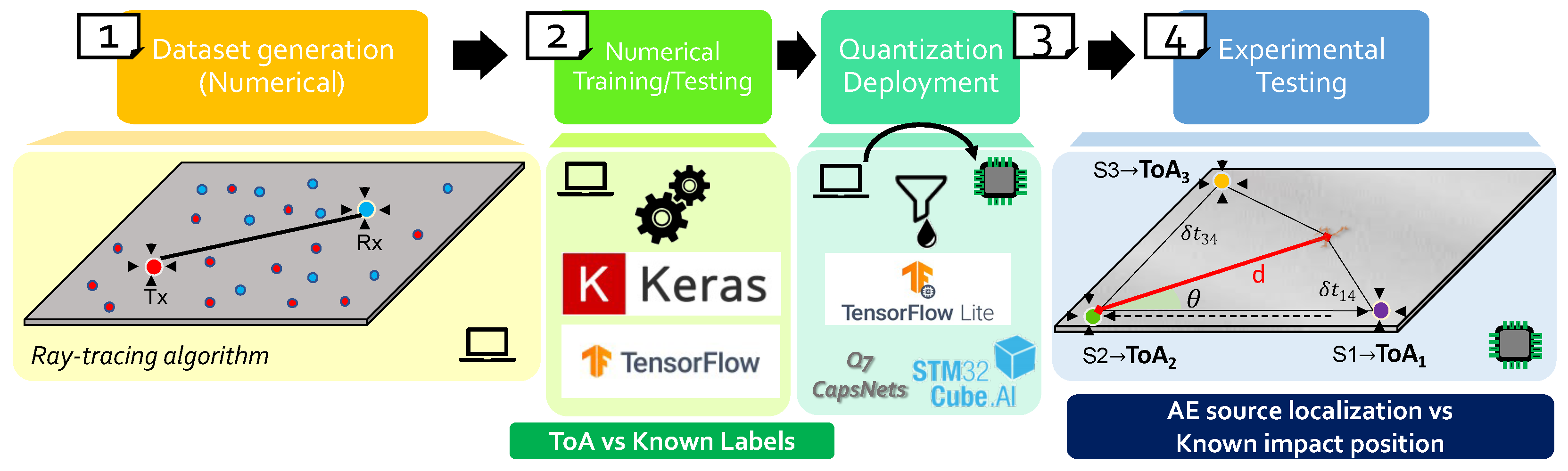
3. Model Deployment Process, Training and Testing

The entire validation flow, from dataset generation to model testing, for the task of AE localization from real-field data is schematically represented in Figure 4.

3.1. Materials

The STM32L496ZGT-P Nucleo board [48] equipped with an ARM ^®-Cortex^®M4 core and maximum clock frequency of 80 MHz has been employed for prototyping purposes. It features 1 MB of FLASH memory and 320 KB of SRAM, which are compatible with the typical characteristics of edge nodes to be deployed for long-lasting SHM monitoring. The X–CUBE–AI expansion package (https://www.st.com/en/development-tools/stm32cubemx.html, accessed on 2 May 2023) has been used as a development environment for the embodiment of the sought models.

3.2. Dataset Generation

The dataset for the training phase has been built via numerical simulations (step 1 in Figure 4). This procedure based on synthetic AE signals has been preferred over a purely experimental approach for two main reasons: the first is that it allows the data collection phase to speed up, since a relatively short amount of time is necessary to generate a representative pool of data; secondly, and more importantly, it permits the fast creation of ground truth labels for supervised learning (as is the case of the adopted solutions), a condition which is not applicable in passive AE monitoring scenarios where the true AE triggering time is always unknown to the sensing system.

When an AE event occurs in a waveguide as a consequence of crack, corrosion or delamination, the corresponding release of energy can travel along the structure in the form of ultrasonic guided waves (GWs). The propagation characteristics of GWs can be numerically modeled when the geometrical and mechanical parameters of the monitored structure are known. To this end, an ad hoc ray-tracing algorithm has been exploited in this work, which simulates the peculiar propagation behavior of GWs between different combinations of points on a thick aluminum plate while also taking into consideration the effects of multiple reflections due to the mechanical boundaries.

Moreover, it is worth mentioning that the generation of a custom dataset was imposed by the absence, to the best of the authors’ knowledge, of public benchmarks which specifically address the same problem. Indeed, only a few AE data collections have already been released in the literature, such as the ORION-AE (https://dataverse.harvard.edu/dataset.xhtml?persistentId=doi:10.7910/DVN/FBRDU0, accessed on Tuesday, 2 May 2023) and the Hsu-Nielsen on concrete blocks (https://www.sciencedirect.com/science/article/pii/S2352340919301647#sec1, accessed on Tuesday, 2 May 2023) dataset. The former represents a collection of time series reproducing the bolt loosening effect typical of assembled appliances. However, despite the huge amount of data acquired during this campaign, there are two main factors hindering its applicability in our SHM framework: (1) the acquired measurements, namely vibrations, which reflect the dynamic response of the structure, whereas we considered AE signals emitted as a consequence of long-aging static stress; (2) the absence of labels, which are mandatory for the implementation of the supervised DL models we have investigated. The latter, instead, contains bulk acoustic waves collected by conducting pencil lead break tests on a concrete block. As such, the nature of the involved AE signals differs largely from the one considered in our work. The main difference is that, while bulk waves have only two propagation modes (longitudinal and shear) and can be used to inspect small areas in the neighborhood of the AE transducers, Lamb waves can travel comparatively longer distances, showing a multi-modal pattern (i.e., multiple symmetric and asymmetric modes are excited and propagate at the same time) and suffering from interaction with the boundaries of the structure.

The entire number of combinations between the selected points for AE actuation and reception has been chosen randomly, while also changing the SNR into the set $\{1,2,4,6,8,10,12,15,18,20,25,\infty \}$ for a total amount of 60,000 time series: 80% of this data was used for training and validation and the remaining 20% was allocated to testing.

3.3. Validation Process

The performance of the different models has firstly been assessed on the synthetic testing dataset (12,000 time series) introduced in Section 3.2 (step 2 in Figure 4). Mean absolute error (MAE) and root mean square error (RMSE) are used in this first validation step as performance metrics. Then, once quantized and deployed on the target STM32L4 MCU (step 3 in Figure 4), the ToA prediction algorithms have also been tested for localization purposes in an experimental setting (step 4 in Figure 4) involving a thin aluminum plate ($1000\times 1000\times 3\mathrm{mm}$) instrumented with three custom sensor nodes (installed on three corners of the structure) developed within the Intelligent Sensor Systems lab of the University of Bologna and located at as many corners of the structure (see Figure 5). Thanks to the compact design including all the circuitry and electronics necessary to collect, pre-process and characterize signals, each device works as a miniaturized oscilloscope capable of acquiring, at the same time, signals on three different input channels with a capacity of 4 MS/s. All the details about the sensor node characteristics can be found in [49,50]. This plate has been selected since it presents identical mechanical and geometrical properties to the one adopted for numerical simulations; thus, it allows the exploitation of the same NN models trained on the simulated time series.

Nine different positions have been considered for excitation: each test has been repeated three times, for a total amount of 27 tests. The adopted sensor installation plan is compatible with the triangulation method in [51], whose complete mathematical formulation can be found in [4]: the algorithm is advantageous in that, thanks to simple geometrical considerations, it allows the retrieval of a source position simply by knowing the difference in ToA of three sensing units placed at known positions. Such a testing procedure was necessary since, as anticipated, it is not possible to make an educated guess about the true label in the case of a real-field scenario due to the passive nature of AE monitoring. In these terms, localization offers an indirect means for quantifying the performances in ToA estimation by computing the spatial error between the true impact position and the estimated one.

Furthermore, since the primary advantage of AI approaches is that they can efficiently learn patterns even in very noisy data, the impact of progressively increasing noise levels on the predicted ToA was specifically evaluated. To this end, gathered data were corrupted with an additive white Gaussian noise (AWGN) such that the corresponding SNR moves from 20 dB to 2 dB at integer steps of 4 dB. Despite the fact that the nature of the background noise of real AE signals can differ [5], additive white stationary noise (such as that generated by electronic components) can be assumed to be the main source of SNR degradation and, consequently, was used to simulate noisy AE scenarios in this study.

4. Results

4.1. Preliminary Validation on Synthetic Signals

Results on synthetic waveforms are summarized in

Table 1. MAE and RMSE in ToA identification (expressed in μs) for different SNR intervals. Performances of the two NNs are reported both for floating point Keras models and for the int8-quantized versions, with the exception of the CNN architecture which is included just for comparison purposes. Best results for each SNR and metric are highlighted in bold font.

Method	SNR [dB]	MAE [μs]	RMSE [μs]
AIC	≥20	29.47	40.10
	12–20	68.96	89.02
	6–12	115.47	133.79
	<6	132.74	151.74
STA/LTA	≥20	59.56	106.23
	12–20	150.38	213.31
	6–12	229.00	321.83
	<6	301.88	401.31
CNN	≥20	138.68	373.21
	12–20	138.45	372.88
	6–12	138.43	372.86
	<6	138.82	373.40
DilCNN	≥20	8.29	29.98
	12–20	8.25	29.89
	6–12	8.23	29.81
	<6	8.24	29.78
DilCNN int8	≥20	8.27	29.93
	12–20	8.24	29.85
	6–12	8.22	29.77
	<6	8.26	29.79
CapsToA	≥20	7.63	11.4
	12–20	10.15	14.41
	6–12	14.54	28.51
	<6	25.56	55.72
CapsToA int8	≥20	16.39	23.68
	12–20	19.81	50.29
	6–12	22.46	32.05
	<6	43.79	71.08

, for different intervals of SNR. The performances attained by AIC and the STA/LTA-based thresholding algorithm are also reported. In the latter case, the ratio between the two moving averages is computed on the absolute value of Hilbert-transformed signals: ToA was retrieved as that time index for which the threshold is exceeded first. Such a threshold was fixed at 10 while the two window lengths (5 and 250, respectively) were empirically tuned on a subset of training data. Importantly, we have also included the accuracy in ToA estimation attained by a standard CNN architecture having the same structure (i.e., identical number of parameters, computational complexity and hyperparameters) of the DilCNN model, but replacing dilated kernels with conventional convolutions. Some examples of simulated waveforms with the relative predictions are showed in Figure 6.

As can be observed from Table 1, all the new DL models investigated in this work widely outperform other statistical or threshold-based methods, especially in the presence of high noise levels. In more detail, DilCNN is quite insensitive to noise, obtaining very similar MAE and RMSE for all the considered SNRs. The superiority of dilated convolutions over conventional ones has also been proven, as witnessed by the fact that CNN scores were more than 16 times worse in all the configurations, eventually being less effective than the AIC algorithm. This result is justified by the fact that, despite sharing the same architecture, the receptive field of the output neurons in CNN (computed via Equation (1) assuming the architecture size in Figure 2) is equal to 153 samples (i.e., $76.5$ μs), nearly seven times smaller than the one characterizing DilCNN, which amounts to 1065 samples (corresponding to $532.5$ μs). Thereby, in the following analyses, only results for dilated convolutional architectures will be presented. Moreover, it is paramount to emphasize that its quantized version (DilCNN int8) scores the same accuracy levels, with a negligible loss of performance. CapsToA behaves comparatively better than AIC and STA/LTA, even if proving to be more sensitive to noise disturbances. A slight degradation is noticeable for its MCU implementation (CapsToA int8), but it still reaches significantly better metrics (both for MAE and RMSE) than the alternative DL-free solutions, as demonstrated by an average gain of 30× for the whole set of noise ranges.

Additionally, the computational complexity, intended as the number of MACC operations, was also estimated, together with the overall execution time (expressed both in clock cycles $T_{ck}$ and $\mathrm{m}\mathrm{s}$) and the RAM and flash footprint of the generated models when run on the STM32L4 MCU. All these values are summarized in

Table 2. System performance of the analyzed models with 8-bit numerical precision while running on the target STM32L4 MCU at 80 MHz clock frequency.

Model		SRAM	Flash	MACC	Tck	Tck/MACC	Exec Time
		[KB]	[KB]				[ms]
DilCNN int8		171.50	120.27	59,120,625	332,758,980	5.628	4159.359
CapsToA int8	CapsNet	16.18	54.14	280,032	2,076,305	7.415	25.954
	DilCNN	136.00	49.50	15,750,720	147,491,915	9.364	1843.551
	Overall	152.18	103.64	177,049,152	1,343,443,595	7.588	16,793.044

and are provided only for the int8 quantized models, since they are the only DL architectures running on the target embedded platforms; hence, these defining parameters are of crucial interest.

By looking at Table 2, it is possible to observe how differences in kernel implementations affects the computational efficiency of our networks. In fact, TFLite micro kernels used for the implementation of DilCNN models performs much faster in case of conventional convolution when compared to dilated convolution, as demonstrated by the difference in the T_ck/MACC ratio between the first model and the DilCNN-based post-processing logic adopted in the CapsToA architectures: the reason is that the former distributes its complexity mainly on $d=1$ convolution operations, unlike the latter.

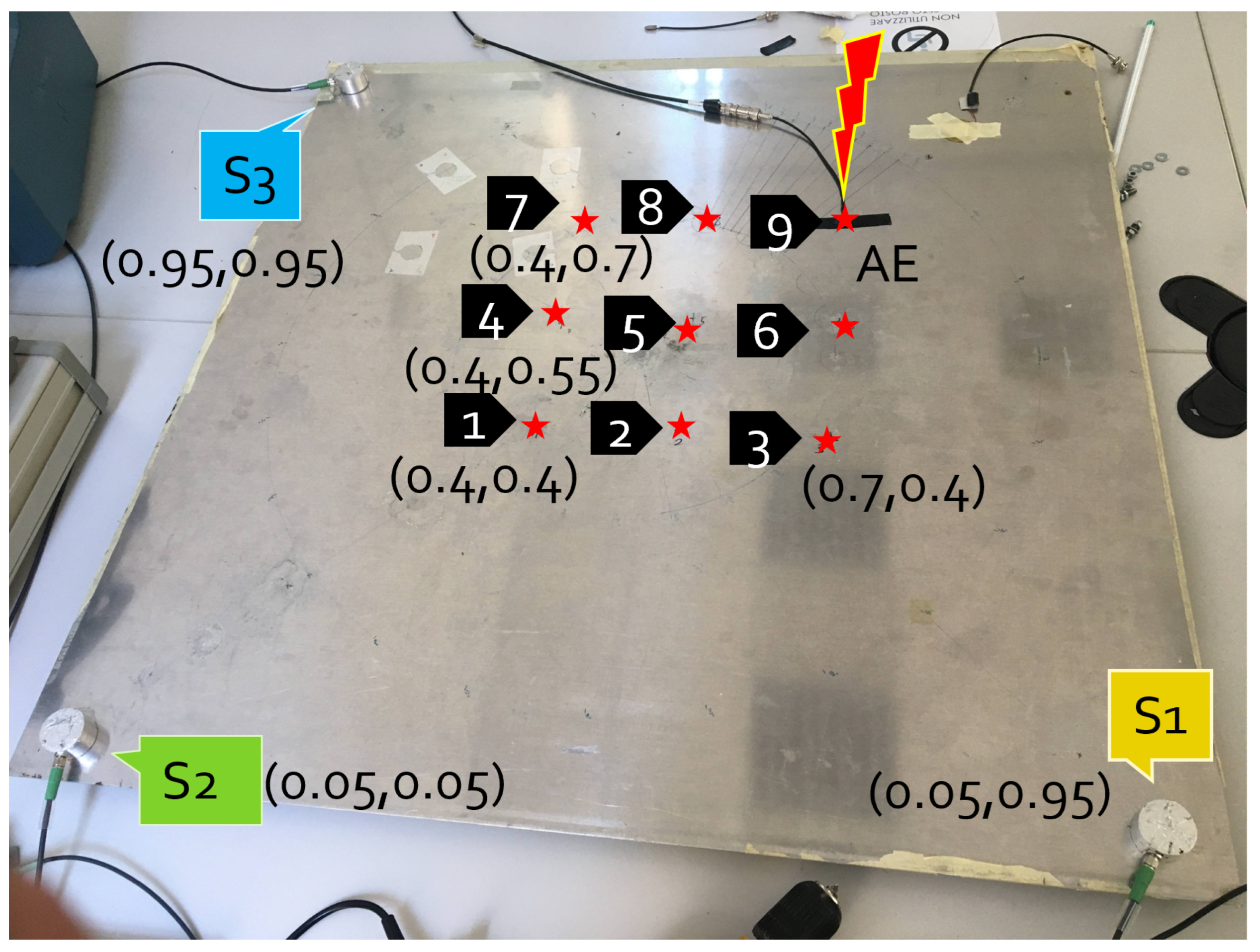
4.2. Real-Field Validation for AE Localization

In this section, the results in terms of localization accuracy when dealing with real-field data are presented, by sweeping the SNR. Figure 7 reports some examples of collected signals, along with the predictions obtained by using the different identification, which are better magnified in the second row in which a zoomed interval is depicted.

Results for source localization are statistically analyzed in Figure 8 in terms of boxplots for the noise-free configuration, while Figure 9 summarizes the outcomes when testing on signals corrupted by increasing levels of artificial AWGN added via software elaboration. Boxes are limited between the 25th and 75th percentiles of the sample data, while the horizontal line stands for the statistical median. Data points marked with a black cross are outliers, which are identified as those values greater than $q_3+1.5(q_3-q_1)$ or less than $q_1-1.5(q_3-q_1)$, where $q_1$ and $q_3$ are, respectively, the 25th and 75th percentiles. The dashed vertical extrema of each box represent the whiskers.

Moreover, it is important to mention that large errors in ToA identification may lead to non-physical configuration in which a possible source location does not exist analytically or it is located out of the geometrical boundaries of the plate: when this applies, the corresponding tests has been denoted as failed. The different failure rates, expressed as the ratio between the total number of failed tests over the total amount of performed experiments, are summarized in

Table 3. Median values and percentages of failed tests obtained with the different methods by varying the signal-to-noise ratio. Best results for each SNR are highlighted in bold font.

Model	Metric	∞	20 dB	16 dB	12 dB	8 dB	4 dB	2 dB
AIC	Median [cm]	4.05	3.12	4.62	5.68	6.85	18.93	24.03
	Failure Rate	0%	0%	0%	7.7%	23.1%	34.6%	23.1%
STA/LTA	Median [cm]	5.62	7.23	6.21	Failed	Failed	Failed	Failed
	Failure Rate	3.8%	0%	34.6%	76.9%	92.3%	96.2%	88.5%
DilCNN	Median [cm]	3.21	3.3	3.69	3.24	3.76	4.58	7.67
	Failure Rate	0%	0%	0%	0%	0%	0%	0%
DilCNN int8	Median [cm]	2.92	3.22	3.23	3.64	4.24	5.54	7.36
	Failure Rate	0%	0%	0%	0%	0%	0%	0%
CapsToA	Median [cm]	3.02	3.32	2.92	3.09	4.01	5.32	7.31
	Failure Rate	0%	0%	0%	0%	0%	0%	0%
CapsToA int8	Median [cm]	2.84	2.6	2.64	3.75	3.81	6.27	8.97
	Failure Rate	0%	0%	0%	0%	0%	0%	7.7%

, for each algorithm and SNRs; median values in localization accuracy are also displayed.

The above results confirm again the superiority of DL models in dealing with critically noisy scenarios with respect to traditional methods. Indeed, these charts validate that, for all the considered noise configurations, both the failure rate and source position estimation are significantly improved when AI model solutions are considered, AIC and STA/LTA being affected by (i) a remarkable statistical dispersion (larger boxplots) and (ii) much lower success rate. For example, when the SNR is equal to or below 4 dB, the median error values reached by the lower performing quantized neural model, i.e., CapsToA int8, decrease more than 66% and 62% at 4 dB and 2 dB, respectively, when compared to AIC-related scores (which is the most accurate amidst the two conventional algorithms). The proof is the fact that, opposite to its quantization-free version, CapsToA int8 undergoes a penalty on median value of about 17.9% at 4 dB and 22.7% at 2 dB after quantization.

DilCNN presents a moderate performance degradation as the noise level increases, as opposed to behavior observed in the case of synthetic AE signals. This might be due to the slight difference between the simulated and the actually measured data, as evident by comparing the waveforms in Figure 6 and Figure 7. However, between the two DL networks, DilCNN is the one which shows the best accuracy at low SNRs after conversion to 8-bit precision, with a maximum degradation in the median value below 21% and 48% for the worst case situation of SNR = 4 dB. All these experimental observations further corroborate the quality of the previously quantified results obtained in the case of analytical frameworks, disclosing novel opportunities for sensor-near AE signal characterization and defect localization.

5. Discussion

In

Table 4. Comparison of results obtained in this work with respect to state-of-the-art approaches in the field of AE source localization. Pros (✓) and cons (✗) of each method are discussed, along with their quantitative performances in terms of magnitude of localization error (assuming that no additional synthetic noise is inserted) and integration on extremely low-level computing devices.

Ref.	Model	MCU Deployment	Noise Analysis	Loc. Error	Pros/Cons
This work	DilCNN, CapsNet	✓	✓	3–4 cm	✓ Showcased robustness to SNR < 4 dB ✓ Better generalization capabilities (increased receptive field) ensured by dilated convolutional layers
[31]	CNN	✓	✓	8 cm	✓ Highly quantized models with reduced memory consumption (flash < 80 kB) and inference time (< 240 ms) ✗ Poor generalization capabilities due to the extensive presence of pooling layers causing the loss of temporal relationships in feature maps
[4]	CNN, CapsNet	✗	✓	5 cm	✓ Showcased robustness to SNR < 8 dB and proved better prediction capabilities compared with standard statistics (AIC) ✗ Huge memory and computational complexity of CNN (> 150 kB) and CapsNet (> 400 kB) preventing deployment on MCU
[28]	Shallow ANN	✗	✗	1–3 mm	✗ Small size specimen for experimental validation: the effects of reflections and physical interaction with boundaries are neglected ✗ Poor model re-usability: the networks are trained to predict the position itself of the impact, rather than estimating the pure ToA → applicable only to structures with propagation behavior and geometrical configurations identical to the one considered at training stage ✗ Simultaneous processing of multiple time series → not suitable for wireless battery-powered sensor networks
[29]	PCA+SVM	✗	✗	2–5 cm	✗ Processing of image data incompatible with sensor-near data acquisition and processing ✗ Huge memory complexity (> 29 MB) incompatible with MCU memory constraints ✗ An active configuration is exploited → not suitable for passive AE monitoring
[30]	Polynomial regressor+ ANN	✗	✗	1–2 mm	✗ Absence of theoretical criteria for the estimation of regression parameters (i.e., optimal polynomial degree) ✗ Networks trained on highly energetic asymmetric modes rather than faint symmetric modes ✗ Poor model re-usability: the models are trained to predict the position itself of the impact → applicable only to structures with propagation behavior and geometrical configurations identical to the one considered at training stage

, a comparison between the results achieved in this work and those obtained by state-of-the-art approaches in the field of AE source localization is presented. The reported localization errors correspond to the most accurate prediction for each realization, considering the case of real-field experimental data and neglecting the effect of noise. Notably, the analysis was limited to noise-free scenarios since the majority of the previously proposed works did not consider the effect of noise. Correspondingly, this lack of experimental validation in noise-corrupted configurations can be seen as one of the major drawbacks of competitor approaches, together with the fact they do not investigate nor demonstrate model deployment on low-end microprocessors. Additionally, it is paramount to specify that a setup-wise comparison is not possible, since the neural architectures were tested on remarkably different datasets, which, in some cases (see [28]), focus on a simplified and favorable propagation environment characterized by the absence of reflections and multi-modality which are, instead, typical of AE wave propagation in real scenarios.

As can be observed by looking at the localization errors in Table 4, the DilCNN and CapsNet-based architectures proposed in this work significantly outperform the previously investigated approaches in [4,31]. In particular, the improvements can be found at two levels: on one side, the accuracy in AE localization is almost doubled when comparing with the conventional CNN (from 8 cm to 3 cm). On the other hand, the new models show better generalization capabilities (thanks to the adoption of dilated convolution operations allowing for a larger receptive field) while also shrinking consistently the overall network dimension, a condition which is particularly crucial for the successful edge deployment of capsule architectures (400 kB in [4] vs 100 kB for the entire CapsToA).

Compared with alternative ML strategies, the latter can attain more accurate defect localization capabilities. Nevertheless, despite their promising results which can reduce in some realizations to 1 mm, they show severe limitations which can be commented on as follows. First, the ANN-based architectures ([28,30]) are trained to predict and learn the position of the damage itself starting from raw data, rather than returning the ToA and passing it to a second stage in which the AE position is estimated. However, such an approach imposes a one-to-one correspondence between the structure used for training and that used for testing, since the network is instructed to learn the spatial geometry of the individual strategy rather than predicting a high-level feature such as the pure ToA. Second, they might require (see [28]) aggregation of different time series collected by manifold acquisition units, hence consuming rapidly all the power budget for data outsourcing and causing potential network congestion. Finally, when implemented via a mesh of active and passive sensors as in [29], they are not suitable for passive AE monitoring.

As conclusive remarks, the models explored in this work aimed at the analysis of time series using dilated convolutions, with and without the exploitation of capsule-based mechanisms, show remarkable advancements with respect to previous solutions. Additionally, the presented results confirm the superiority of DL tools with respect to traditional ToA recovery techniques in dealing with low SNR. Such superiority becomes clearly evident as the SNR drops below the value of 12 dB, reaching a 70% higher precision at 4 dB. Finally, the networks present negligible loss of performance when the internal parameters are converted from a floating point precision to 8-bit integers and run by the low-power and memory-constrained STM32L4 MCU.

6. Conclusions and Future Works

In this work, NN models suited for the estimation of the ToA in acoustic signals have been presented and deployed on a general-purpose MCU, showing their aptness for sensor-near AE data mining even in the presence of significant noise levels. A prototyping board equipped with an STM32L4 MCU has been used to attain this goal: the performances of the devised solutions, called DilCNN and CapsToA, have been thoroughly validated on both synthetic signals and real-field data under different noisy conditions. The obtained outcome shows that, when working on simulated waveforms, the devised models can predict ToA with a MAE which is up to 16x and 36x lower than the one scored by the standard AIC and STA/LTA algorithm, respectively. More importantly, it has been shown that the same models can be run on the target low-end microcontroller without affecting the resulting performances. Similar metrics were also confirmed when processing real data in a framework involving the localization of AE sources on a metallic plate: in this case, the adoption of AI solutions can reduce the median error from 25 cm (AIC) down to 5 cm (DilCNN) when the SNR is as low as 4 dB.

This evidence unlocks new potential for the edge or extreme-edge inference of AE data and, by extension, propose novel approaches to AE-based SHM: the designed networks are superior in that they can alleviate the burdensome requirement of transmitting long time series to central processing units while preserving the accuracy of the integrity evaluation process.

Future works will explore data augmentation techniques, necessary for the sake of data representation and increased generalization capabilities. Moreover, new kinds of architecture will be analyzed. For instance, the effect of temporal and channel attention modules which are able to suppress noisy or irrelevant features across layers should be investigated in temporal convolutional networks addressing this kind of problem, as well as the impact of a similar strategy on capsule-based NNs, aiming to enhance the dynamic routing algorithm or replace it totally with non-iterative procedures. From a TinyML perspective, parallel ultra-low-power edge microprocessors will be exploited as target boards in order to shrink further the computation time.

Finally, it will be necessary to perform further evaluations as soon as a public and sufficiently large dataset for onset time detection in AE frameworks is released, in order to compare the performances of the proposed architectures when dealing with benchmark use cases.

References

1. Nair, A.; Cai, C. Acoustic emission monitoring of bridges: Review and case studies. Eng. Struct. 2010, 32, 1704–1714. [Google Scholar] [CrossRef]
2. Pedersen, J.F.; Schlanbusch, R.; Meyer, T.J.; Caspers, L.W.; Shanbhag, V.V. Acoustic Emission-Based Condition Monitoring and Remaining Useful Life Prediction of Hydraulic Cylinder Rod Seals. Sensors 2021, 21, 6012. [Google Scholar] [CrossRef] [PubMed]
3. Madarshahian, R.; Ziehl, P.; Todd, M.D. Bayesian Estimation of Acoustic Emission Arrival Times for Source Localization. In Model Validation and Uncertainty Quantification, Volume 3; Springer: Berlin/Heidelberg, Germany, 2020; pp. 127–133. [Google Scholar]
4. Zonzini, F.; Bogomolov, D.; Dhamija, T.; Testoni, N.; De Marchi, L.; Marzani, A. Deep Learning Approaches for Robust Time of Arrival Estimation in Acoustic Emission Monitoring. Sensors 2022, 22, 1091. [Google Scholar] [CrossRef]
5. Barat, V.; Borodin, Y.; Kuzmin, A. Intelligent AE signal filtering methods. J. Acoust. Emiss. 2010, 28, 109–119. [Google Scholar]
6. St-Onge, A. Akaike information criterion applied to detecting first arrival times on microseismic data. In SEG Technical Program Expanded Abstracts 2011; Society of Exploration Geophysicists: Houston, TX, USA, 2011; pp. 1658–1662. [Google Scholar]
7. Trnkoczy, A. Understanding and parameter setting of STA/LTA trigger algorithm. In New Manual of Seismological Observatory Practice (NMSOP); Deutsches GeoForschungsZentrum GFZ: Potsdam, Germany, 2009; pp. 1–20. [Google Scholar]
8. Gopinath, S.; Ghanathe, N.; Seshadri, V.; Sharma, R. Compiling KB-sized machine learning models to tiny IoT devices. In Proceedings of the 40th ACM SIGPLAN Conference on Programming Language Design and Implementation, Phoenix, AZ, USA, 22–26 June 2019; pp. 79–95. [Google Scholar]
9. Ross, Z.E.; Rollins, C.; Cochran, E.S.; Hauksson, E.; Avouac, J.P.; Ben-Zion, Y. Aftershocks driven by afterslip and fluid pressure sweeping through a fault-fracture mesh. Geophys. Res. Lett. 2017, 44, 8260–8267. [Google Scholar] [CrossRef] [Green Version]
10. Chen, Y. Automatic microseismic event picking via unsupervised machine learning. Geophys. J. Int. 2020, 222, 1750–1764. [Google Scholar] [CrossRef]
11. Ronneberger, O.; Fischer, P.; Brox, T. U-net: Convolutional networks for biomedical image segmentation. In Proceedings of the Medical Image Computing and Computer-Assisted Intervention—MICCAI 2015: 18th International Conference, Munich, Germany, 5–9 October 2015; Proceedings, Part III 18. Springer: Berlin/Heidelberg, Germany, 2015; pp. 234–241. [Google Scholar]
12. Zhu, W.; Beroza, G.C. PhaseNet: A deep-neural-network-based seismic arrival-time picking method. Geophys. J. Int. 2019, 216, 261–273. [Google Scholar] [CrossRef] [Green Version]
13. Zheng, J.; Lu, J.; Peng, S.; Jiang, T. An automatic microseismic or acoustic emission arrival identification scheme with deep recurrent neural networks. Geophys. J. Int. 2018, 212, 1389–1397. [Google Scholar] [CrossRef]
14. Han, Z.; Li, Y.; Guo, K.; Li, G.; Zheng, W.; Liu, H. A Seismic Phase Recognition Algorithm Based on Time Convolution Networks. Appl. Sci. 2022, 12, 9547. [Google Scholar] [CrossRef]
15. Rojas, O.; Otero, B.; Alvarado, L.; Mus, S.; Tous, R. Artificial neural networks as emerging tools for earthquake detection. Comput. Sist. 2019, 23, 335–350. [Google Scholar] [CrossRef]
16. Saad, O.M.; Chen, Y. Earthquake detection and P-wave arrival time picking using capsule neural network. IEEE Trans. Geosci. Remote Sens. 2020, 59, 6234–6243. [Google Scholar] [CrossRef]
17. Saad, O.M.; Chen, Y. CapsPhase: Capsule neural network for seismic phase classification and picking. IEEE Trans. Geosci. Remote Sens. 2021, 60, 1–11. [Google Scholar] [CrossRef]
18. Sabour, S.; Frosst, N.; Hinton, G.E. Dynamic routing between capsules. Adv. Neural Inf. Process. Syst. 2017, 30, 1–11. [Google Scholar]
19. Huang, W.; Zhou, F. DA-CapsNet: Dual attention mechanism capsule network. Sci. Rep. 2020, 10, 11383. [Google Scholar] [CrossRef]
20. Mazzia, V.; Salvetti, F.; Chiaberge, M. Efficient-capsnet: Capsule network with self-attention routing. Sci. Rep. 2021, 11, 14634. [Google Scholar] [CrossRef]
21. Chen, G.; Wang, W.; Wang, Z.; Liu, H.; Zang, Z.; Li, W. Two-dimensional discrete feature based spatial attention CapsNet For sEMG signal recognition. Appl. Intell. 2020, 50, 3503–3520. [Google Scholar] [CrossRef]
22. Li, C.; Wang, B.; Zhang, S.; Liu, Y.; Song, R.; Cheng, J.; Chen, X. Emotion recognition from EEG based on multi-task learning with capsule network and attention mechanism. Comput. Biol. Med. 2022, 143, 105303. [Google Scholar] [CrossRef] [PubMed]
23. Wang, Z.; Chen, C.; Li, J.; Wan, F.; Sun, Y.; Wang, H. ST-CapsNet: Linking Spatial and Temporal Attention with Capsule Network for P300 Detection Improvement. IEEE Trans. Neural Syst. Rehabil. Eng. 2023, 31, 991–1000. [Google Scholar] [CrossRef]
24. Kundu, T.; Nakatani, H.; Takeda, N. Acoustic source localization in anisotropic plates. Ultrasonics 2012, 52, 740–746. [Google Scholar] [CrossRef] [PubMed]
25. Boffa, N.D.; Arena, M.; Monaco, E.; Viscardi, M.; Ricci, F.; Kundu, T. About the combination of high and low frequency methods for impact detection on aerospace components. Prog. Aerosp. Sci. 2022, 129, 100789. [Google Scholar] [CrossRef]
26. Garofalo, A.; Testoni, N.; Marzani, A.; De Marchi, L. Multiresolution wavelet analysis to estimate Lamb waves direction of arrival in passive monitoring techniques. In Proceedings of the 2017 IEEE Workshop on Environmental, Energy, and Structural Monitoring Systems (EESMS), Milan, Italy, 24–25 July 2017; IEEE: Piscataway Township, NJ, USA, 2017; pp. 1–6. [Google Scholar]
27. Malatesta, M.M.; Testoni, N.; De Marchi, L.; Marzani, A. Lamb waves Direction of Arrival estimation based on wavelet decomposition. In Proceedings of the 2019 IEEE International Ultrasonics Symposium (IUS), Glasgow, UK, 6–9 October 2019; IEEE: Piscataway Township, NJ, USA, 2019; pp. 1616–1618. [Google Scholar]
28. Hesser, D.F.; Kocur, G.K.; Markert, B. Active source localization in wave guides based on machine learning. Ultrasonics 2020, 106, 106144. [Google Scholar] [CrossRef] [PubMed]
29. Miorelli, R.; Kulakovskyi, A.; Chapuis, B.; D’almeida, O.; Mesnil, O. Supervised learning strategy for classification and regression tasks applied to aeronautical structural health monitoring problems. Ultrasonics 2021, 113, 106372. [Google Scholar] [CrossRef] [PubMed]
30. Dipietrangelo, F.; Nicassio, F.; Scarselli, G. Structural Health Monitoring for impact localisation via machine learning. Mech. Syst. Signal Process. 2023, 183, 109621. [Google Scholar] [CrossRef]
31. Zonzini, F.; Donati, G.; De Marchi, L. A Tiny Machine Learning Approach to the Edge Localization of Acoustic Sources via Convolutional Neural Networks. In Advances in System-Integrated Intelligence: Proceedings of the 6th International Conference on System-Integrated Intelligence (SysInt 2022), Genova, Italy, 7–9 September 2022; Springer: Berlin/Heidelberg, Germany, 2022; pp. 340–349. [Google Scholar]
32. Tabian, I.; Fu, H.; Sharif Khodaei, Z. A convolutional neural network for impact detection and characterization of complex composite structures. Sensors 2019, 19, 4933. [Google Scholar] [CrossRef] [PubMed] [Green Version]
33. Zeiler, M.D.; Fergus, R. Visualizing and understanding convolutional networks. In Proceedings of the Computer Vision–ECCV 2014: 13th European Conference, Zurich, Switzerland, 6–12 September 2014; Proceedings, Part I 13. Springer: Berlin/Heidelberg, Germany, 2014; pp. 818–833. [Google Scholar]
34. Xi, R.; Hou, M.; Fu, M.; Qu, H.; Liu, D. Deep dilated convolution on multimodality time series for human activity recognition. In Proceedings of the 2018 International Joint Conference on Neural Networks (IJCNN), Rio de Janeiro, Brazil, 8–13 July 2018; IEEE: Piscataway Township, NJ, USA, 2018; pp. 1–8. [Google Scholar]
35. Yazdanbakhsh, O.; Dick, S. Multivariate time series classification using dilated convolutional neural network. arXiv 2019, arXiv:1905.01697. [Google Scholar]
36. Borovykh, A.; Bohte, S.; Oosterlee, C.W. Dilated convolutional neural networks for time series forecasting. J. Comput. Financ. 2018. [Google Scholar] [CrossRef] [Green Version]
37. Yu, F.; Koltun, V. Multi-scale context aggregation by dilated convolutions. arXiv 2015, arXiv:1511.07122. [Google Scholar]
38. Zhang, Z. Improved adam optimizer for deep neural networks. In Proceedings of the 2018 IEEE/ACM 26th International Symposium on Quality of Service (IWQoS), Banff, AB, Canada, 4–6 June 2018; IEEE: Piscataway Township, NJ, USA, 2018; pp. 1–2. [Google Scholar]
39. He, K.; Zhang, X.; Ren, S.; Sun, J. Deep residual learning for image recognition. In Proceedings of the IEEE Conference on Computer Vision and Pattern Recognition, Las Vegas, NV, USA, 26 June–1 July 2016; pp. 770–778. [Google Scholar]
40. Hinton, G.E.; Krizhevsky, A.; Wang, S.D. Transforming auto-encoders. In Proceedings of the Artificial Neural Networks and Machine Learning—ICANN 2011: 21st International Conference on Artificial Neural Networks, Espoo, Finland, 14–17 June 2011; Proceedings, Part I 21. Springer: Berlin/Heidelberg, Germany, 2011; pp. 44–51. [Google Scholar]
41. He, Z.; Peng, P.; Wang, L.; Jiang, Y. PickCapsNet: Capsule network for automatic P-wave arrival picking. IEEE Geosci. Remote Sens. Lett. 2020, 18, 617–621. [Google Scholar] [CrossRef]
42. Lorenser, T. The DSP Capabilities of ARM® Cortex®-M4 and Cortex-M7 Processors; ARM Holdings: Cambridge, UK, 2016. [Google Scholar]
43. Jacob, B.; Kligys, S.; Chen, B.; Zhu, M.; Tang, M.; Howard, A.; Adam, H.; Kalenichenko, D. Quantization and training of neural networks for efficient integer-arithmetic-only inference. In Proceedings of the IEEE Conference on Computer Vision and Pattern Recognition, Salt Lake City, UT, USA, 18–23 June 2018; pp. 2704–2713. [Google Scholar]
44. Gholami, A.; Kim, S.; Dong, Z.; Yao, Z.; Mahoney, M.W.; Keutzer, K. A survey of quantization methods for efficient neural network inference. arXiv 2021, arXiv:2103.13630. [Google Scholar]
45. Rusci, M.; Fariselli, M.; Croome, M.; Paci, F.; Flamand, E. Accelerating RNN-Based Speech Enhancement on a Multi-core MCU with Mixed FP16-INT8 Post-training Quantization. In Proceedings of the Machine Learning and Principles and Practice of Knowledge Discovery in Databases: International Workshops of ECML PKDD 2022, Grenoble, France, 19–23 September 2022; Proceedings, Part I. Springer: Berlin/Heidelberg, Germany, 2023; pp. 606–617. [Google Scholar]
46. Costa, M.; Costa, D.; Gomes, T.; Pinto, S. Shifting capsule networks from the cloud to the deep edge. ACM Trans. Intell. Syst. Technol. 2022, 13, 1–25. [Google Scholar] [CrossRef]
47. Lai, L.; Suda, N.; Chandra, V. Cmsis-nn: Efficient neural network kernels for arm cortex-m cpus. arXiv 2018, arXiv:1801.06601. [Google Scholar]
48. ST Microelectronics. UM2179 User Manual STM32 Nucleo-144 Boards (MB1312); ST Microelectronics: Geneva, Switzerland, 2019. [Google Scholar]
49. Bogomolov, D.; Testoni, N.; Zonzini, F.; Malatesta, M.; de Marchi, L.; Marzani, A. Acoustic emission structural monitoring through low-cost sensor nodes. In Proceedings of the 10th International Conference on Structural Health Monitoring of Intelligent Infrastructure, Porto, Portugal, 30 June–2 July 2021. [Google Scholar]
50. Zonzini, F.; Malatesta, M.M.; Bogomolov, D.; Testoni, N.; Marzani, A.; De Marchi, L. Vibration-based SHM with upscalable and low-cost sensor networks. IEEE Trans. Instrum. Meas. 2020, 69, 7990–7998. [Google Scholar]
51. Jiang, Y.; Xu, F. Research on source location from acoustic emission tomography. In Proceedings of the 30th European Conference on Acoustic Emission Testing & 7th International Conference on Acoustic Emission, Granada, Spain, 12–15 September 2012. [Google Scholar]
Figure 1. Working principle behind dilated convolutions, for an exemplary case up to d = 4 , binary exponential basis and kernel size equal to 3.
Computers 12 00129 g001
Figure 2. The DilCNN architecture proposed for ToA estimation: (a) entire architecture, (b) constitutive building blocks. The model has been trained with Adam optimizer [38] for 10 epochs, using a learning rate equal to 0.001 and a batch size of 32. The parameter W p has been tuned at the value of 10. The total number of parameters is 86,153, of which 85,273 are trainable, while the network implies 117.89 millions of floating point operations. Output number of timestamps and feature channels are reported in parenthesis in this order. In case of dilated convolution block, the first value in parenthesis refers to the dilation rate.
Computers 12 00129 g002aComputers 12 00129 g002b
Figure 3. Implemented CapsToA: (a) CapsNet used as classifier: the model has been trained with Adam optimizer for 10 epochs using a learning rate equal to 0.001 and a batch size of 32; it relies on 54,136 trainable parameters and a single inference requires 0.567 millions of floating point operations; (b) post–processing dilated CNN: while training hyperparameters and optimizator are the same, in this case, the number of parameters is 27,697, of which 27,249 are trainable, and an inference requires 31.005 millions of floating point operations. Hence, the total number of parameters is 81,833: an amount which is comparable to the one related to the network described in Section 2.1.
Computers 12 00129 g003
Figure 4. Schematic flowchart of the endorsed model validation process: (1) dataset generation via a custom ray-tracing algorithm modeling AE propagation in the form of guided mechanical waves, (2) model training on numerical data and testing for the task of ToA identification vs known ground truth labels, (3) model quantization and deployment on the target STM32L4 MCU, and (4) experimental testing of the deployed model on real-field data addressing the problem of AE source localization (comparison with known impact position).
Computers 12 00129 g004
Figure 5. Experimental setup employed for AE source localization: three sensors (S1, S2, S3) are installed on three corners of the plate, while 9 different points equally spaced are considered for AE actuation.
Computers 12 00129 g005
Figure 6. Example of signals generated by the numerical simulation at different SNRs. Ground truth labels are indicated with a red cross, while output predictions are showed with diamond markers for each algorithm.
Computers 12 00129 g006
Figure 7. Examples of real signals acquired using the setup described in Section 3.3 (first row) with the corresponding predictions returned in the zoomed-in insights in the second row: 20 dB on the left, 4 dB of SNR on the right. It is worth remarking that the true value of the time of arrival could not be determined in our measurement setup.
Computers 12 00129 g007
Figure 8. Boxplots related to localization performance achieved by the different ToA identification strategies when dealing with real-field AE signals: from SNR 20 dB down to 2 dB.
Computers 12 00129 g008
Figure 9. Boxplots related to the localization precision achieved by the different algorithms and models in the real-field validation test with superimposed AWGN.
Computers 12 00129 g009