Article

Exploring Clustering Techniques for Analyzing User Engagement Patterns in Twitter Data

1
Department of Informatics, Ionian University, 491 00 Corfu, Greece
2
Department of Computing, Rochester Institute of Technology, Dubai 341055, United Arab Emirates
3
School of Computing, University of Portsmouth, Portsmouth PO1 3HE, UK
*
Author to whom correspondence should be addressed.
Computers 2023, 12(6), 124; https://doi.org/10.3390/computers12060124
Submission received: 20 May 2023 / Revised: 13 June 2023 / Accepted: 16 June 2023 / Published: 19 June 2023

Abstract

:
Social media platforms have revolutionized information exchange and socialization in today’s world. Twitter, as one of the prominent platforms, enables users to connect with others and express their opinions. This study focuses on analyzing user engagement levels on Twitter using graph mining and clustering techniques. We measure user engagement based on various tweet attributes, including retweets, replies, and more. Specifically, we explore the strength of user connections in Twitter networks by examining the diversity of edges. Our approach incorporates graph mining models that assign different weights to evaluate the significance of each connection. Additionally, clustering techniques are employed to group users based on their engagement patterns and behaviors. Statistical analysis was conducted to assess the similarity between user profiles, as well as attributes, such as friendship, followings, and interactions within the Twitter social network. The findings highlight the discovery of closely linked user groups and the identification of distinct clusters based on engagement levels. This research emphasizes the importance of understanding both individual and group behaviors in comprehending user engagement dynamics on Twitter.

1. Introduction

Social networks have become integral platforms for individuals to establish social relationships and engage with others who share common interests or activities. These networks consist of diverse connections, each varying in strength. Analyzing these connections is crucial for assessing and measuring social connectivity. To gain a comprehensive understanding of social networks and their operational mechanisms, exploring the connections among their members is essential [1].
The growing popularity and accessibility of social networks have led to an exponential increase in user-generated content and data volume. Analyzing these vast amounts of data necessitates effective tools, and graph mining has emerged as a valuable technique. By leveraging graph mining, researchers can explore social network characteristics and identify interaction patterns among social entities or within social groups [2]. This technique aims to extract relevant information and gain deeper insights into the dynamics and intricacies of social networks [3].
Social networks comprising social actors come to life through the establishment of relationships that develop during everyday interactions in various aspects of individuals’ lives, including cultural activities, such as family gatherings, community celebrations, engagements, and more. These social networks manifest in numerous examples of regular interactions, such as seeking assistance, support, or advice from another family, forging new friendships, or spending leisure time together [4,5]. It is worth noting that relationships within social networks can exhibit both positive and negative dynamics. While reciprocity and integration contribute to positive relationships, alienation and a lack of reciprocity can lead to negative relationships, where even security becomes a crucial factor to consider.
In recent years, the increasing diversity of social networks and their users has posed a challenge for scientists. The emergence of new patterns of interaction and user clustering has led to the exploration of commonalities among individuals within these networks. This exploration is an essential component of social network analysis, which aims to understand the complex and dynamic structures of social networks [6].
Identifying clusters within social networks presents an optimization challenge due to their intricate nature. These networks exhibit a variety of node groups with varying degrees of connectivity, making it important to discover both highly connected and sparsely linked clusters. The allocation of a clustering factor in a network is based on the concept of strength, where nodes are more likely to form clusters based on their connectivity. The clustering coefficient is a fundamental measure in this context, providing insights into the network’s architecture and highlighting the presence of interconnected clusters and communities within social networks [2,7].
Twitter, being one of the most widely used social networking platforms, serves as a hub for news updates, information sharing, and marketing endeavors, all within the constraints of a limited character count of 280 [8]. As Twitter continues to evolve, its functionalities and features undergo dynamic changes. In this paper, we focus on the following key components and features of the Twitter platform:
  • Hashtags are identifiers that begin with the “#” symbol, followed by a word or phrase without spaces. They serve as a way to categorize and organize tweets around specific topics. Users can search for posts related to desired topics by using hashtags.
  • Mentions are indicated by the “@” symbol and allow users to refer to other users within a tweet. When a user mentions another user, it notifies and directs the mentioned user’s attention to the tweet. This can lead to various forms of engagement, including likes, retweets, and replies, as the mentioned user interacts with the tweet.
  • Retweeting enables users to repost someone else’s tweet, often accompanied by their own comment or endorsement. Retweets serve as a means to share and amplify content, indicating a strong interaction and endorsement between the users involved.
  • Replies: Users can engage with tweets by posting additional comments or making remarks in reply to a specific tweet. Replies are initiated with the “@” symbol followed by the screen name of the user writing the reply. This fosters discussions and conversations around a particular tweet.
  • Follow: The follow feature allows users to choose and “follow” other profiles on the social network. By following a specific user, their tweets appear on the follower’s timeline, enabling them to stay updated with the user’s activity and content.
  • Friendship represents a social relationship between two users on Twitter. Unlike the one-way nature of following, a friendship connection indicates a reciprocal relationship. When a user follows another profile, they appear on the follower’s friends’ list, while they themselves are listed as followers on the profile they follow.
In this research paper, our primary goal is to classify user relationships in social networks based on their strength. We define strength as the degree of closeness between two users within the network, considering specific attributes captured by Twitter and the level of interaction [9]. To determine the strength of a relationship, we take into account various characteristics, such as geographical proximity, a similar number of friends or followers, comparable posting frequency, and interaction criteria, such as friendship, following, mentions, retweets, real-time tracking, and messaging capabilities. These attributes contribute to calculating a score for each network edge, representing the strength of the connection between two users. Using a graph mining framework, we categorize users’ relationships based on these calculated scores, enabling a comprehensive analysis of user relationships on Twitter [10,11]. By leveraging this approach, we gain insights into the hierarchical structure of the network, identifying closely connected groups, and understanding the varying strengths of individual connections. This methodology provides valuable insights into the dynamics and patterns of user engagement within the Twitter platform. Additionally, a key objective of this research is to address the challenge of identifying and characterizing node groups within social networks. By examining the clustering coefficient and exploring the strength of connections, we aim to gain a deeper understanding of the structure and dynamics of the network. This analysis contributes to the broader field of social network analysis and provides valuable insights into the formation and behavior of clusters and communities in social networks. By elucidating the objectives and methodologies of our research in this paragraph, we aim to set the stage for the subsequent sections of the paper, where we delve into the details of our approach, experimental results, and discussions. This research seeks to contribute to the growing body of knowledge in social network analysis, shedding light on the complex nature of user relationships and the formation of clusters within social networks.
The remainder of the paper is structured as follows: In Section 2, we provide an overview of related work in the field, discussing prior studies and approaches that have addressed similar problems concerning user engagement and relationship characterization in social networks. Word2Vec and clustering algorithms are discussed in Section 3. Section 4 presents our proposed method, including the metrics used and details of the scores assigned to social network edges. Implementation aspects and the dataset utilized for our experimental study are covered in Section 5. In Section 6, we present the research results, analyzing and interpreting the findings obtained from applying our method to Twitter data at different levels of interaction, whereas Section 7 discusses the findings. Finally, Section 8 summarizes our contributions, highlights key findings, and outlines potential future research directions.

2. Related Work

The analysis of social relationships and human behavior within social networks has garnered significant attention from the scientific community. Researchers are driven by the increasing demand to understand these networks from various perspectives and for diverse purposes. In this section, we explore some of these perspectives and gather relevant data that substantiate the implementation of the idea proposed in this study. By building upon the existing body of knowledge, we aim to contribute to the understanding of user engagement and relationship characterization within social networks, particularly focusing on the context of this research.
In the domain of graph analysis, various efficient techniques have been proposed to tackle the challenges posed by large-scale graphs. Dhillon et al. [12] introduced an effective and fast graph-clustering technique capable of handling graphs with a substantial number of nodes and edges. Their approach leverages multilevel methods and employs a refined algorithm based on a weighted kernel K-means objective function. This methodology enables the clustering of complex graphs efficiently. Furthermore, Ozaki et al. [13] proposed a novel method for mining subgraphs in graph-structured databases. Their algorithm focuses on identifying frequent hyperclique patterns, which reveal the dependencies between graphs within a large-scale database. To ensure efficiency, the study incorporates efficient pruning methods, leveraging both depth-first and breadth-depth search strategies. These research contributions highlight the development of effective techniques for graph analysis, addressing challenges such as scalability and identifying meaningful patterns within complex graph structures. The methods presented in these studies serve as valuable references for our research, providing insights into clustering and subgraph mining in the context of large-scale graphs.
In the realm of bipartite graph clustering, Le et al. [14] introduced a novel method known as the coring technique. This technique addresses the challenge of partitioning a large bipartite graph into smaller subgraphs. The key objective is to identify clusters where the nodes within each cluster exhibit strong connections to one another within the graph while maintaining weaker connections to nodes outside of the cluster. The coring technique proposed by the authors enables the computation of clusters that possess a highly dense core region, surrounded by regions of relatively lower density. By utilizing this technique, it becomes possible to extract meaningful clusters from bipartite graphs, providing insights into the underlying structures and relationships within the graph.
In the field of graph clustering, Kraus et al. [15] introduced a novel mechanism called the semi-supervised divisive (DIANA) hierarchical graph clustering algorithm. This algorithm addresses the clustering problem without requiring prior knowledge of the underlying dataset’s structure. The proposed algorithm employs a procedure where the weight of an edge is increased if two nodes exhibit similarity, while it is decreased if they differ. This mechanism allows the algorithm to capture and leverage the similarity information within the graph. The DIANA algorithm further operates by removing nodes with small neighborhoods to form initial clusters. Simultaneously, nodes with similar neighborhood values are grouped together, forming cohesive clusters. This hierarchical approach enables the algorithm to identify and partition the graph into meaningful clusters based on the similarities and differences between nodes. The adoption of the DIANA algorithm in graph clustering introduces a valuable contribution to the field, offering a semi-supervised mechanism that is capable of solving the clustering problem in the absence of prior knowledge about the dataset’s structure. This approach effectively leverages similarity information and neighborhood characteristics to generate clusters with cohesive node connections.
Understanding the relationships and interactions among users in social networks is a crucial area of study. The existence or absence of a connection, often referred to as a gap, between two users serves as a strong indicator of their actual relationship and interaction [16]. While direct friendships indicate a close connection, exploring the network of interactions between network members can reveal valuable information about their connections, even for individuals who are not directly linked as friends. In a related study, Kim et al. [17] conducted an analysis of social network relationships in real time, providing a dynamic visualization of the network. This approach allows for the examination of the evolving nature of relationships and the visualization of interactions within the social network. Characterizing user relationships often begins with a binary representation, typically denoted as ( 0 , 1 ) , indicating the presence or absence of a connection between users. This initial characterization forms the foundation for further analysis and exploration of the network structure, enabling a deeper understanding of the relationships and interactions among users.
Regarding user relationships, the extraction of additional information, such as geographic location, has been explored in studies, as seen in the work by Davis et al. [18]. Given that many users choose to hide their location information, alternative approaches are employed to predict this information. This involves leveraging the data of a user’s connections with others, as well as other implicit data that may provide insights into their geographic location. The analysis of user relationships and associated location information proves to be valuable, particularly in the context of correlating web text with specific geographic locations, as highlighted by Priedhorsky et al. [19]. By understanding the relationships between users and utilizing available data, it becomes possible to infer location information, even in cases where it is intentionally concealed. The fusion of user relationship data and location information holds significant value, as it contributes to advancements in correlating web text with geographic locations. These insights enable a deeper understanding of the connections between users and their associated geographical context, facilitating a range of applications, such as geolocation-based services and geographic trend analysis.
In the study conducted by Xiang et al. [20], an unsupervised model is developed to assess the strength of connections between nodes based on user identity and interaction activity. The model focuses on detecting user-profile interactions and inferring the strength of their connection by evaluating the similarity between the two profiles. Central to this model is the concept of homophily, a sociological principle wherein individuals with common or similar characteristics tend to form relationships with one another [21]. By leveraging this concept, the model incorporates user identity, considering factors such as shared interests, demographics, or preferences, to determine the strength of the connection between users. The findings from a related study highlight the significant role played by pure homophily in establishing connections within social networks [22]. This further validates the relevance of considering user identity and similarity in understanding and characterizing connections within social networks.
The prediction of connections between users in social networks is tackled in [23], where the authors aim to identify the parameters that contribute to accurate predictions of future connections. To enhance the accuracy of edge predictions, an algorithm is developed that incorporates user profiles when constructing a partial graph [24]. Notably, this approach does not rely on training data but allows users to control the amount of information accessed from the social network graph, thereby influencing prediction accuracy. These research efforts shed light on the challenges and opportunities associated with connection prediction in social networks. By uncovering the influential parameters and incorporating user profiles, advancements are made in accurately anticipating future connections. The flexibility provided to users in determining the amount of information accessed allows for a customizable prediction approach tailored to individual preferences and needs.

3. Preliminaries

3.1. Word2Vec

Word2Vec is a popular algorithm used to generate word embeddings, which are vector representations of words in a high-dimensional space [25]. The algorithm consists of training a two-layer neural network to reconstruct words based on their context in a given text corpus. The process of creating a Word2Vec model involves iteratively updating word vectors based on the surrounding words in the training data. The model takes a large collection of texts as input and generates a vector space, where each word is represented by a unique vector. The dimensions of the vector space are typically in the range of a few hundred.
During model generation, various parameters can be specified, such as the architecture of the neural network, the window size that defines the context of a word, and the number of dimensions for the word vectors. To improve efficiency, the Gensim implementation of Word2Vec employs negative sampling, which involves sampling negative examples from a matrix representing the dictionary. This process has a time complexity of approximately O ( N × log ( V ) ) , where N is the total size of the text corpus and V is the size of the vocabulary containing unique words.
Overall, Word2Vec provides a powerful approach for generating word embeddings by capturing both semantic and syntactic relationships among words. These embeddings can be used in various natural language processing tasks, such as word similarity, document classification, and information retrieval.

3.2. Clustering Algorithms

Seven different clustering algorithms have been employed in order to measure the effectiveness of each one, namely k-means, bisecting k-means, DBSCAN, OPTICS, Gaussian mixture model (GMM), hierarchical, and spectral clustering.

3.2.1. k-means

The k-means algorithm starts by randomly initializing k-cluster centroids, which represent the centers of the clusters. The value of k determines the number of clusters that the algorithm will generate. The algorithm then iteratively performs two steps until convergence is achieved. In the first step, known as the assignment step, each data point is assigned to the nearest cluster centroid based on a distance metric, typically the Euclidean distance. This step aims to find the best cluster for each data point based on proximity.
In the second step, known as the update step, the centroids of the clusters are recalculated by taking the mean of all the data points assigned to each cluster [26]. This step aims to find the new centers of the clusters based on the updated assignments. The assignment and update steps are repeated until a stopping criterion is met, such as a maximum number of iterations or when the centroids no longer change significantly. At convergence, the algorithm has identified k clusters, with each data point belonging to one of the clusters.
The time complexity of the k-means algorithm depends on the number of iterations (I), the number of clusters (k), the number of data points (N), and the dimensionality of the data (d). Running a fixed number of iterations of the standard algorithm has a time complexity of O ( I × k × N × d ) . This complexity arises from the need to calculate the distances between data points and cluster centroids in each iteration.

3.2.2. Bisecting k-means

The bisecting k-means algorithm is a variant of the k-means algorithm that follows a hierarchical approach to cluster data. The algorithm starts with a single cluster that contains all the data points. It then iteratively performs the following steps until the desired number of clusters (k) is reached:
  • Select a cluster to split: The algorithm selects the cluster with the largest sum of squared errors (SSE) as the candidate for splitting. SSE represents the sum of squared distances between data points and the centroid of the cluster.
  • Split the selected cluster: The selected cluster is split into two child clusters using the regular k-means algorithm. The k-means algorithm is applied with k = 2 to divide the data points into two sub-clusters.
  • Update the cluster hierarchy: The hierarchy of clusters is updated to include the newly created child clusters, and the SSE values for all clusters are recalculated.
  • Repeat until the desired number of clusters is reached: Steps 1 to 3 are repeated until the desired number of clusters (k) is obtained. At each iteration, the cluster with the largest SSE is selected for splitting.
The bisecting k-means algorithm creates a binary tree structure, where each node represents a cluster. The splitting process continues until the desired number of clusters is achieved, resulting in a hierarchical clustering solution [27]. The time complexity of the bisecting k-means algorithm depends on the number of clusters (k), the number of data points (N), and the dimensionality of the data (d). The complexity is typically higher than the standard k-means algorithm due to the hierarchical nature of the algorithm and the need to update the cluster hierarchy at each iteration.

3.2.3. Density-Based Spatial Clustering of Applications with Noise (DBSCAN)

DBSCAN (density-based spatial clustering of applications with noise) is a density-based clustering algorithm that groups together data points that are close to each other in the feature space and separates regions of high density from regions of low density. The algorithm does not require the number of clusters to be predefined and is capable of discovering clusters of arbitrary shape [28].
The algorithm operates based on two key parameters:
  • Epsilon ( ϵ ): It defines the radius within which neighboring points are considered to be part of the same cluster. Points within this distance are considered “density-reachable” from each other.
  • MinPts: It specifies the minimum number of points required to form a dense region. Points that have at least MinPts neighbors within the radius of ϵ are considered “core points”. These core points play a crucial role in defining clusters.
The DBSCAN algorithm works as follows:
  • Randomly select a data point that has not been visited.
  • Retrieve all the neighboring points within the radius of ϵ .
  • If the number of neighboring points is less than MinPts, mark the point as noise.
  • If the number of neighboring points is greater than or equal to MinPts, create a new cluster and expand it by adding all the reachable points (density-reachable) from the current point.
  • Repeat the process for all unvisited points until all points have been processed.
At the end of the algorithm, the resulting clusters consist of dense regions, while points that are not assigned to any cluster are considered noise. The time complexity of DBSCAN is generally dependent on the number of data points and the algorithm’s parameters. It can vary, but in general, it has a complexity of O ( N log N ) , where N is the number of data points. However, the actual complexity can be influenced by the data distribution, the chosen indexing structure, and the implementation details.

3.2.4. OPTICS

OPTICS (ordering points to identify the clustering structure) is a density-based clustering algorithm that extends the DBSCAN algorithm by providing a more flexible way to discover clusters and handle varying densities. It creates an ordering of the data points that reflects their density-based clustering structure, allowing for the detection of clusters with different densities and shapes.
The OPTICS algorithm works as follows:
  • Select a data point that has not been visited.
  • Retrieve its ϵ -neighborhood, which consists of all the data points within a specified distance ( ϵ ) from the selected point.
  • If the number of points in the ϵ -neighborhood is greater than or equal to the specified minimum number of points ( M i n P t s ), mark the point as a core point, and expand the cluster by adding all the reachable points (density-reachable) within the ϵ distance.
  • For each core point, calculate its reachability distance, which represents the minimum distance needed to reach that point from a previously processed core point. This distance is based on the maximum distance of any point within the ϵ -neighborhood of the core point.
  • Continue the process for all unvisited points until all points have been processed.
  • Construct a reachability plot or dendrogram, which represents the ordering of points based on their reachability distances [29]. This plot provides a visual representation of the density-based clustering structure.
The time complexity of OPTICS is generally dependent on the number of data points and the algorithm’s parameters. It has a complexity of O ( N log N ) , where N is the number of data points. However, the actual complexity can vary depending on the data distribution, the chosen indexing structure, and the implementation details.

3.2.5. Gaussian Mixture Model (GMM)

The Gaussian mixture model (GMM) is a probabilistic model that assumes a mixture of Gaussian distributions to represent the underlying data. It is a powerful tool for modeling complex data distributions and identifying clusters within the data. In GMM, the data are assumed to be generated from a mixture of multiple Gaussian distributions, each characterized by its mean vector ( μ ) and covariance matrix ( Σ ). The model aims to estimate the parameters of these Gaussian components based on the observed data [30].
The estimation of GMM parameters is typically done using the expectation–maximization (EM) algorithm. The EM algorithm is an iterative optimization algorithm that alternates between an expectation step (E-step) and a maximization step (M-step). In the E-step, the algorithm computes the posterior probabilities of each data point belonging to each Gaussian component, based on the current estimates of the component parameters. In the M-step, the algorithm updates the estimates of the component parameters based on the computed posterior probabilities. This process iterates until convergence, where the estimates of the parameters no longer change significantly [31].
The EM algorithm allows GMM to handle situations where the data are generated from a mixture of different Gaussian distributions, each representing a distinct cluster or group within the data. By estimating the parameters of these Gaussian components, GMM can identify and assign data points to their respective clusters.

3.2.6. Hierarchical Clustering

Hierarchical clustering is an algorithmic approach to clustering that creates a hierarchy of clusters. It does not require the number of clusters to be specified in advance and is based on the combination or division of existing groups. There are two main types of hierarchical clustering: agglomerative (bottom-up) and divisive (top-down) clustering [32].
Agglomerative clustering starts by considering each data point as a separate cluster and iteratively merges pairs of clusters that are most similar based on a distance or similarity metric. This process continues until all data points are merged into a single cluster or until a stopping criterion is met. The result is a dendrogram, which is a binary tree structure that represents the hierarchical grouping of the data.
Divisive clustering, on the other hand, starts with all data points in a single cluster and recursively divides the cluster into smaller clusters based on a chosen criterion. This process continues until each data point is in its own cluster or until a stopping criterion is satisfied. Similar to agglomerative clustering, divisive clustering also produces a dendrogram.
Hierarchical clustering can be computationally expensive, especially for large datasets, as the time complexity is typically higher compared to other clustering algorithms. Additionally, the final clustering solution is dependent on the choice of the distance metric and linkage criterion, which can impact the quality and interpretability of the results. Overall, hierarchical clustering is a flexible and widely used approach for exploring the hierarchical relationships within data and identifying meaningful clusters.

3.2.7. Spectral Clustering

Spectral clustering is a clustering algorithm that aims to group data points based on their similarity or proximity. It leverages the eigenvalues and eigenvectors of certain matrices derived from the data to perform the clustering.
The algorithm starts by constructing a similarity graph or affinity matrix, where each data point is connected to its neighbors based on a chosen similarity measure. Commonly used similarity measures include Gaussian similarity, nearest neighbors, or graph-based measures. Next, the algorithm computes the eigenvalues and eigenvectors of the Laplacian matrix or the normalized Laplacian matrix derived from the affinity matrix. The eigenvectors corresponding to the smallest eigenvalues capture the low-frequency components of the data and are used for clustering. Spectral clustering then performs dimensionality reduction by selecting a subset of these eigenvectors and mapping the data points to a lower-dimensional space. This can be done using techniques such as k-means clustering or Gaussian mixture models on the reduced-dimensional space.
The advantages of spectral clustering include its ability to handle complex and nonlinear data structures, as well as its robustness to noise and outliers. It can effectively cluster data with irregular shapes and capture the underlying geometric structure of the data. However, spectral clustering also has some limitations. It can be computationally expensive for large datasets due to the eigenvalue decomposition step. Additionally, the algorithm requires the specification of the number of clusters, which may not be known in advance [33].

4. Methodology

4.1. Proposed Method

In this study, the strength of relationships among active social network users is analyzed by examining data extracted from their profiles. By investigating the connections between users and the similarity of their profiles, valuable insights are gained regarding the degree of relationship strength [34,35]. Twitter is utilized as the data source for this analysis, providing a rich set of features extracted from user profiles. These features serve as key indicators for studying relationship strength, encompassing various aspects such as user connections and profile similarity [36]. Notably, the similarity between two user profiles is regarded as a significant criterion for characterizing a powerful edge.
By leveraging the wealth of information available in user profiles on Twitter, this study delves into the examination of relationship strength among social network users. The analysis draws upon the connections established between users as well as the similarity of their profiles, shedding light on the dynamics and characteristics of powerful edges within the social network.
Overall, this paper focuses on addressing the problem of identifying user engagement levels based on the strength of their connections. The key steps involved in this analysis can be summarized as follows:
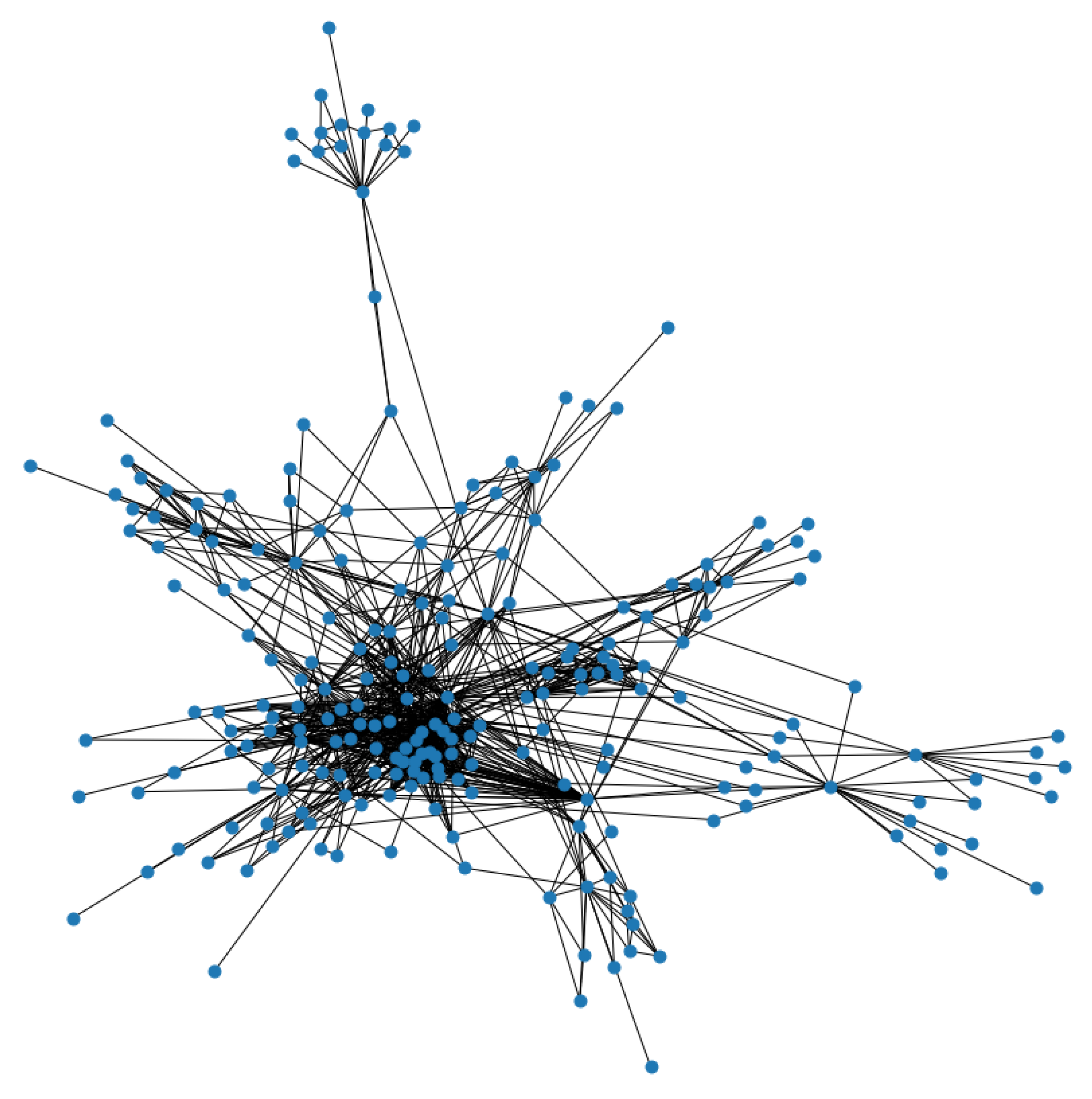
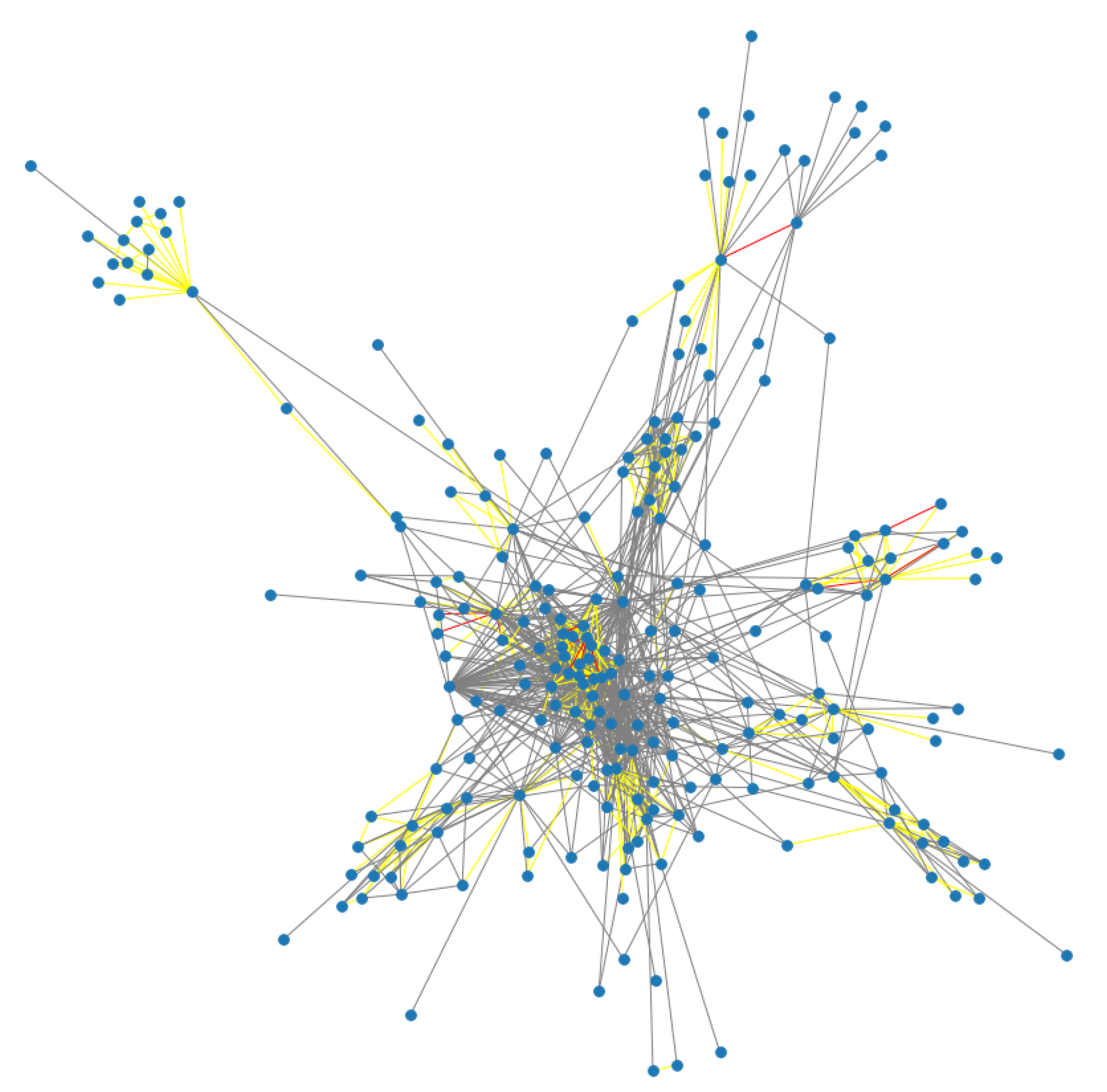
  • Data collection and network representation: The process begins by considering user profiles and extracting relevant features. These features are then used to create a graph that represents the social network.
  • Evaluation of user profiles: The next step involves evaluating the contribution of user profiles to the overall strength of the relationship. Various metrics and criteria are employed to assess the level of engagement.
  • Categorization of relationships: Based on the evaluated strength, the relationships are categorized into different levels or groups. This categorization provides insights into the varying degrees of engagement among users.
  • Presentation of statistical results: The study concludes by presenting statistical results and analyses related to the categorized relationships. These findings contribute to a deeper understanding of user engagement and the dynamics within the social network.
In summary, this paper employs a systematic approach that involves data collection, evaluation of user profiles, categorization of relationships, and statistical analysis to uncover the degree of user engagement based on the strength of their connections.
To determine the strength of the connections between two members, similarity features are considered, which encompass several aspects:
  • Common or close locations: The proximity or similarity of the locations associated with the user profiles is taken into account.
  • Similar scale in the number of friends: The comparison of the number of friends or connections between two user profiles helps gauge the similarity of their social network size.
  • Similar frequency of posts: The frequency at which users post on the platform is examined to identify similarities or patterns in their activity.
  • Interaction criteria: Various interaction metrics are considered, including friendship and follow relationships, as well as user mentions and retweets. These interactions indicate the level of engagement and connection between users.
By analyzing these similarity features, a score is derived for each edge, reflecting the strength of the connection between two members. The score is calculated based on the contribution of each feature, which may vary in terms of importance or weight. This scoring mechanism enables the categorization of relationships according to the calculated scores, providing insights into the varying strengths of connections within the social network.

4.2. Metrics

In the proposed method, two categories of metrics are utilized to calculate the score of each edge: similarity metrics and interaction metrics.
The similarity metrics focus on the popularity and characteristics of user accounts. These metrics include the number of followers and friends, which reflect the level of popularity and connectivity of an account. The number of tweets posted by each user is also considered, indicating their level of activity on the platform. Additionally, the geographic location of users is taken into account as a criterion of similarity. Users who are geographically closer are more likely to have a connection or friendship [19,24].
The interaction metrics capture the engagement and interaction between users. The mutual friendship condition is a crucial metric as it signifies a bidirectional connection, indicating a strong relationship between two users. The “following” feature is also considered, as it implies an interest in actively following the activities of another user on the social network. Mentions and replies in tweets are considered interaction features, indicating direct engagement and communication between users. Lastly, the exchange of messages, specifically the authorization from both sides to send and receive private messages, is included as a metric of interaction.
By incorporating these similarity and interaction metrics, the proposed method comprehensively captures various aspects of user engagement and connection on the social network, ultimately contributing to the calculation of the score for each edge.

4.3. Calculation of Connection Scores

The score of each edge is determined by considering the similarity and interaction metrics discussed above. The calculation process involves examining the set of collected edges and evaluating each metric based on specific conditions. The scores for the metrics are then summed up to obtain a final score for each edge.
The scores range from 0 to 10, where a score of 0 indicates no similarity or interaction between the profiles, while a score of 10 represents complete similarity and interaction.
However, not all metrics carry equal weight in determining the strength of a connection. Different weights are assigned to each metric to reflect their relative importance. The assigned weights for the metrics are presented in Table 1.
These weights reflect the relative importance of each metric in determining the strength of the user connections. By incorporating these weights into the scoring calculation, the proposed method can effectively capture the contribution of different metrics in evaluating the strength of relationships in the social network.
The selection of weights for user connection features is a crucial aspect of our analysis. These weights determine the relative importance of different user interactions, such as retweets, replies, and mentions. While we have chosen specific weights based on established research and prior knowledge, it is important to acknowledge that different weight configurations can yield varying results and potentially introduce biases. In this paper, we aim to explore the implications of different weight configurations theoretically, considering the impact on clustering outcomes and the interpretation of user engagement patterns.
The weights assigned to each metric reflect their relative importance in determining the strength of user connections. Specifically, features such as friend count and status count are given a weight of 1, indicating their moderate contribution to the strength of the connection. The location metric, on the other hand, is assigned a weight of 2, highlighting the significance of geographical proximity in fostering stronger connections.
The metric of mutual friendship is assigned the highest weight of 3, emphasizing the importance of bidirectional connections in indicating a strong relationship. This captures the idea that a mutual friendship indicates a deeper level of connection compared to a one-sided friendship. Reciprocity in the following is considered a powerful metric and is assigned a weight of 1. It signifies that both parties have expressed interest in connecting with each other, indicating a strong connection between them.
Mentions and replies, with weights of 1.5 , indicate a significant level of interaction between users. This interaction suggests a level of intimacy and engagement that goes beyond neutral or superficial connections. Lastly, both “following” and direct messages are assigned a weight of 1, denoting their contribution to the overall strength of the connection, but to a lesser extent compared to other metrics.
By assigning these weights, the proposed method takes into account the varying degrees of importance of different metrics in determining the strength of user connections, allowing for a more accurate assessment of relationship strength in the social network.
In the proposed method, the weights assigned to each metric are represented as elements of a weight vector, W = [ w 1 , w 2 , w 3 , w 4 , w 5 , w 6 , w 7 , w 8 ] . Similarly, the features of each edge are collected into a feature vector, V = [ v 1 , v 2 , v 3 , v 4 , v 5 , v 6 , v 7 , v 8 ] .
To calculate the total score for an edge connecting user A to user B in a specific Twitter subgraph, the weight vector W is multiplied element-wise with the feature vector V, and the resulting values are summed. Mathematically, the score is computed as follows:
Score ( A , B ) = i = 1 8 w i · v i
After calculating the scores for each pair of edges using Equation (1), the scores need to be normalized in order to categorize the edges effectively. The normalization process ensures that the scores are scaled to a range between 0 and 10.
The normalization formula is given by Equation (2), where N o r m S c o r e ( A , B ) represents the normalized score for the edge connecting node A to node B. The numerator in the equation represents the subtraction of the minimum score value from each calculated score, while the denominator represents the range between the maximum and minimum score values. The resulting value is then multiplied by 10 to scale it to the desired range.
Norm Score ( A , B ) = S c o r e ( A , B ) m i n ( S c o r e ( A , B ) ) m a x ( S c o r e ( A , B ) m i n ( S c o r e ( A , B ) · 10
By applying this normalization equation, the scores of each edge will be transformed to a standardized range of values between 0 and 10. This normalization step enables the categorization of the edges based on their normalized scores, providing a clearer representation of the strength of the connections within the social network.

4.4. Edges Categorization

The edges are categorized based on the strength of their scores obtained from the previous calculations. Five classes are defined to represent different levels of connection strength. The categories are determined based on the intervals in which the scores fall.
The edge categorization classes and their corresponding score intervals are as follows:
  • Indifferent [0, 2].
  • Weak (3, 4].
  • Medium (5, 6].
  • Strong (7, 8].
  • Very strong (9, 10].
Higher scores correspond to stronger connections, and the maximum score achievable is 10. This score indicates maximum similarity and interaction between the connected profiles, where all metrics contribute optimally. The choice of five classes for categorization is based on the recommendations of researchers from various scientific disciplines and ensures a suitable distribution of connections among Twitter users.

5. Implementation

To construct the Twitter subgraph for our study, we adhered to the limitations imposed by the Twitter API. The data collection process took place within a one-month time interval, specifically from 1 June to 30 June 2022. For sampling tweets related to our study, a topic-based approach was employed. We focused on tweets that contained the keyword #bigdata, which represents a discussion topic of significant interest in both scientific and business contexts. This hashtag was chosen because it exhibited sparse but consistent activity over time.
The dataset construction involved a two-step process. Firstly, we harvested tweets that matched the specified topic, collecting a total of 13,128 tweets. Secondly, we queried Twitter to retrieve the followers and friends for each active user identified in the first step. This process resulted in a dataset consisting of 1354 user accounts from 115 different locations, with a total of 253,655 followers. By following this methodology, we aimed to create a representative Twitter subgraph that captures the dynamics and relationships among users discussing the topic of big data during the specified time period.
The following Figure 1 illustrates a social media graph and specifically the minimum cohesive graph of the particular users’ network where the nodes without edges were removed. There were such edgeless nodes as access to the lists of some user profiles was prohibited. The blue dots represent Twitter profiles and the edges represent the “follow” connection between two users. As expected, the network appears to have much denser relationships internally, i.e., in its center, since the starting node constitutes the core of the network.
After removing the users without any edges in the dataset, we performed the experiments using a total of 1150 users. This step was taken to ensure that the analysis and results were based on a meaningful subset of users with established connections within the social network. By focusing on users with edges, we aimed to capture and analyze the patterns of engagement and interactions within the network more accurately.
Table 2 provides the distribution of users based on the number of friends they have on Twitter. A significant proportion, approximately 22% of users, have between 0 and 100 friends. The largest group, comprising around 35% of users, falls into the range of 101 to 500 friends. Another notable segment, approximately 23% of users, has between 501 and 1000 friends. A smaller portion, around 11% of users, falls into the range of 1001 to 5000 friends. Lastly, approximately 9% of users have a substantial number of friends, exceeding 5000.
This distribution provides insights into the connectivity patterns of users in the analyzed Twitter network. It suggests that a significant portion of users have a moderate number of friends, while a smaller percentage of users have a larger number of friends.
The distribution of users based on the number of followers they have on Twitter can be summarized in Table 3. Approximately 12% of users have between 0 and 100 followers, while another 11% have between 101 and 500 followers. A smaller proportion, around 9% of users, fall into the range of 501 to 1000 followers. The segment of users with a larger following includes approximately 13% with 1001 to 5000 followers. The majority of users, comprising approximately 55%, have a substantial number of followers, exceeding 5000. This distribution highlights the varying influence and reach levels within the analyzed Twitter network, with a significant percentage of users having a considerable number of followers while others have a more limited audience.
The distribution of users based on the number of tweets they have posted on Twitter is presented in Table 4. The percentages closely resemble the distribution in Table 3. Approximately 6% of users have posted between 0 and 100 tweets, while around 9% have posted between 101 and 500 tweets. Similarly, about 10% of users fall into the range of 501 to 1000 tweets, and a larger proportion, approximately 25%, have posted between 1001 and 5000 tweets. The majority, comprising about 50% of users, have posted over 5000 tweets. This distribution reflects the varying levels of activity and engagement among users, with some being more active and prolific in sharing content on the platform compared to others.
The analysis of the tables reveals several trends within the dataset. Firstly, there are a significant number of popular users with a high number of friends and followers. This indicates that these users have amassed a considerable network and attracted a large audience on Twitter. Secondly, the high percentages of users who have posted thousands of tweets indicate a high level of activity and engagement within the dataset. These users are actively sharing content and interacting with others on the platform. The combination of a large number of friends, followers, and a substantial tweet count suggests that the dataset includes influential and active users who play an important role within the Twitter network.

6. Evaluation

6.1. Analysis of User Relationship Strength

Table 5 provides insights into the contribution of each metric to the overall score of the edges. The metrics with the highest scores are ‘direct message’ and ‘mutual friendship’, accounting for 35.5 % and 33 % of the overall score, respectively. Following closely are the three similarity metrics—friends count, location, and statuses count—contributing 9.5 % , 9 % , and 7.5 % to the score, respectively. On the other hand, the remaining three interaction metrics, namely reply, mention, and following, have lower contributions, each accounting for less than 3 % of the overall score.
This analysis provides valuable information about the importance of each metric in determining the strength of the connections between users. The high contribution of ‘direct message’ and ‘mutual friendship’ suggests that these metrics play a significant role in establishing strong connections. The similarity metrics also contribute significantly, indicating that users with similar friend counts, locations, and posting activity are more likely to have stronger connections. Meanwhile, the lower contributions of Reply, Mention, and Following metrics suggest that these interactions have less impact on the overall strength of the connections.
By understanding the percentage contribution of each metric, we can gain insights into the factors that influence the categorization and strength of the edges in the Twitter subgraph.
The categorization of the edges into five classes based on their scores provides an overview of the distribution of connection strengths in the Twitter subgraph. Table 6 displays the percentages of edges in each class.
The majority of edges fall into the indifferent class, constituting 50.7 % of the total. This suggests that a significant portion of connections in the subgraph exhibit low similarity and interaction scores. The weak class represents 29.65 % of the edges, indicating slightly stronger connections compared to the Indifferent class. The medium class comprises 15.35 % of the edges, indicating connections with moderate strength. This class may represent connections with a balanced level of similarity and interaction. The strong class accounts for 3.75 % of the edges, indicating a higher level of connection strength. The very strong class has the smallest percentage, with only 0.55 % of the edges falling into this category. This class represents the strongest connections in the subgraph, indicating a high level of similarity and interaction between users. It is expected for the very strong class to have a small percentage, as such strong ties are typically formed among a limited number of users.
The categorization of edges into these classes provides valuable insights into the distribution of connection strengths within the Twitter subgraph, highlighting the prevalence of weaker and more indifferent connections while also identifying a smaller proportion of stronger ties.
Figure 2 is the same as Figure 1 but with additional color on the edges according to the above categories. Specifically, very strong and strong edges are illustrated in red, medium and weak edges are illustrated in yellow, and indifferent edges are illustrated in gray. The presence of colored areas in contrast to others suggests the formation of smaller sub-networks or user groups within the larger social network. These sub-networks consist of strongly connected users who interact with each other in a more detailed and intense manner. The color-coded edges provide a visual representation of the varying levels of connection strength between users in the graph, highlighting the presence of distinct groups or clusters within the overall network structure.
The density value of 0.04 indicates that the graph has a relatively low number of connections compared to the maximum possible number of connections. A density of 1 would mean that every pair of nodes in the graph is connected by an edge. In this case, the density of 0.04 suggests that only a small fraction of possible connections is present in the graph, indicating a sparse network.
The diameter of the graph being 4 means that the longest shortest path between any two vertices in the graph requires traversing a maximum of 4 vertices. In other words, it takes at most four steps to go from one node to another, excluding paths that involve looping. The diameter is a measure of the graph’s overall “reach” or “distance” between nodes. A smaller diameter indicates that nodes in the graph are relatively closer to each other in terms of their connectivity.
While direct comparisons to other social networks are not available in this study, it is important to note that the values of density and diameter can vary significantly across different types of social networks. Social networks exhibit diverse structures and user behaviors, influenced by factors such as the platform’s design, user demographics, and the purpose of the network.
The observation of strong connections (red edges) in Figure 2 reveals an interesting pattern among users who have a higher overall engagement. It is noteworthy that these users tend to have fewer friends and belong to smaller groups. This raises the question of whether users with a larger number of friends exhibit higher overall engagement but with each individual edge having a lower score. This phenomenon can be attributed to the concept of social capital, where users with fewer friends often have more focused and stronger connections, resulting in higher individual edge scores. Conversely, users with a larger number of friends may have more diverse connections and interactions, leading to lower individual edge scores but potentially higher overall engagement. It is important to recognize that these observations are context-dependent and may vary based on the specific characteristics of the social network and user behavior. Further research and analysis are necessary to gain a more comprehensive understanding of the relationship between the number of friends, individual edge scores, and overall engagement in the given network.
Overall, the density and diameter values provide insights into the structure and connectivity of the graph, indicating the level of interconnections and the maximum distance between nodes in the network.

6.2. Clustering Algorithms Comparison

In this subsection, the graphical representation of the results regarding the seven clustering algorithms is presented. Specifically, Figure 3 illustrates the results of k-means, bisecting k-means, DBSCAN, OPTICS, the Gaussian mixture model, hierarchical clustering, and spectral clustering.
In the analysis of the clustering algorithms, it was found that DBSCAN and OPTICS algorithms resulted in six and seven clusters, respectively, without requiring a predetermined number of clusters. However, the OPTICS algorithm encountered difficulty in classifying a significant amount of data, leading to a category of unspecified data, as shown by the blue color in Figure 3d. This behavior was expected due to the algorithm’s limitation in determining clusters for spatial data. It is evident that the OPTICS algorithm would benefit from improved clustering performance for the given data.
In the analysis of the expectation–maximization and spectral clustering algorithms, different techniques were employed to determine the number of components and clusters. However, for the present work, the number of clusters obtained from the silhouette and elbow methods for k-means was considered. Regarding the DBSCAN algorithm, Figure 3c shows that small amounts of data were left in the undefined category. Additionally, a large cluster was formed, encompassing a significant portion of the data, along with seven smaller clusters, some of which contained only a single data point. This behavior could be attributed to the parameter values chosen for ϵ and m i n P t s , which were set to 5 and 6, respectively.
Similarly, the spectral clustering algorithm resulted in a large cluster containing a significant amount of data, along with seven smaller clusters, each consisting of only one data point, as depicted in Figure 3g. This discrepancy can be attributed to the chosen number of clusters, which was set to 8, similar to the other algorithms, but may not have been suitable for this specific algorithm. Overall, the analysis reveals that the DBSCAN and spectral clustering algorithms did not produce satisfactory results, with deviations from the expected number of clusters and suboptimal clustering patterns.
The k-means and bisecting k-means algorithms are effective in spatial data geometries as they cluster the data around specific points, such as the centroids of the clusters. This can be observed in Figure 3a,b. These algorithms are well-suited for situations where the data points are spatially distributed and can be clearly separated into distinct clusters. In contrast, the expectation–maximization algorithm, which relies on the Gaussian mixture model, converges the clusters around the Gaussian surfaces calculated by the model. This makes it more suitable for flat data geometries where the data points follow a Gaussian distribution. In such cases, the expectation–maximization algorithm can effectively estimate the parameters of the Gaussian distributions and cluster the data accordingly.
The choice of algorithm should be based on the nature of the data and the underlying distribution. k-means and bisecting k-means are preferable for spatial data, while expectation–maximization is better suited for data with a flat geometry and Gaussian distribution.
Based on the patterns observed in the grouped data, it can be claimed that the k-means, bisecting k-means, expectation–maximization, and hierarchical clustering algorithms produced the best results. These algorithms demonstrated satisfactory clustering performance and effectively captured the underlying patterns in the data. On the other hand, the remaining three algorithms (DBSCAN, OPTICS, and spectral clustering) did not perform as well and did not produce satisfactory results. These algorithms either failed to classify a significant amount of data into clusters or created clusters with only a few data points, indicating suboptimal clustering performance.

7. Discussion

7.1. Insights into User Relationship Dynamics

The experimental study has provided valuable insights into the distribution and characteristics of the Twitter subgraph. The analysis of the metrics’ contribution to the edge scores highlights the importance of various factors in determining the strength of connections between users. The metrics related to the number of friends, posts, and locations play a significant role, indicating the importance of these factors in establishing relationships on social media.
To further explore the significance of location in determining connection strength, it is worth noting that many users do not disclose their location on their profiles. However, the location similarity metric may have an even more influential role if more users provided this information. Additionally, considering that users may have interactions on multiple social media platforms, the analysis could be extended to incorporate data from other platforms to capture a more comprehensive view of user interactions.
Another intriguing finding is the identification of smaller strong sub-networks within the larger network. These sub-networks, represented by the colored edge regions in Figure 2, indicate the presence of tightly connected user groups. A further investigation of these sub-networks could provide insights into the dynamics, interactions, and potential community structures within these groups. By extracting and studying these sub-networks separately, it would be possible to explore their specific characteristics and analyze their robustness in more detail.
Table 1 presents the weights assigned to each metric category and its corresponding metrics for evaluating the strength of user connections. These weights were determined based on their perceived significance in capturing the strength of user relationships in the Twitter network. However, in Table 5, we provide an analysis of the overall score contribution percentage of each metric category and metric based on the experimental results. It is important to note that the contribution percentages in Table 5 may differ from the assigned weights in Table 1. This discrepancy arises due to the influence of the specific dataset and characteristics of the Twitter network used in our experiments. The experimental results reveal variations in the relative importance of different metrics, suggesting that the assigned weights in Table 1 may not fully capture the true impact of each metric on the overall user connection strength.

7.2. Interpretation of Clustering Results

It is important to note that different algorithms have different strengths and weaknesses, and their performance can vary depending on the dataset and the specific problem at hand. In this case, the mentioned algorithms were compared based on the given dataset and the desired number of clusters. It is also worth mentioning that no single algorithm achieved the exact same clustering result as another algorithm. This highlights the fact that different clustering algorithms may produce different cluster assignments, and the choice of the algorithm should be based on the specific requirements and characteristics of the data.
Moreover, it is crucial to acknowledge that the quality of the results could be further improved with higher-quality data and algorithms that are specifically tailored to the problem at hand. The efficiency of the algorithms in relation to the specific problem is also an important consideration. Different clustering algorithms may have different assumptions, requirements, and limitations. Choosing the most appropriate algorithm that aligns with the characteristics of the data and the problem can significantly improve the quality of the clustering results.
Furthermore, preprocessing steps such as data cleaning, feature selection or extraction, and normalization can also contribute to improving the quality of the data and consequently enhance the performance of the clustering algorithms.
It is essential to note that clustering is an unsupervised learning task, and the quality of the results depends on various factors, including the nature of the data, the algorithm used, and the specific problem requirements. Therefore, careful consideration of these factors and continuous evaluation and refinement of the clustering approach can lead to better results.
The credibility of the Twitter data used in this study warrants discussion, as users on social media platforms can potentially provide false or inaccurate information on their profiles. While efforts were made to collect data from active and verified users, it is important to acknowledge that the possibility of misleading or unreliable information cannot be completely eliminated. Additionally, the limited data collected in this study may not fully represent the entire Twitter user population. The sample size of users included in the analysis was determined based on the availability of user edges and met certain criteria. Therefore, caution should be exercised in generalizing the findings to the entire Twitter social network. Future research could consider exploring larger and more diverse datasets to further examine the credibility and representativeness of social network data.
Overall, the results of this study highlight the complexity and diversity of social media networks and provide a foundation for further research and analysis in understanding user interactions, community structures, and the dynamics of online social networks.

8. Conclusions and Future Work

In conclusion, this study employed graph mining techniques to analyze user engagement levels and the strength of connections in a social network. By leveraging clustering algorithms, we gained valuable insights into the formation and behavior of node groups within the network. The findings highlight the significance of examining both individual and group behavior, shedding light on the dynamics of social networks. The integration of real-time and historical data not only provides a comprehensive understanding of user relationships but also offers the potential to predict future connections. This interdisciplinary research, drawing from computer science, psychology, and sociology, contributes to a deeper understanding of user behavior and its profound impact on the structure and evolution of social networks.
It is important to acknowledge that the Twitter data collected in this study represent a specific study area that encompasses users from diverse backgrounds and geographical locations. Although a specific study area was not explicitly defined, the data collection process aimed to include a wide range of users to ensure diversity and capture a variety of social connections. Therefore, the findings of this study should be interpreted within the context of the specific study area, recognizing that they may not directly generalize to other social networks or geographic regions.
To gain a more comprehensive understanding of social network dynamics, future research could explore the potential variations in user connections across different study areas. Comparing the findings of this study with similar studies conducted in different regions or on different social platforms can provide valuable insights into the generalizability of the observed patterns. Additionally, investigating the impacts of cultural differences, language preferences, and regional dynamics on social connections can further enhance our understanding of the context-specific nature of social networks.
For future work, it is suggested to explore variations and combinations of the proposed methods to improve their performance [37,38]. The implementation of parallel computing techniques and streaming analytics technologies can enable the creation of a near-real-time user relationship analysis system. This system would be capable of identifying changes in relationships over time and potentially learn and predict network alterations. Additionally, integrating algorithms to predict the likelihood of connections between users could further enhance the capabilities of the system.
Continued research and development in this area can contribute to a deeper understanding of user engagement in social networks and facilitate the development of more advanced and effective analysis and prediction techniques.

Author Contributions

Conceptualization, A.K., I.K. and A.M.; Methodology, A.K., I.K. and A.M.; Data curation, A.K., I.K. and A.M.; Writing—original draft, A.K., I.K. and A.M.; Writing—review & editing, A.K., I.K. and A.M. All authors have read and agreed to the published version of the manuscript.

Funding

This research received no external funding.

Data Availability Statement

All data were presented in the main text.

Conflicts of Interest

The authors declare no conflict of interest.

References

  1. Kafeza, E.; Kanavos, A.; Makris, C.; Pispirigos, G.; Vikatos, P. T-PCCE: Twitter Personality based Communicative Communities Extraction System for Big Data. IEEE Trans. Knowl. Data Eng. 2020, 32, 1625–1638. [Google Scholar] [CrossRef]
  2. Kanavos, A.; Drakopoulos, G.; Tsakalidis, A.K. Graph Community Discovery Algorithms in Neo4j with a Regularization-based Evaluation Metric. In Proceedings of the 13th International Conference on Web Information Systems and Technologies (WEBIST), Porto, Portugal, 25–27 April 2017; pp. 403–410. [Google Scholar]
  3. Noordhuis, P.; Heijkoop, M.; Lazovik, A. Mining Twitter in the Cloud: A Case Study. In Proceedings of the IEEE International Conference on Cloud Computing (CLOUD), Miami, FL, USA, 5–10 July 2010; pp. 107–114. [Google Scholar]
  4. Lin, M.F.G.; Hoffman, E.S.; Borengasser, C. Is Social Media Too Social for Class? A Case Study of Twitter Use. TechTrends 2013, 57, 39–45. [Google Scholar] [CrossRef]
  5. Tripathy, B.K.; Mitra, A. An Algorithm to Achieve k-Anonymity and l-Diversity Anonymisation in Social Networks. In Proceedings of the 4th International Conference on Computational Aspects of Social Networks (CASoN), Sao Carlos, Brazil, 21–23 November 2012; pp. 126–131. [Google Scholar]
  6. Wasserman, S.; Faust, K. Social Network Analysis: Methods and Applications; Cambridge University Press: Cambridge, UK, 1994. [Google Scholar]
  7. Drakopoulos, G.; Gourgaris, P.; Kanavos, A. Graph Communities in Neo4j. Evol. Syst. 2020, 11, 397–407. [Google Scholar] [CrossRef]
  8. Candon, P. Twitter: Social Communication in the Twitter Era. New Media Soc. 2019, 21, 146144481983198. [Google Scholar] [CrossRef]
  9. Quercia, D.; Kosinski, M.; Stillwell, D.; Crowcroft, J. Our Twitter Profiles, Our Selves: Predicting Personality with Twitter. In Proceedings of the 3rd International IEEE Conference on Privacy, Security, Risk and Trust (PASSAT) and 3rd International IEEE Conference on Social Computing (SocialCom), Boston, MA, USA, 9–11 October 2011; pp. 180–185. [Google Scholar]
  10. Christakis, N.A.; Fowler, J.H. Connected: The Surprising Power of Our Social Networks and How They Shape Our Lives; Little, Brown and Company: Boston, MA, USA, 2009. [Google Scholar]
  11. Kalogeropoulos, N.R.; Doukas, I.; Makris, C.; Kanavos, A. A Graph-Based Extension for the Set-Based Model Implementing Algorithms Based on Important Nodes. In Proceedings of the 16th International Conference on Artificial Intelligence Applications and Innovations (AIAI), Halkidiki, Greece, 5–7 June 2020; pp. 143–154. [Google Scholar]
  12. Dhillon, I.S.; Guan, Y.; Kulis, B. A Fast Kernel-based Multilevel Algorithm for Graph Clustering. In Proceedings of the 11th ACM SIGKDD International Conference on Knowledge Discovery and Data Mining, Chicago, IL, USA, 21–24 August 2005; pp. 629–634. [Google Scholar]
  13. Ozaki, T.; Ohkawa, T. Mining Correlated Subgraphs in Graph Databases. In Proceedings of the 12th Pacific-Asia Conference on Advances in Knowledge Discovery and Data Mining (PAKDD), Osaka, Japan, 20–23 May 2008; pp. 272–283. [Google Scholar]
  14. Le, T.V.; Kulikowski, C.A.; Muchnik, I.B. Coring Method for Clustering a Graph. In Proceedings of the 19th International Conference on Pattern Recognition (ICPR), Tampa, FL, USA, 8–11 December 2008; pp. 1–4. [Google Scholar]
  15. Kraus, J.M.; Palm, G.; Kestler, H. On the Robustness of Semi-Supervised Hierarchical Graph Clustering in Functional Genomics. In Proceedings of the 5th International Workshop on Mining and Learning with Graphs, Florence, Italy, 1–3 August 2007; pp. 147–150. [Google Scholar]
  16. Wilson, C.; Boe, B.; Sala, A.; Puttaswamy, K.P.N.; Zhao, B.Y. User Interactions in Social Networks and their Implications. In Proceedings of the EuroSys, Nuremberg, Germany, 1–3 April 2009; pp. 205–218. [Google Scholar]
  17. Kim, J.; Lee, E.; Choi, J.; Bae, Y.; Ko, M.; Kim, P. Monitoring Social Relationship among Twitter Users by using NodeXL. In Proceedings of the Research in Adaptive and Convergent Systems (RACS), Montreal, QC, Canada, 1–4 October 2013; pp. 107–110. [Google Scholar]
  18. Davis, C.A., Jr.; Pappa, G.L.; de Oliveira, D.R.R.; de Lima Arcanjo, F. Inferring the Location of Twitter Messages Based on User Relationships. Trans. GIS 2011, 15, 735–751. [Google Scholar]
  19. Priedhorsky, R.; Culotta, A.; Valle, S.Y.D. Inferring the Origin Locations of Tweets with Quantitative Confidence. In Proceedings of the Computer Supported Cooperative Work (CSCW), Baltimore, MD, USA, 15–19 February 2014; pp. 1523–1536. [Google Scholar]
  20. Xiang, R.; Neville, J.; Rogati, M. Modeling Relationship Strength in Online Social Networks. In Proceedings of the 19th International Conference on World Wide Web (WWW), Raleigh, NC, USA, 26–30 April 2010; pp. 981–990. [Google Scholar]
  21. McPherson, M.; Smith-Lovin, L.; Cook, J.M. Birds of a Feather: Homophily in Social Networks. Annu. Rev. Sociol. 2001, 27, 415–444. [Google Scholar] [CrossRef] [Green Version]
  22. Dehghani, M.; Johnson, K.; Hoover, J.; Sagi, E.; Garten, J.; Parmar, N.J.; Vaisey, S.; Iliev, R.; Graham, J. Purity Homophily in Social Networks. J. Exp. Psychol. Gen. 2016, 145, 366. [Google Scholar] [CrossRef] [PubMed]
  23. Liben-Nowell, D.; Kleinberg, J.M. The Link-Prediction Problem for Social Networks. J. Am. Soc. Inf. Sci. Technol. (JASIST) 2007, 58, 1019–1031. [Google Scholar] [CrossRef] [Green Version]
  24. Dougnon, R.Y.; Fournier-Viger, P.; Nkambou, R. Inferring User Profiles in Online Social Networks Using a Partial Social Graph. In Proceedings of the 28th Canadian Conference on Artificial Intelligence (AI), Halifax, NS, Canada, 2–5 June 2015; Volume 9091, pp. 84–99. [Google Scholar]
  25. Rong, X. Word2vec Parameter Learning Explained. arXiv 2014, arXiv:1411.2738. [Google Scholar]
  26. Likas, A.; Vlassis, N.; Verbeek, J.J. The Global k-means Clustering Algorithm. Pattern Recognit. 2003, 36, 451–461. [Google Scholar] [CrossRef] [Green Version]
  27. Savaresi, S.M.; Boley, D. On the Performance of Bisecting K-means and PDDP. In Proceedings of the 1st SIAM International Conference on Data Mining (SDM), Chicago, IL, USA, 5–7 April 2001; pp. 1–14. [Google Scholar]
  28. Schubert, E.; Sander, J.; Ester, M.; Kriegel, H.; Xu, X. DBSCAN Revisited, Revisited: Why and How You Should (Still) Use DBSCAN. ACM Trans. Database Syst. 2017, 42, 19:1–19:21. [Google Scholar] [CrossRef]
  29. Ankerst, M.; Breunig, M.M.; Kriegel, H.; Sander, J. OPTICS: Ordering Points To Identify the Clustering Structure. In Proceedings of the ACM SIGMOD International Conference on Management of Data, Philadelphia, PA, USA, 1–3 June 1999; pp. 49–60. [Google Scholar]
  30. Reynolds, D.A. Gaussian Mixture Models. In Encyclopedia of Biometrics; Springer: Cham, Switzerland, 2009; pp. 659–663. [Google Scholar]
  31. Moon, T.K. The Expectation-Maximization Algorithm. IEEE Signal Process. Mag. 1996, 13, 47–60. [Google Scholar] [CrossRef]
  32. Nielsen, F. Hierarchical Clustering. In Introduction to HPC with MPI for Data Science; Springer: Cham, Switzerland, 2016; pp. 195–211. [Google Scholar]
  33. Ng, A.Y.; Jordan, M.I.; Weiss, Y. On Spectral Clustering: Analysis and an Algorithm. In Proceedings of the Advances in Neural Information Processing Systems 14 (NIPS), Vancouver, BC, Canada, 3–8 December 2001; pp. 849–856. [Google Scholar]
  34. Kanavos, A.; Livieris, I.E. Fuzzy Information Diffusion in Twitter by Considering User’s Influence. Int. J. Artif. Intell. Tools 2020, 29, 2040003:1–2040003:22. [Google Scholar] [CrossRef]
  35. Zamparas, V.; Kanavos, A.; Makris, C. Real Time Analytics for Measuring User Influence on Twitter. In Proceedings of the 27th IEEE International Conference on Tools with Artificial Intelligence (ICTAI), Vietri sul Mare, Italy, 9–11 November 2015; pp. 591–597. [Google Scholar]
  36. Drakopoulos, G.; Kanavos, A.; Paximadis, K.; Ilias, A.; Makris, C.; Mylonas, P. Computing Massive Trust Analytics for Twitter using Apache Spark with Account Self-assessment. In Proceedings of the 16th International Conference on Web Information Systems and Technologies (WEBIST), Virtual Event, 3–5 November 2020; pp. 403–414. [Google Scholar]
  37. Drakopoulos, G.; Kanavos, A.; Tsakalidis, A.K. Evaluating Twitter Influence Ranking with System Theory. In Proceedings of the 12th International Conference on Web Information Systems and Technologies (WEBIST), Rome, Italy, 23–25 April 2016; pp. 113–120. [Google Scholar]
  38. Kyriazidou, I.; Drakopoulos, G.; Kanavos, A.; Makris, C.; Mylonas, P. Towards Predicting Mentions to Verified Twitter Accounts: Building Prediction Models over MongoDB with Keras. In Proceedings of the 15th International Conference on Web Information Systems and Technologies (WEBIST), Vienna, Austria, 18–20 September 2019; pp. 25–33. [Google Scholar]
Figure 1. Initial Network.
Computers 12 00124 g001
Figure 2. Final network.
Computers 12 00124 g002
Figure 3. Clustering Algorithms.
Computers 12 00124 g003
Table 1. Weights per Metric.
Metric CategoryMetricSymbolWeight
SimilarityFriends Count u 1 1
Location u 2 2
Statuses Count u 3 1
InteractionDirect Message u 4 1
Following u 5 1
Mention u 6 1.5
Mutual Friendship u 7 3
Reply u 8 1.5
Table 2. Percentage of users based on number of friends.
Number of FriendsPercentage of Users
0–10022
101–50035
501–100023
1001–500011
over 50009
Table 3. Percentage of users based on number of followers.
Number of FollowersPercentage of Users
0–10012
101–50011
501–10009
1001–500013
over 500055
Table 4. Percentage of users based on number of tweets.
Number of TweetsPercentage of Users
0–1006
101–5009
501–100010
1001–500025
over 500050
Table 5. Percentage contribution of the overall score by edges.
Metric CategoryMetricOverall Score Contribution
SimilarityFriends Count9.5
Location9
Statuses Count7.5
InteractionDirect Message35.5
Following1
Mention1.5
Mutual Friendship33
Reply3
Table 6. Percentages of edges.
ClassesEdges
Very Strong0.55
Strong3.75
Medium15.35
Weak29.65
Indifferent50.7
Disclaimer/Publisher’s Note: The statements, opinions and data contained in all publications are solely those of the individual author(s) and contributor(s) and not of MDPI and/or the editor(s). MDPI and/or the editor(s) disclaim responsibility for any injury to people or property resulting from any ideas, methods, instructions or products referred to in the content.

