


Disparity of Density in the Age of Mobility: Analysis by Opinion Formation Model
Faculty of International Tourism, Hannan University, Matsubara 580-0032, Japan
Computers 2023, 12(5), 94; https://doi.org/10.3390/computers12050094
Submission received: 31 March 2023
/
Revised: 25 April 2023
/
Accepted: 26 April 2023
/
Published: 1 May 2023
(This article belongs to the Special Issue Computational Modeling of Social Processes and Social Networks)
Abstract
:High mobility has promoted the concentration of people’s aggregation in urban areas. As people pursue areas with higher density, gentrification and sprawl become more serious. Disadvantaged people are then pushed out of urban centers. Conversely, as mobility increases, the disadvantaged may also migrate in pursuit of their desired density. As a result, disparities relative to density and housing may shrink. Hence, migration is a complex system. Understanding the effects of migration on disparities intuitively is difficult. This study explored the effects of mobility on disparity using an agent-based model of opinion formation. We find that as mobility increases, disparities between agents in density and diversity widen, but as mobility increases further, the disparities shrink, and then widen again. Our results present possibilities for a just city in the age of mobility.
1. Introduction
Mobility is a new paradigm that can be used to understand the changing world [1,2]. The increasing convenience of transportation has changed people’s lives. People have enjoyed the development of cars, airplanes, and other modes of transportation, and of railways and roads. Many people now have access to such means of transportation. Hence, people now have the option to live and work wherever they choose and, hence, broaden their social relationships [3,4,5]. The distinction between work and leisure has become blurred. Owing to the development of tourism, people now travel greater distances with more frequency. Tourism has now become part of some people’s jobs and has changed their lifestyles [6,7]. The spread of information and communication technology (ICT) has also contributed to higher mobility. Owing to smartphones and social networking services, people can stay connected to their distant relatives and friends and obtain the information necessary for them to travel to their desired locations [8,9]. Social relationships through social networking services are critical not only in migration but also in tourism [10,11,12]. By contrast, as evidenced by war and environmental refugees, not all people migrate by choice. We need to be aware of the disparity between those who have the privilege to migrate and those who do not. For example, people with health problems and the poor are excluded not only from the use of private vehicles but also from public transport and ICTs. This negatively affects their mobility and, hence, the general well-being of the disadvantaged [13].
This study focuses on the concentration of people in urban areas caused by increased mobility. People tend to migrate to or visit urban areas in search of higher income and opportunities for jobs and leisure in both developed and developing countries [14,15,16,17,18,19,20]. As transportation and ICT become more widespread, concentration in urban areas will likely strengthen. People from a wider range of areas, both domestic and international, are more likely to be attracted to urban areas. However, capital investment in large cities is mainly aimed at attracting large corporations and tourists, and housing development has not caught up. We see gentrification in many urban areas where low-income residents are forced to live in poor housing conditions. In some cases, they are evicted because they cannot afford to live in the area [21,22,23,24,25,26]. Even if poor residents could live in gentrified areas, which attract multinational corporations and tourists, inequalities often increase. This is because financial and information workers earn high incomes, while unskilled service workers are placed in low-income situations [27,28]. The high densities of urban areas also cause problems such as crime [29,30]. While the wealthy can protect themselves from such risks by, for instance, living in condominiums, the poor have to endure not only poor living conditions but also deteriorating public safety. People with low incomes, illnesses, disabilities, or limited access to ICTs are forced into situations of poverty, isolation, and other disadvantages in urban areas built on the premise of high mobility. Even if the poor may reside in urban areas, stores and public transportation are less available in areas with high concentrations of poor people, making their lives more difficult [31,32,33]. Further globalization may lead to super-gentrification, wherein not only the poor but also the middle class will find living in urban areas difficult [34,35]. With justice in mind after COVID-19, disparities in urban areas should be corrected [36].
The rise in mobility does not only result in migration to urban areas. Migrations from urban to rural areas have also become easier. Owing to the natural beauty of rural areas, rural tourism remains popular. People are increasingly becoming attracted to such nature-rich rural areas. Owing to the blurring of the boundaries between tourism and migration, lifestyle migrants, who seek a more relaxed life in rural areas, may increase [37,38,39]. In the past, only global elites could freely select multiple areas for their residence and their jobs [40,41]. However, now, the number of digital nomads—people who work and live while traveling the globe—is increasing [42,43]. However, this way of life is not open to all people, and there may be disparities in peoples’ options to move to rural areas.
In summary, the push factor for migration is the cost of living associated with high density, and the pull factor is the density that people seek. Different people have different tolerance for density costs and different opinions about density, so the problem becomes a complex system. Furthermore, the migration of people, the resulting changes in density, and the disparities found therein are complex systems that interact with each other. Hence, these systems are difficult to understand intuitively. Responding to these issues, this study considers the relationship between mobility, density, and disparity using an agent-based model (ABM).
2. Theoretical Background
Many ABMs that tackle migration have been developed. These ABMs assume that agents seek economic opportunity or income. Agents are expected to gather in urban areas, where economic opportunities and incomes are more available [44,45,46,47]. This concentration of people in urban areas results in higher living costs (e.g., rent), which is associated with higher density. This may result in reinforced disparities in a residential location. Wealthier people can tolerate higher densities, while the poor are typically evicted to the periphery [48,49].
When people migrate, they do not necessarily do so to maximize economic opportunities. Some people move to a new area owing to certain features of the living environment (e.g., neighborhood, amenities, and level of public safety). People migrate to areas where they can walk or cycle to work, enjoy rich natural environments while doing the work they want, or raise their children comfortably. Some people aim to move to environments that were considered inferior but would allow them to meet a more diverse range of neighbors. Hence, ABMs that assume that people migrate based on preferences other than economic opportunity have also been developed. The models assume that agents make migration decisions based on their potential neighbors, ethnicities, jobs, or incomes. Moreover, agents are assumed to migrate based on other factors (e.g., housing prices, available transportation, commuting time to offices, and the potential networks available) [50,51,52,53,54,55,56,57].
Types of preferred living environments should vary among people. Population density can be considered an indicator that influences living conditions, including economic opportunities. Generally, in higher-density areas, residents are more likely to gain higher incomes, but they also incur higher living costs. In lower-density areas, residents often enjoy living environments of natural beauty. Different people have different ideas about the type of density they are looking for. People could be assumed to seek their ideal population density. Their opinions about density will change in their interactions with others and with the environment. Some people seek to maximize economic opportunities, while others value other aspects of the living environment. Disparities among people may affect the differences in preference. As a result, one would expect self-organized changes in density and opinion, and disparity among people. Density would change dynamically as people migrate through a change in their opinions.
In this regard, we focus on the opinion formation model as a kind of ABM. The model assumes each agent has its own opinion and that this opinion changes in a bottom-up manner owing to interactions with other agents. Agents’ opinions are represented by continuous variables. Agents change their opinions minutely through interactions with other agents. The model assumes that if the distance between their own opinion and that of the other agent is within a certain threshold, the opinion will move closer to the latter. If it is away from the threshold, the opinion will not change or, for instance, will contrast with that of the other agent. Depending on the assumptions, different outcomes have been predicted. These include cases wherein the opinions of all agents converge to one, wherein several opinions are juxtaposed, and wherein extreme opinions or polarizations emerge [58,59,60,61,62,63,64,65,66].
Few studies have explored the migration of agents as an effect of their opinions. Gracia-Lazaro et al. [67] created an ABM wherein agents change their tolerance threshold for migration depending on their interaction with other agents, assuming that agents leave when they are surrounded by neighbors whose opinions are different from theirs. Cai et al. [68] constructed an ABM wherein agents decide to migrate between urban and rural areas not only because of economic opportunities but also owing to the influence of other agents tied to the social network. In some social networks, the number of agents moving between the city and the countryside becomes too large. Alraddadi et al. [69] found that if agents become spatially closer to and distant from agents with similar and different opinions, respectively, then more opinion clusters emerge.
Previous studies have modeled opinion as an abstract concept. However, let us now consider opinion as a preference for density. It is reasonable to assume that agents change their opinion of density not only through their interactions with other agents but also through their experience of the density of the place they are located in. Previous studies also do not analyze the impact of disparity on opinion formation or how disparity emerges. Depending on the number of their resources, agents should experience different densities and have different opinions. Moreover, we focus on the effects of mobility. Adding the effects of mobility into the opinion formation model of density, we may find perspectives on the dynamic relationships between migration, density, and disparity.
3. Methods
This study constructs an ABM using NetLogo [70], often used in ABMs dealing with urban dynamics [71,72,73]. Hereafter we regard agents as households making residential choices, but it may also be possible to regard agents as companies choosing their bases, etc. We assume agents’ orientations to density as their opinions. Agents may live in or prefer high or low densities. Densities and opinions vary based on interactions among agents. Moreover, agents are influenced by the environment wherein they live. Agents migrate according to their opinions and the density they experience. The ABM realizes how the density and opinions of agents change. We check how disparities between agents appear owing to interactions among agents.
The patches wherein agents stay are two-dimensional spaces of length 31, centered at the origin (0, 0). Patches range from −15 to +15 in length and width, respectively. Essentially, there are 991 (31 × 31) patches. Each agent resides in one of the 991 patches. For example, the origin patch (0, 0) is at a length one delimited by x from −0.5 to 0.5 and y from −0.5 to 0.5. An agent in this range stays in the origin patch. Each patch is not occupied only by one agent. Multiple agents may coexist in a patch, particularly in the central patches. We assumed boundary conditions: an agent that moves out from the edge of the patch space emerges from the edge on the opposite side. It is necessary to set the patch size to 31 × 31 so that agents can select a high- or low-density patch.
Each agent has a unique quantity of resources. Let the number of resources of agent i be resource.i. Here resources are defined as income that can help withstand high density and amounts of time that allow for interaction with others. Let the range of resource quantity be 1 ≤ resource.i ≤ 10. We believe that considering multiples of ten as the range is reasonable. This is because it not only accounts for monetary income but also differences in time for interaction, which depend on health status and ability to cope with ICT. This value is specific to each agent and does not change over time.
Let density.i be the number of agents per patch for agent i. Define density.i as the number of agents in the patch where agent i is staying and the eight surrounding patches, a total of nine patches, divided by nine. This value changes as agents travel.
An agent has an opinion about its preferred density. This is defined as opinion.i, which is the density orientation of agent i. An agent changes their opinion through interaction with other agents and the density they experience. Agents have their own opinions that may differ from the density they experience. Therefore, they migrate in search of a more favorable density. Hence, the spatial distribution of agents changes.
The location of agent i in the initial state, or (x.i, y.i), is given by z.i2 = x.i2 + y.i2, where z.i is given by the normal distribution: mean 0 and standard deviation 2. Here x.i = z.i cosθ and y.i = z.i cosθ, where θ is a randomly given value between 0 and 2π. In this way, we give the initial distribution of agents. Hence, agent i has its initial value of density.i. The initial values of the opinion of all agents are given as the same value as density.
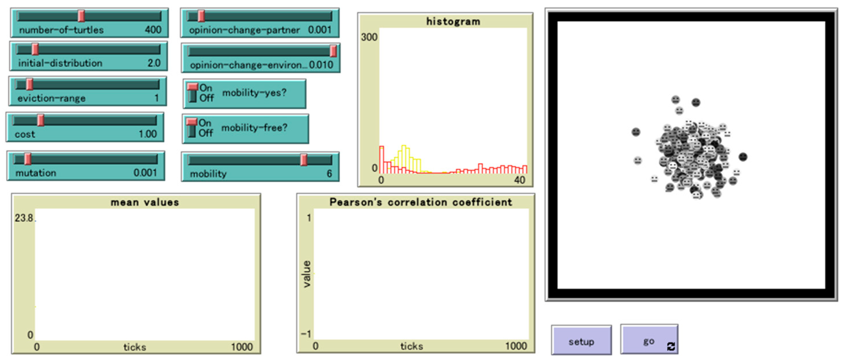
Figure 1 shows a screenshot of NetLogo. In this ABM, we set the number of agents as 400. The whiter the agent’s color, the more resources it has. Initially, all agents are gathered around the center of the world, given by the normal distribution (mean 0, standard deviation 2) as described above. However, agents change their locations through migrations.
Consider density cost as a variable that represents the various costs associated with high density (e.g., rent, commuting). The greater the number of agents, the fewer the agents with inadequate resources to withstand the high density. Moreover, these agents will likely be expelled from their current location. Equation (1) is provided as a condition for this expulsion. Agents for whom Equation (1) holds are forced to migrate to any of the eight surrounding patches. In the equation, the variable cost is the coefficient of density.
resource.i − cost × density.i < 0,
Hereafter, we set the value cost as 1.
Agents decide to migrate as follows. Agent i compares the density it experiences with that of the other arbitrarily selected patches it visits and considers migrating to the patch with a density closer to its own opinion. However, to visit, agents should have enough resources. Hence, we define the range of distances that agent i can visit, or range.i, by Equation (2). If the right-hand side is less than or equal to zero, the agent cannot visit other patches. Here, the variable mobility is the independent variable representing the possibility of visit and migration. The higher this value, the more agents can visit a wider range and select the patch for migration. The prevalence of both transportation technologies and ICTs should increase the variable mobility.
range.i = (resource.i − density.i) mobility.
Agent i visits one randomly selected patch within the range of its current patch. The density of the patch where agent i is present is density.i, and the density of the visited patch is visit.i. If Equation (3) below holds, agent i migrates to the visited patch. If Equation (3) does not hold, the migration is canceled, and the agent remains in the patch where they are present.
|opinion.i − density.i| > |opinion.i − visit.i|.
Next, agent i interacts with any agent who stays in the patch wherein agent i stays or the eight surrounding patches. Now, we name the selected other agent as agent j. The opinions of agents i and j change according to Equations (4) and (5). Variable δ represents a minute value, representing the change ratio of opinions through interaction with other agents’ opinions. The value is 0.01 or 0.001, as explained in the next section. If no other agents are present in the patch wherein agent i stays and the eight surrounding patches, agent i does not change its opinion.
opinion.i′ = (1 − δ) opinion.i + δ opinion.j.
opinion.j′ = (1 − δ) opinion.j + δ opinion.i.
After interaction with another agent, agent i changes its opinion according to Equation (6) (i.e., corresponding to the real density it experiences). Variable ε represents a minute quantity, representing the change ratio of opinions through interaction with the patch’s density. The value is 0.01, 0.001, or 0, as explained in the next section.
opinion.i′ = (1 − ε) opinion.i + ε density.i
After changing its opinion in response to the opinions of others and the real density it experiences as described by Equations (4)–(6), the agent’s opinion changes by ζ with a probability of 0.001, according to Equation (7). The value is randomly given in the range −1 < ζ < 1.
opinion.i′ = opinion.i + ζ …with probability 0.001
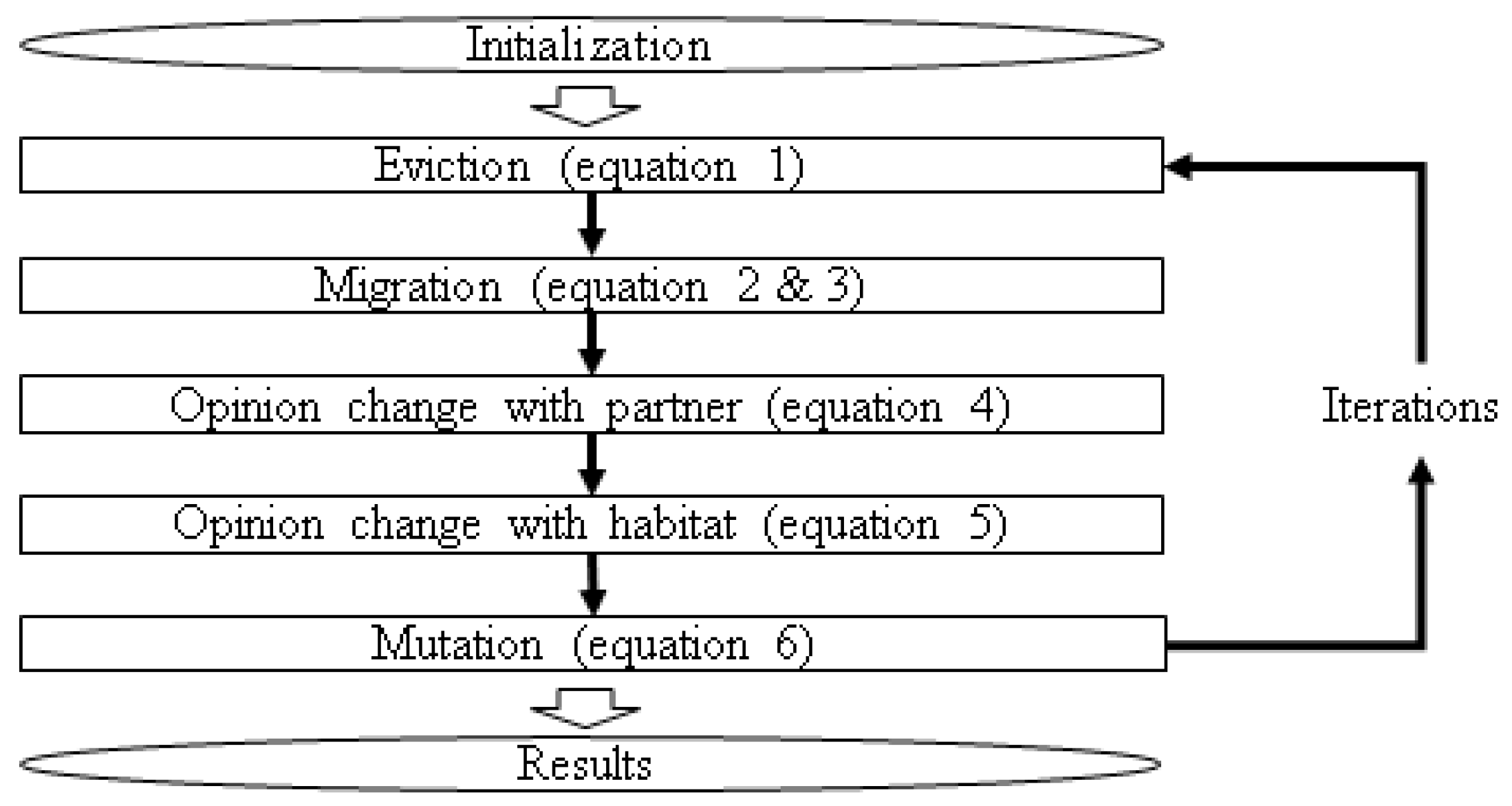
Figure 2 summarizes the above procedure. Agents are evicted, migrate, and change their opinion asynchronously following the orthodox assumption of NetLogo. One turn is completed when all agents follow the procedure. The model iterates the procedures sufficiently.
We changed variable δ for the change in opinion owing to interaction with other agents, variable ε for the change of opinion through the density of the patch, and, most importantly, the variable mobility. We particularly focus on the variable mobility. When transportation was poor and ICT did not exist, people could hardly visit any places and migrate; mobility was zero or low. In that case, people hardly migrate anywhere by choice, or migration may only be possible for the rich. The distance of migrations would have been limited. However, with the development of transportation and ICT, migration to a wider area will become possible for many people, corresponding to the increase in the value of mobility. Notably, the space assumed in the ABM is finite. In this ABM, the length of a piece of the patch is set to 31. If the value range in Equation (2) exceeds this length—exceeding 31 × √2 = 43.8 (the diagonal length of the patch)—virtually any location can be chosen. As mobility increases, these possibilities open up for many agents. This ABM primarily aims to clarify how interactions and disparities among agents change when the variable mobility changes from 0 to a larger value, including ∞, where all agents are free to move to any location.
To identify how the agents’ relationships change by varying the size of the independent variables, we focus on density.i and opinion.i. The higher these values are, the more the agents concentrate on an area of higher density and the more they desire such an environment. We also focus on diversity.i, which is the variance of resources of all agents in a total of nine patches in and around the patch where agent i stays. The larger this value is, the more agent i becomes co-located with other agents with diverse resources. This also suggests that the higher the diversity of the living environment, the less segregation there is of agents based on resources.
This study illustrates the disparity between agents in the resulting spatial distribution. Each agent has a different quantity of resources. How do density, opinion, and diversity differ depending on the agent’s resources? For all agents, we calculate the Pearson’s correlation coefficient between resources and each of the three dependent variables. We can then clarify how disparity varies depending on mobility differences by analyzing these variables.
4. Results
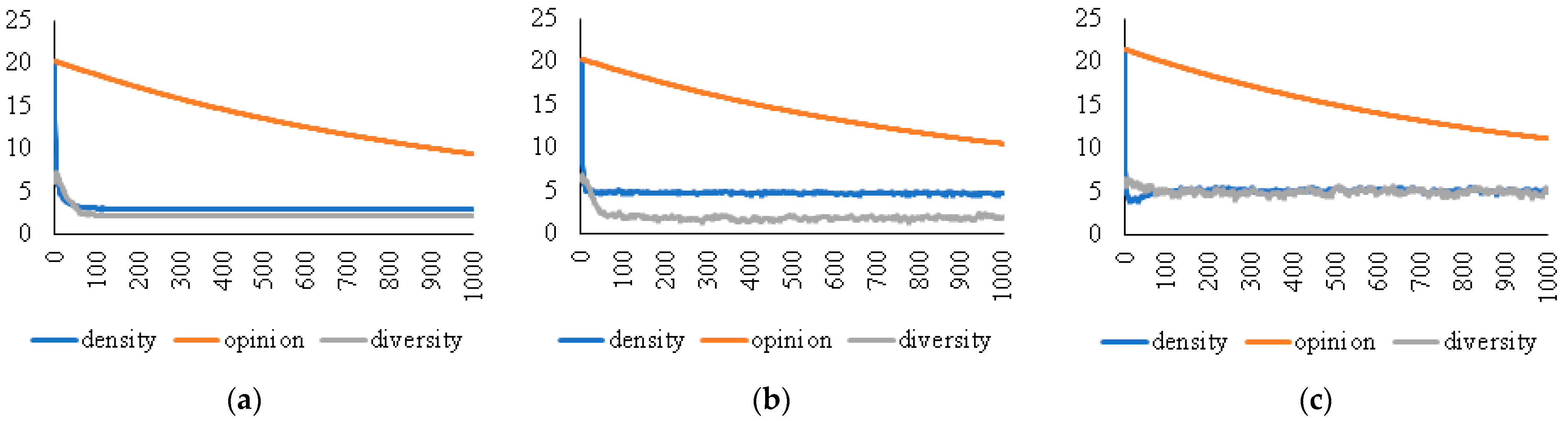
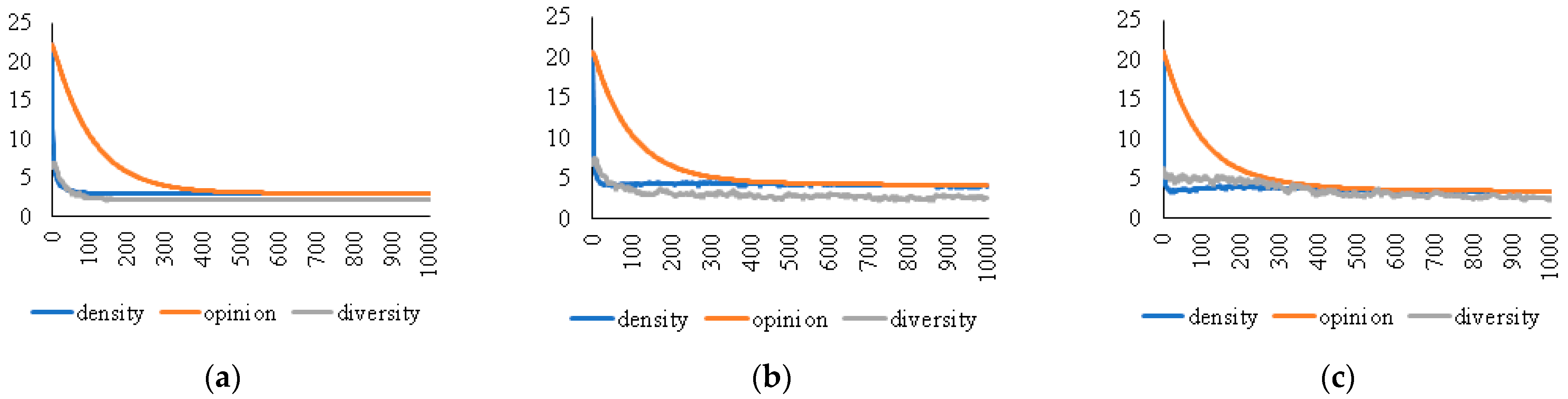
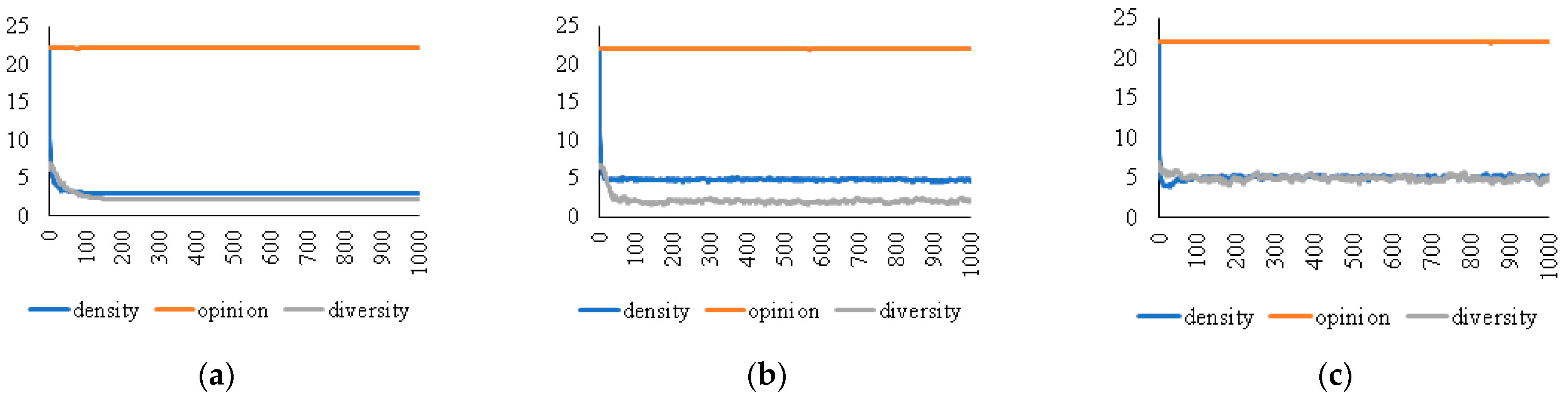
We show the results of one-shot simulations. We assume that agents change their opinions to a greater extent when they interact with other agents than when they experience a density of living environments. We set δ = 0.01 and ε = 0.001 (δ > ε). Figure 3 shows the change in the mean values of density, opinion, and diversity for three patterns: mobility = 0, 1, and ∞, along turns. The figures show the values of density and diversity saturate around turn 100, while opinion continues to decline. The possible range of opinion and density is 1/9 < opinion, density < 400/9. Actually, both values are within 5–20, due to the value of other variables, such as patch sizes, the number of agents, initial distribution of agents, and cost. Assuming that one turn corresponds to 1 week, 1000 weeks (or about 20 years) is a reasonable time frame for examining the results.
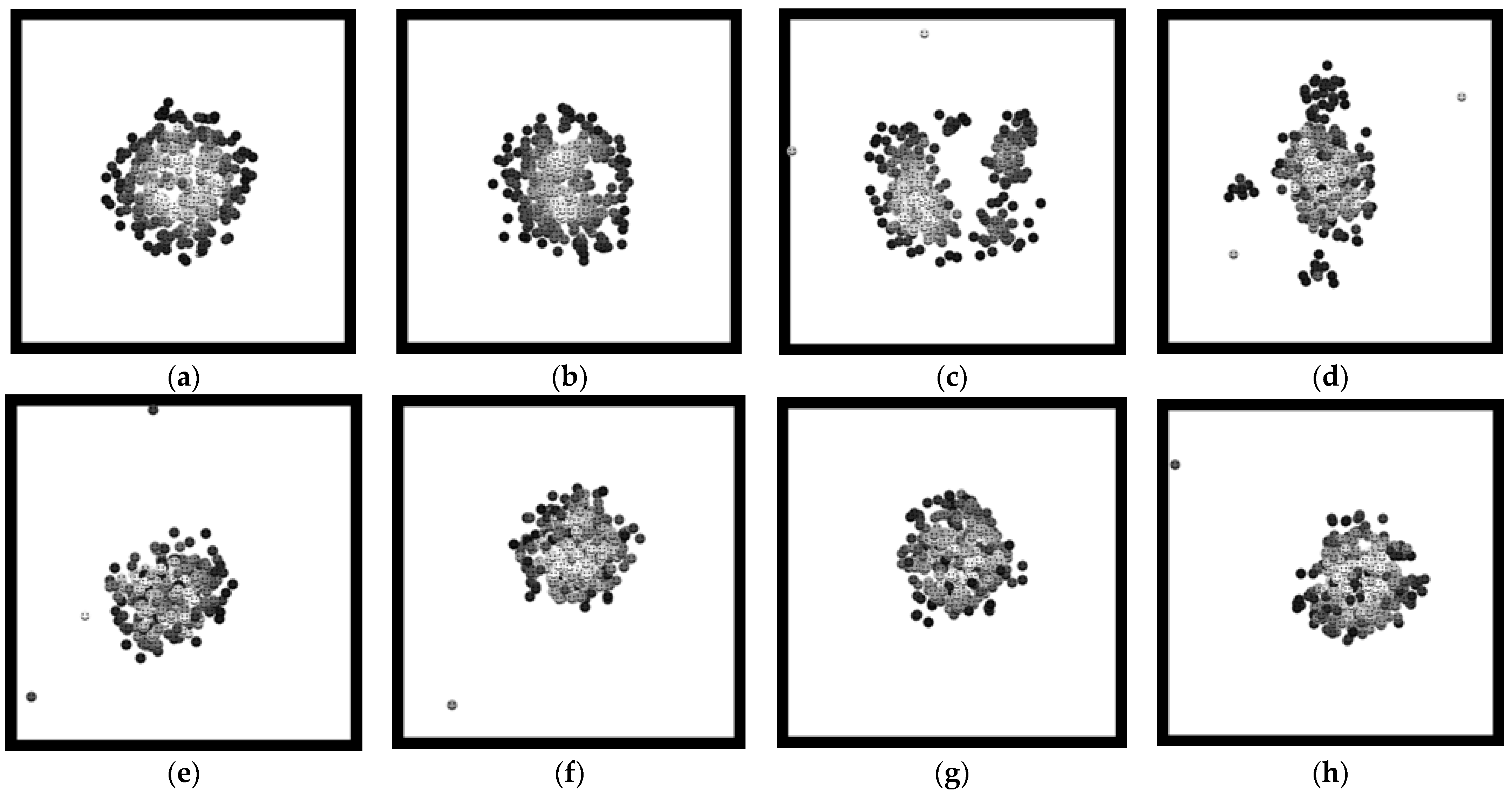
Figure 4 shows the distribution of agents after 1000 turns. We can see that the distribution of agents changes for different values of mobilities. When the value of mobility is small, agents scatter or segregate depending on resources (Figure 4a–d). When the value of mobility is high, many agents aggregate into a center irrespective of their resources; conversely, a few agents locate themselves far from the center (Figure 4e–h).
Table 1 shows the means and standard deviations of density, opinion, and diversity after 1000 turns. The table also presents the Pearson’s correlation coefficient between resource and each of the three variables. The mean value of each variable differs depending on the value of mobility. When the Pearson’s correlation coefficient is positive, the higher the resource, the higher the disparities. We focus on the correlation coefficients of resource and density. Correlation coefficients are positive and statistically significant at the 0.1% level in all conditions. However, the values differ depending on the value of mobility. The lowest value (i.e., the lowest disparity in terms of the correlation between resource and density) is for mobility = 4 (Table 1(e)).
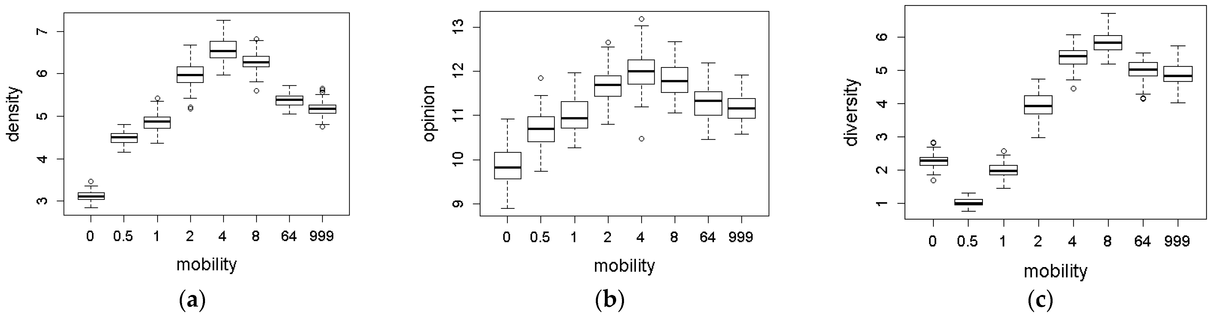
We gave different values of mobility corresponding to Figure 4 and Table 1, and we ran simulations for 100 trials for each mobility. Figure 5 shows box plots for the mean values of density, opinion, and diversity, respectively, with different values of mobility. The figures show that density increases as mobility increases, reaching its maximum value when the mobility is 4. However, as mobility further increases, density decreases. Moreover, the figures show that opinion shows similar results with density to the change in mobility, although they show higher values than density and with more variances. The figures show different patterns of diversity from those of density and opinion, with the change in mobility. The values show a minimum at the mobility of 0.5, followed by a maximum at the mobility of 8, and then a decrease as mobility further increases.
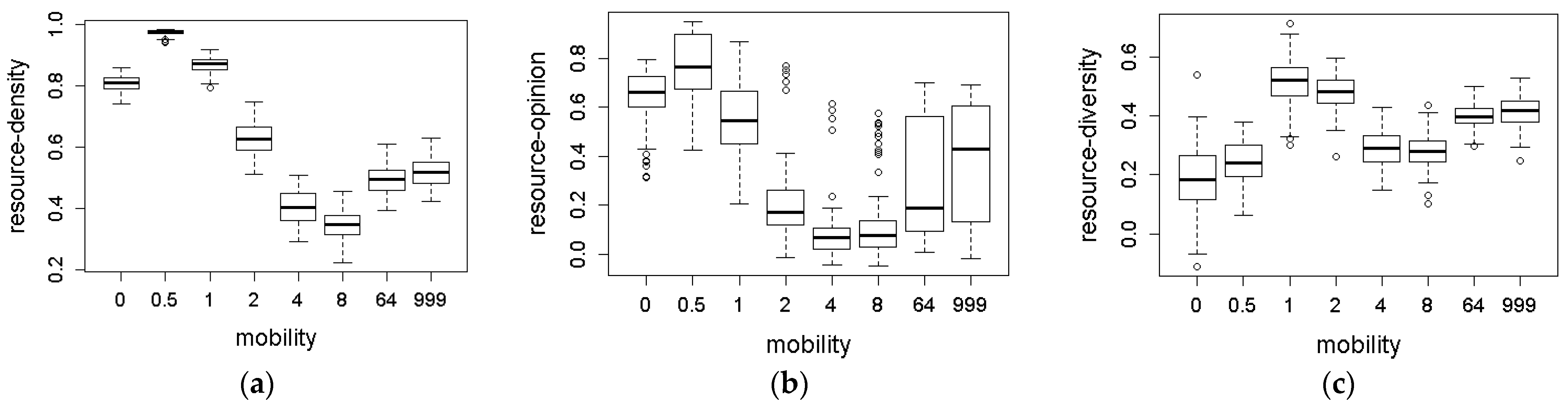
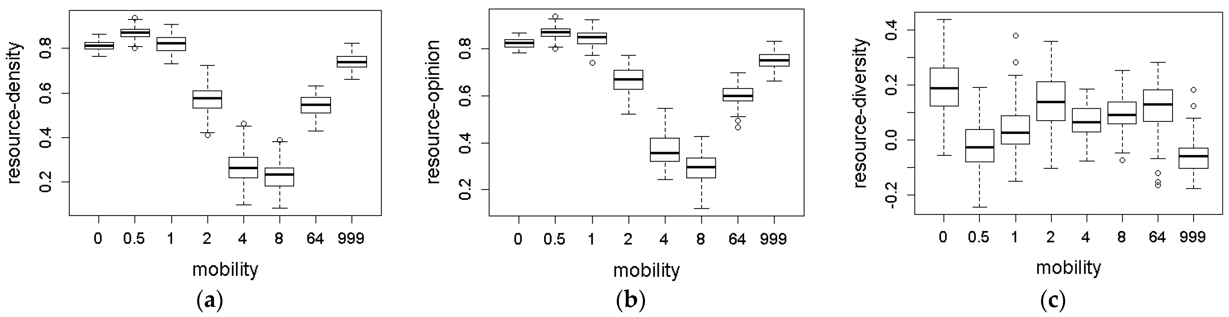
Figure 6 shows the box plots for the mean values of Pearson’s correlation coefficients between resource and density, opinion, and diversity, respectively, with different values of mobility. The correlation coefficients for resource and density show maximum and minimum values when the values of mobility are 0.5 and 8, respectively. The correlation coefficient between resource and opinion shows a similar pattern to that between resource and density, although with more variances. The correlation coefficient between resource and diversity shows a maximum value when mobility is 1.
We changed the values of δ and ε to δ = 0.001 and ε = 0.01. That is, we simulated the case wherein the change in opinion is not likely caused by interaction with other agents, but by adaptation to the density agents’ experience (δ < ε). Figure 7 shows the results of the one-shot simulations as in Figure 3. The value of opinions quickly converges to the value of densities.
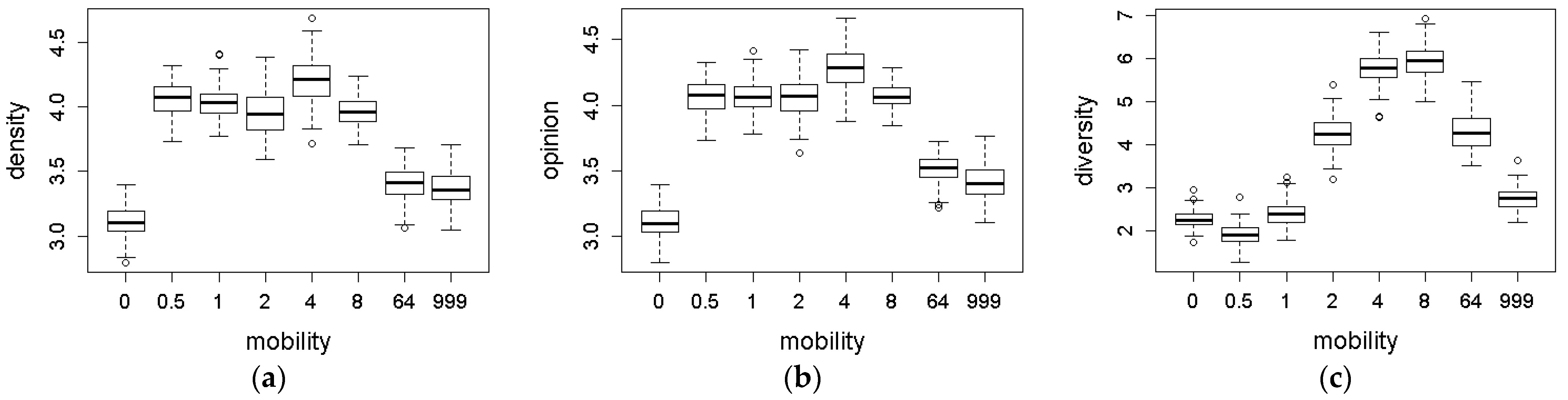
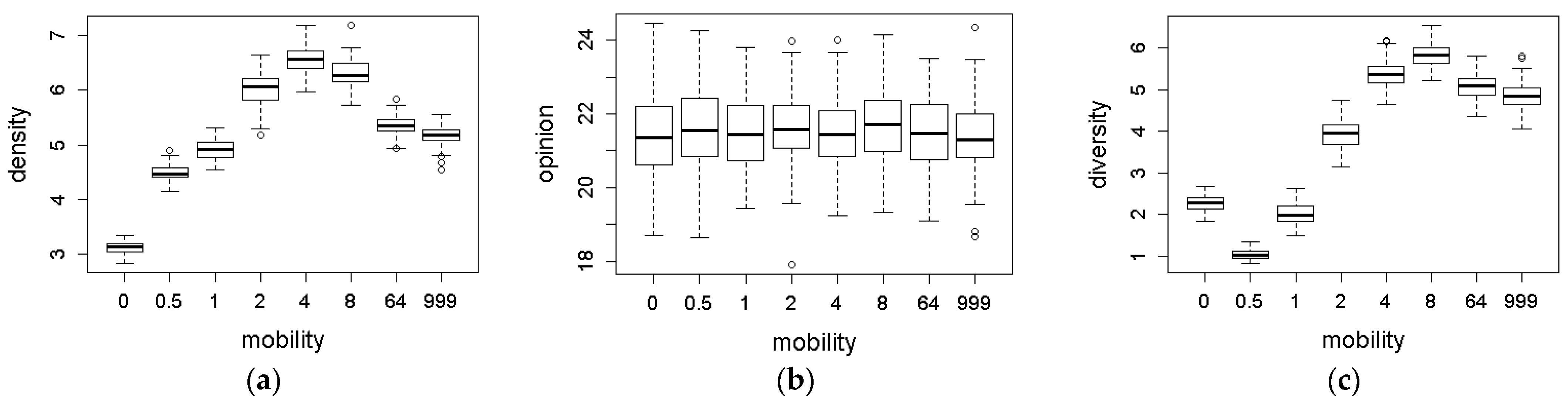
Figure 8 shows the box plots for the mean values of density, opinion, and diversity for each mobility. We also use the same procedure as in Figure 5 for 100 trials with each mobility. Figure 8 shows similar patterns to Figure 5. Compared with Figure 5, the mean values of density are smaller. Moreover, the mean values of opinions are smaller and similar to density. Notably, all three values—density, opinion, and diversity—are small when the value of mobility is high (i.e., mobility = 64 or ∞), compared with Figure 5.
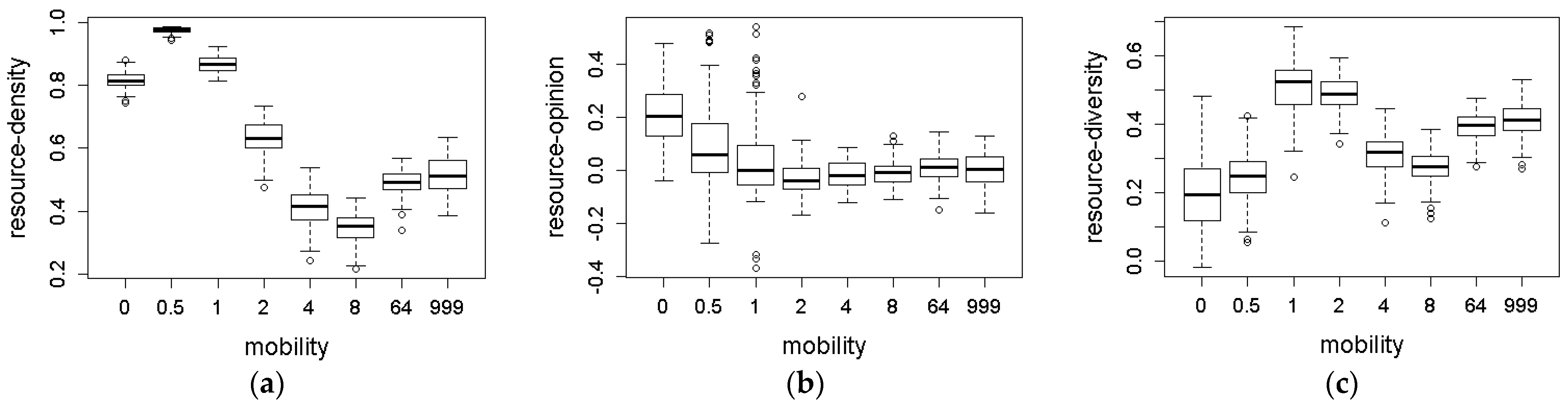
Figure 9 presents the results of the same simulation procedure as in Figure 6 for the Pearson’s correlation coefficients between resource and density, opinion, and diversity, respectively, for 100 trials with each mobility. The figures show patterns almost similar to Figure 6, except for cases of high mobility (64 or ∞). When mobility is high, agents face strong disparity in density and opinion, whereas less disparity in diversity.
We changed the values of δ and ε to δ = 0.01 and ε = 0. That is, we simulated the case wherein the change in opinion is caused only by interaction with other agents. Figure 10 shows the results of the one-shot simulations as in Figure 3. The value of opinion rarely changes as time passes.
Figure 11 shows the box plots for the mean values of density, opinion, and diversity for each mobility. We also use the same procedure as in Figure 5 for 100 trials with each mobility. Figure 11 shows similar patterns to Figure 5 in density and diversity. The mean values of opinions are not different for different values of mobility.
Figure 12 presents the results of the same simulation procedure as in Figure 6 for the Pearson’s correlation coefficients between resource and density, opinion, and diversity, respectively, for 100 trials with each mobility. The figures show patterns almost like those in Figure 6, except for the cases of opinion. With higher mobility, there is less disparity of opinion among agents.
5. Discussion
In this study, the analysis focused on the effects of mobility on interactions and disparities among agents. First, we considered that agents change their opinions more likely because of their interactions with others than their living environments, that is δ > ε. If mobility is 0, or if agents cannot migrate by their will, urban areas will adopt a structure wherein the places to live are determined by the disparity between rich and poor. Agents with many resources are in the center of high density, and those with few resources are forced into the periphery of low density. Urban area structures are determined by disparity relative to the resources they have. Agents who prefer higher densities tend to be those with more resources. As mobility increases slightly (0.5–2), agents can migrate more freely. However, this is only possible for those with abundant resources. Agents with many resources migrate to increasingly desirable high-density locations. Conversely, agents with fewer resources are pushed out from the patch of high density. As a result, urban concentration occurs and disparities relative to resources in densities and opinions widen. Moreover, we can find the segregation of agents based on the value of resources.
In primitive cities, the distribution of industrial structure, with industry in the center and agriculture on the periphery, has been explained by the classical von Thünen model [74]. In this model, the small mobility situation may reproduce that picture, albeit in a different model setting: as mobility increases slightly, only agents with more resources can migrate as they are mobile. Therefore, agents with few resources are pushed out, and more disparities in their areas arise, such as gentrification [21].
As mobility increases (4–8), agents with fewer resources can migrate to vacant urban centers. Conversely, agents with more resources who prefer lower densities suddenly emerge. Agents with fewer resources also reside in the gaps created by this migration of plentiful resources. As a result, agents with few resources will also reside in the gaps created by these migrant agents. Disparities between opinions and density based on the amounts of resources become smaller. The mean value of diversity is at the maximum, while disparities in diversity shrink in this mobility. Agents live with neighbors of different resources. As a result, agents enjoy high diversity.
Assume a situation where mobility increased, as in global cities, which attract people from all over the world. The high-density city has often been highlighted as a possible locus of disparity [27,28]. Conversely, this was also sometimes seen as a creative city where different people were involved, and innovation was expected [75,76,77]. This paper shows that in such high-mobility conditions, the disparity between people may be reduced in terms of density, opinion, and diversity among people with different resources. We may understand this situation as a just city [78,79,80] in which democracy, diversity, and equality are maintained, and urban space is created in a bottom-up manner through cooperation among people. In the studies [78,79,80], a just city was viewed as normative. By increasing mobility, we may attain a just city where different people come together and where disparities are reduced. How to interpret these results depends on one’s position, and this position differs depending on what criteria one uses to evaluate a city [81].
As mobility increases further (64–∞) and any agent can move to any location of its choosing, overall density will decrease as some agents will change and prefer low density. This is especially true for agents with few resources who are forced out of high-density areas. Moreover, we ran simulations when people changed their opinions based on their own experiences rather than through interactions with others (i.e., when δ < ε). The disparity tends to increase when mobility reaches very large values. The disparity increases owing to agents with few resources actively securing residences in low-density environments. The agents may be more satisfied in the sense of lower relative deprivation. However, this increases the disparity among agents. Following the classical opinion formation model, we also ran simulations in which agents change their opinions only through interactions with others (ε = 0) but we found scarce differences.
In extremely high mobility, people may move away from urban areas. They are more likely influenced by their living environments rather than by others. We have identified this as lifestyle migration [37,38,39]. Lifestyle migration, which now occurs in developed countries, has been enabled by the emergence of extremely mobile people, such as digital nomads [42,43]. This study suggests the new lifestyle seeking in rural areas may indicate a widening disparity among people. By having some people removed as if by their own will as digital nomads, wealthy people may monopolize the centers of global cities. Experimental research would be needed on how people move or how they determine their opinions for different densities.
This model has limitations. The model assumes that people will migrate flexibly, depending on their opinion regarding the density they seek. When the variable ‘mobility’ is high, people can migrate to distant and unfamiliar areas. In fact, even if there is a favorable density environment, people will not migrate so easily since their opinions change quickly. In this sense, the model depicts a hypothetical world in which people have lost their adherence to their residence, or the age of “Mobilities”, as Urry describes it [1]. If we want to make the model more relevant to today’s real world, we could, for example, add a variable ‘hesitation’ greater than 0 to the right-hand side of Equation (3). Assume that the greater the hesitation, people are less free to migrate. What this study models is a world where hesitation = 0. Future studies may look at the impact of hesitation. This model used only density as a factor for costs and migration. However, for example, global environmental destruction, disasters, and warfare may also be factors that worsen environments and encourage migration [46]. Moreover, agents may migrate not only according to the density they seek but also for diversity. Some people prefer to migrate to places where diverse groups of people gather as they believe that innovation will occur there [75,76,77]. Developing this model would be possible with such parameters in mind. The model assumes neighbor agents within nine patches as partners for opinion formation. However, if a strong connection is established through social networking across distant sites, the preferred density may be influenced not by the neighborhood or environment, but by distant familiar people, which may likely be people interacting through social networking services [82]. Moreover, the model assumes that if agents are neighbors, they would influence each other’s opinions. However, as shown in the opinion formation model, if opinions are quite distant from one another, they may not be influenced or may even rebel [61,62]. In those situations, variances of opinions would increase. In particular, the most important variable in this paper is resources. This may correspond to a person’s human or cultural capital. People may not interact with, be influenced by, or give their opinions to others whose resource values are too far apart from their own. They may more likely be influenced by those of similar resources and the same cultural capital [83]. This study assumed large cities that are already highly populated. It also assumed a democratic country where people can move of their will, although it depends on the amount of their resources. By changing the initial distribution of agents, density costs, and freedom of migration, we can extend the model to rural areas and countries/regions where freedom of movement is not guaranteed. Making such assumptions would be another possible development of this basic model, an issue that can be addressed in the future.
6. Conclusions
Segregation and gentrification are serious concerns in many megacities and global cities. Perhaps in reaction to this situation, lifestyle migration to the countryside is occurring among some people in developed countries. Lifestyle migration to the countryside, however, has not led to a reduction in disparities. It may simply make disparities less spatially visible. It is desirable to have a city in which different people can gather and interact with each other. We experimented with a hypothetical ABM to see what factors would be necessary for this to happen and found that the value of mobility is important.
This study shows that when mobility is too low or too high, disparities among people increase, and segregation, gentrification, or expulsion to depopulated areas will be experienced. At a moderate value of mobility, density, opinion, and diversity increase, and the disparity between people decreases. In the age of mobility, we should encourage people to move freely, but not too far away from their residential areas. It may be advisable to encourage people to find attached areas. People should also be encouraged to interact with each other not only to change their opinions but also to have affiliations with their neighbors. We may thus attain a just city where diverse people can live in high density with less disparity.
The present ABM is based on very simple assumptions. The ABM can be extended in various ways by adding new variables or changing the initial conditions. It may also be possible to consider specific urban planning by using actual GIS data, population data, etc. It is expected that future research will contribute to better urban development.
Supplementary Materials
The following supporting information can be downloaded at: https://www.mdpi.com/article/10.3390/computers12050094/s1, computers-12-00094-supplementary-Netlogo.
Funding
This study was supported by a JSPS KAKENHI grant number 21K12469.
Data Availability Statement
All data in this article were generated by an agent-based simulation program, which is available within Supplementary Materials.
Acknowledgments
The author would like to thank three anonymous reviewers for improving the manuscript.
Conflicts of Interest
The author declares no conflict of interest.
References
- Urry, J. Mobilities; Princeton University Press: Princeton, NJ, USA, 2007. [Google Scholar]
- Sheller, M. Advanced Introduction to Mobilities; Edward Elgar Publishing: Cheltenham, UK, 2020. [Google Scholar]
- Sik, E. Trust, Network Capital, and Informality? Cross-border entrepreneurship in the first two decades of post-communism. Rev. Sociol. 2012, 4, 53–72. [Google Scholar]
- Trupp, A. The development of ethnic minority souvenir business over time and space. Int. J. Asia Pac. Stud. 2015, 11, 145–167. [Google Scholar]
- Koltai, J.; Sik, E.; Simonovits, E. Network capital and migration potential. Int. J. Sociol. 2020, 50, 122–141. [Google Scholar] [CrossRef]
- Williams, A.M.; Hall, C.M. Tourism, migration, circulation and mobility. In Tourism and Migration: New Relationships between Production and Consumption; Williams, A.M., Hall, C.M., Eds.; Kluwer Academic Publishers: London, UK, 2002; pp. 1–60. [Google Scholar]
- Urry, J.; Larsen, J. The Tourist Gaze 3.0; Sage Publications: New York, NY, USA, 2011. [Google Scholar]
- Elliot, A.; Urry, J. Mobile Live; Routledge: London, UK, 2010. [Google Scholar]
- Larsen, J.; Urry, J.; Axhausen, K. Mobilities, Networks, Geographies; Routledge: London, UK, 2016. [Google Scholar]
- Dekker, R.; Engbersen, G. How social media transform migrant networks and facilitate migration. Glob. Netw. 2014, 14, 401–418. [Google Scholar] [CrossRef]
- Kim, M.J.; Lee, C.K.; Bonn, M. The effect of social capital and altruism on seniors’ revisit intention to social network sites for tourism-related purposes. Tour. Manag. 2016, 53, 96–107. [Google Scholar] [CrossRef]
- Kotyrlo, E. Impact of modern information and communication tools on international migration. Int. Migr. 2020, 58, 195–213. [Google Scholar] [CrossRef]
- Sheller, M. Mobility Justice: The Politics of Movement in an Age of Extremes; Verso: New York, NY, USA, 2018. [Google Scholar]
- Wu, F.; Zhang, F.; Webster, C. (Eds.) Rural Migrants in Urban China: Enclaves and Transient Urbanism; Routledge: New York, NY, USA, 2014. [Google Scholar]
- Hu, R. Competitiveness, migration, and mobility in the global city: Insights from Sydney, Australia. Economies 2015, 3, 37–54. [Google Scholar] [CrossRef]
- Wajdi, N.; Mulder, C.H.; Adioetomo, S.M. Inter-regional migration in Indonesia: A micro approach. J. Popul. Res. 2017, 34, 253–277. [Google Scholar] [CrossRef]
- Haas, T.; Westlund, H. (Eds.) Emergent Transformation of Cities and Regions in the Innovative Global Economy; Routledge: London, UK, 2018. [Google Scholar]
- Champion, T.; Cooke, T.; Shuttleworth, I. (Eds.) Internal Migration in the Developed World: Are We Becoming Less Mobile? Routledge: New York, NY, USA, 2018. [Google Scholar]
- Alghais, N.; Pullar, D.; Charles-Edward, E. Accounting for peoples’ preferences in establishing new cities: A spatial model of population migration in Kuwait. PLoS ONE 2018, 13, e0209065. [Google Scholar] [CrossRef]
- Zhu, J.; Zhu, M.; Xiao, Y. Urbanization for rural development: Spatial paradigm shifts toward inclusive urban-rural integrated development in China. J. Rural Stud. 2019, 71, 94–103. [Google Scholar] [CrossRef]
- Smith, N. The New Urban Frontier: Gentrification and the Revanchist City; Routledge: London, UK, 1996. [Google Scholar]
- Lees, L.; Slater, T.; Wyly, E. Gentrification; Routledge: London, UK, 2008. [Google Scholar]
- Lees, L.; Shin, H.B.; Lopez-Morales, E. Global Gentrification: Uneven Development and Displacement; Policy Press: Bristol, UK, 2015. [Google Scholar]
- Lees, L.; Shin, H.B.; Lopez-Morales, E. Planetary Gentrification; Routledge: London, UK, 2016. [Google Scholar]
- Colomb, C.; Novy, J. Protest and Resistance in the Tourist City; Routledge: London, UK, 2016. [Google Scholar]
- Gravari-Barbas, M.; Guinand, S. Tourism and Gentrification in Contemporary Metropolises: International Perspectives; Routledge: London, UK, 2017. [Google Scholar]
- Sassen, S. The Global City: NewYork, London, Tokyo; Princeton University Press: Princeton, NJ, USA, 2001. [Google Scholar]
- Sassen, S. Cities in a World Economy, 5th ed.; Sage Publisher: NewYork, NY, USA, 2019. [Google Scholar]
- Gans, H.J. The Urban Villagers: Group and Class in the Life of Italian-Americans; Simon and Schuster: New York, NY, USA, 1982. [Google Scholar]
- Davis, M. City of Quartz: Excavating the Future in Los Angeles; Verso: New York, NY, USA, 1990. [Google Scholar]
- Cheng, Y.; Rosenberg, M.; Winterton, R.; Blackberry, I.; Gao, S. Mobilities of older Chinese rural-urban migrants: A case study in Beijing. Int. J. Enviorn. Res. Public Health 2019, 16, 488. [Google Scholar] [CrossRef]
- Spray, J.; Witten, K.; Wiles, J.; Anderson, A.; Paul, D.; Wade, J.; Ameratunga, S. Inequitable mobilities: Intersections of diversity with urban infrastructure influence mobility, health and wellbeing. Cities Health 2022, 6, 711–725. [Google Scholar] [CrossRef]
- Chen, Y.; Xi, H.; Jiao, J. What are the relationships between public transit and gentrification progress? An empirical study in the New York: Northern New Jersey-Long Island areas. Land 2023, 12, 358. [Google Scholar] [CrossRef]
- Florida, R. The New Urban Crisis: How Our Cities Are Increasing Inequality, Keeping Segregation, and Failing the Middle Class and What We Can Do about It; Basic Books: New York, NY, USA, 2017. [Google Scholar]
- Shi, J.; Duan, K.; Xu, Q.; Li, J. Effect analysis of the driving factors of super- gentrification using structural equation modeling. PLoS ONE 2021, 16, e0248265. [Google Scholar] [CrossRef]
- Barbarossa, L. The post pandemic city: Challenges and opportunities for a non-motorized urban environment. An overview of Italian cases. Sustainability 2020, 12, 7172. [Google Scholar] [CrossRef]
- Benson, M.; O’Reilly, K. (Eds.) Lifestyle Migration: Expectations, Aspirations and Experiences; Routledge: London, UK, 2009. [Google Scholar]
- Benson, M.; O’Reilly, K. (Eds.) Understanding Lifestyle Migration: Theoretical Approaches to Migration and the Quest for a Better Way of Life; Palgrave Macmillan: London, UK, 2014. [Google Scholar]
- Klien, S. Urban Migrants in Rural Japan: Between Agency and Anomie in a Post-Growth Society; Suny Press: New York, NY, USA, 2020. [Google Scholar]
- Bauman, Z. Liquid Modernity; Polity: Cambridge, UK, 2000. [Google Scholar]
- Bauman, Z. Community: Seeking Safety in an Insecure World; Polity: Cambridge, UK, 2001. [Google Scholar]
- Green, P. Disruptions of self, place and mobility: Digital nomads in Chiang Mai, Thailand. Mobilities 2020, 15, 431–445. [Google Scholar] [CrossRef]
- Hannonen, O. In search of a digital nomad: Defining the phenomenon. Inf. Tech. Tour. 2020, 22, 335–353. [Google Scholar] [CrossRef]
- Espíndola, A.L.; Silveira, J.L.; Penna, T.J.P. A Harris-Todaro agent-based model to rural-urban migration. Braz. J. Phys. 2006, 36, 603–609. [Google Scholar] [CrossRef]
- Silveira, J.J.; Espíndola, A.L.; Penna, T.J.P. An agent-based model to rural-urban migration analysis. Phys. A Stat. Mech. Its Appl. 2006, 364, 445–456. [Google Scholar] [CrossRef]
- Klabunde, A.; Willekens, F. Decision-making in agent-based models of migration: State of the art and challenges. Eur. J. Popul. 2016, 32, 73–97. [Google Scholar] [CrossRef]
- Nguyen, H.K.; Chiong, R.; Chica, M.; Middleton, R.H. Understanding the dynamics of inter-provincial migration in the Mekong Delta, Vietnam: An agent-based modeling study. Simulation 2021, 97, 267–285. [Google Scholar] [CrossRef]
- Torrens, P.M.; Nara, A. Modeling gentrification dynamics: A hybrid approach. Comput. Environ. Urban Syst. 2007, 31, 337–361. [Google Scholar] [CrossRef]
- Termos, A.; Picascia, S.; Yorke-Smith, N. Agent-based simulation of west Asian urban dynamics: Impact of refugees. J. Artif. Soc. Soc. Simul. 2021, 24, 2. [Google Scholar] [CrossRef]
- Schelling, T.C. Dynamic models of segregation. J. Math. Sociol. 1971, 1, 143–186. [Google Scholar] [CrossRef]
- Malik, A.; Abdalla, R. Agent-based modelling for urban sprawl in the region of Waterloo, Ontario, Canada. Model. Earth Syst. Environ. 2017, 3, 7. [Google Scholar] [CrossRef]
- Sahasranaman, A.; Jensen, H.J. Cooperative dynamics of neighborhood economic status in cities. PLoS ONE 2017, 12, e0183468. [Google Scholar] [CrossRef]
- Fu, Z.; Hao, L. Agent-based modeling of China’s rural-urban migration and social network structure. Phys. A Stat. Mech. Its Appl. 2018, 490, 1061–1075. [Google Scholar] [CrossRef]
- Chen, Y.; Irwin, E.; Jayaprakash, C.; Park, K.J. An agent based model of a thinly traded land market in an urbanizing region. J. Artif. Soc. Soc. Simul. 2021, 24, 1. [Google Scholar] [CrossRef]
- Horiuchi, S. Bridging of different sites by bohemians and tourists; analysis by agent based simulation. J. Comput. Soc. Sci. 2021, 4, 567–584. [Google Scholar] [CrossRef]
- Nagai, H.; Kurahashi, S. Agent-based modeling of the formation and prevention of residential diffusion on urban edges. Sustainability 2021, 13, 12500. [Google Scholar] [CrossRef]
- Kajiwara, K.; Ma, J.; Seto, T.; Sekimoto, T.; Ogawa, Y.; Omata, H. 2022. Development of current estimated household data and agent-based simulation of the future population distribution of households in Japan. Comput. Environ. Urban Syst. 2022, 98, 101873. [Google Scholar] [CrossRef]
- Deffuant, G.; Neau, D.; Amblard, F.; Weisbuch, G. Mixing beliefs among interacting agents. Adv. Complex Syst. 2001, 3, 87–98. [Google Scholar] [CrossRef]
- Deffuant, G.; Amblard, F.; Weisbuch, G.; Faure, T. How can extremism prevail? A study on the relative agreement interaction model. J. Artif. Soc. Soc. Simul. 2002, 5, 4. [Google Scholar]
- Deffuant, G.; Huet, S.; Amblard, F. An individual-based model of innovation diffusion mixing social value and individual benefit. Am. J. Sociol. 2005, 110, 1041–1069. [Google Scholar] [CrossRef]
- Weisbuch, G.; Deffuant, G.; Amblard, F.; Nadal, J. Meet, discuss, and segregate! Complexity 2002, 7, 55–63. [Google Scholar] [CrossRef]
- Weisbuch, G.; Deffuant, G.; Amblard, F.; Nadal, J. Persuasion dynamics. Phys. A Stat. Mech. Its Appl. 2005, 353, 555–575. [Google Scholar] [CrossRef]
- Xia, H.; Wang, H.; Xuan, Z. Opinion dynamics: A multidisciplinary review and perspective on future research. Int. J. Knowl. Syst. Sci. 2011, 2, 72–91. [Google Scholar] [CrossRef]
- Li, J.; Xiao, R. Agent-based modelling approach for multidimensional opinion polarization in collective behaviour. J. Artif. Soc. Soc. Simul. 2017, 20, 4. [Google Scholar] [CrossRef]
- Muller, S.T.; Tan, Y.S. Cognitive perspectives on opinion dynamics: The role of knowledge in consensus formation, opinion divergence, and group polarization. J. Comput. Soc. Sci. 2018, 1, 15–48. [Google Scholar] [CrossRef]
- Chen, T.; Li, Q.; Yang, J.; Cong, G.; Li, G. Modeling of the public opinion polarization process with the considerations of individual heterogeneity and dynamic conformity. Mathematics 2019, 7, 917. [Google Scholar] [CrossRef]
- Gracia-Lazaro, C.; Floria, L.M.; Moreno, Y. Selective advantage of tolerant cultural traits in the Axelrod-Schelling model. Phys. Rev. E 2011, 83, 56103. [Google Scholar] [CrossRef] [PubMed]
- Cai, N.; Ma, H.Y.; Khan, M.J. Agent-based model for rural-urban migration: A dynamic consideration. Phys. A Stat. Mech. Its Appl. 2015, 436, 806–813. [Google Scholar] [CrossRef]
- Alraddadi, E.E.; Allen, S.M.; Colombo, G.B.; Whitaker, R.M. The role of homophily in opinion formation among mobile agents. J. Inf. Telecommun. 2020, 4, 504–523. [Google Scholar] [CrossRef]
- Wilensky, U. NetLogo. Center for Connected Learning and Computer-Based Modeling. Northwestern University: Evanston, IL, USA, 1999. Available online: http://ccl.northwestern.edu/netlogo (accessed on 3 September 2021).
- Diappi, L.; Bolchi, P. Smith’s rent gap theory and local real estate dynamics: A multi-agent model. Comput. Environ. Urban Syst. 2008, 32, 6–18. [Google Scholar] [CrossRef]
- Perez, L.; Dragicevic, S.; Gaudreau, J. A geospatial agent-based model of the spatial urban dynamics of immigrant population: A study of the island of Montreal, Canada. PLoS ONE 2019, 14, e0219188. [Google Scholar] [CrossRef]
- Wahyudi, A.; Liu, Y.; Corcoran, J. Generating different urban land configurations based on heterogeneous decisions of private land developers: An agent-based approach in a developing country context. ISPRS Int. J. Geo-Inf. 2019, 8, 229. [Google Scholar] [CrossRef]
- Han, H.; Yuan, Z.; Zou, K. Agricultural location and crop choices in China: A revisitation on von Thünen model. Land 2022, 11, 1885. [Google Scholar] [CrossRef]
- Jacobs, J. The Death and Life of Great American Cities; Random House Publishing: New York, NY, USA, 1961. [Google Scholar]
- Zukin, S. Loft Living: Culture and Capital in Urban Change; Rutgers University Press: New Brunswick, NJ, USA, 1989. [Google Scholar]
- Florida, R. The Rise of the Creative Class Revisited; Basic Books: New York, NY, USA, 2012. [Google Scholar]
- Harvey, D. Social Justice and the City; University of Georgia Press: Athens, GA, USA, 2010. [Google Scholar]
- Fainstein, S.S. The Just City; Cornell University Press: New York, NY, USA, 2010. [Google Scholar]
- Soja, E.W. Seeking Spatial Justice; University of Minnesota Press: Minneapolis, MN, USA, 2010. [Google Scholar]
- Hatuka, T.; Rosen-Zvi, I.; Birnhack, M.; Toch, E.; Zur, H. The political premises of contemporary urban concepts: The global city, the sustainable city, the resilient city, the creative city, and the smart city. Plan. Theory Pract. 2018, 19, 160–179. [Google Scholar] [CrossRef]
- Okada, I.; Okano, N.; Ishii, A. Spatial opinion dynamics incorporating both positive and negative influence in small-world networks. Front. Phys. 2022, 10, 953184. [Google Scholar] [CrossRef]
- Bourdieu, P. La Distinction: Critique Sociale du Jugement; Éditions de Minuit: Paris, France, 1979. [Google Scholar]
Figure 1.
Screenshot of the initial condition by NetLogo. In histogram red bars represent opinions, yellow bars represent diversity of agents.
Figure 1.
Screenshot of the initial condition by NetLogo. In histogram red bars represent opinions, yellow bars represent diversity of agents.

Figure 2.
The procedure of the ABM.

Figure 3.
Trends in the mean values of density, opinion, and diversity. The values of δ = 0.01 and ε = 0.001. The value of mobility = (a) 0, (b) 1, and (c) ∞.
Figure 3.
Trends in the mean values of density, opinion, and diversity. The values of δ = 0.01 and ε = 0.001. The value of mobility = (a) 0, (b) 1, and (c) ∞.

Figure 4.
Distribution of agents after 1000 turns. The values of δ = 0.01 and ε = 0.001. The value of mobility = (a) 0, (b) 0.5, (c) 1, (d) 2, (e) 4, (f) 8, (g) 64, and (h) ∞.
Figure 4.
Distribution of agents after 1000 turns. The values of δ = 0.01 and ε = 0.001. The value of mobility = (a) 0, (b) 0.5, (c) 1, (d) 2, (e) 4, (f) 8, (g) 64, and (h) ∞.

Figure 5.
Box plot for the mean values of (a) density, (b) opinion, and (c) diversity for mobility (x-axes) after 1000 turns with 100 trials; 999 in the x-axis represents ∞ and ◦ represents outliers. The values of δ = 0.01 and ε = 0.001.
Figure 5.
Box plot for the mean values of (a) density, (b) opinion, and (c) diversity for mobility (x-axes) after 1000 turns with 100 trials; 999 in the x-axis represents ∞ and ◦ represents outliers. The values of δ = 0.01 and ε = 0.001.

Figure 6.
Box plots for Pearson’s correlation coefficients for (a) resource–density, (b) resource–opinion, and (c) resource–diversity at each mobility after 1000 turns with 100 trials; 999 in the x-axis represents ∞ and ◦ represents outliers. The values of δ = 0.01 and ε = 0.001.
Figure 6.
Box plots for Pearson’s correlation coefficients for (a) resource–density, (b) resource–opinion, and (c) resource–diversity at each mobility after 1000 turns with 100 trials; 999 in the x-axis represents ∞ and ◦ represents outliers. The values of δ = 0.01 and ε = 0.001.

Figure 7.
Trends in the mean values of density, opinion, and diversity. The values of δ = 0.001 and ε = 0.01. The value of mobility = (a) 0, (b) 1, and (c) ∞.
Figure 7.
Trends in the mean values of density, opinion, and diversity. The values of δ = 0.001 and ε = 0.01. The value of mobility = (a) 0, (b) 1, and (c) ∞.

Figure 8.
Box plot for the mean values of (a) density, (b) opinion, and (c) diversity at each mobility after 1000 turns with 100 trials; 999 in the x-axis represents ∞ and ◦ represents outliers. The values of δ = 0.001 and ε = 0.01.
Figure 8.
Box plot for the mean values of (a) density, (b) opinion, and (c) diversity at each mobility after 1000 turns with 100 trials; 999 in the x-axis represents ∞ and ◦ represents outliers. The values of δ = 0.001 and ε = 0.01.

Figure 9.
Box plots of Pearson’s correlation coefficients for (a) resource–density, (b) resource–opinion, and (c) resource–diversity at each mobility after 1000 turns with 100 trials; 999 in the x-axis represents ∞ and ◦ represents outliers. The values of δ = 0.001 and ε = 0.01.
Figure 9.
Box plots of Pearson’s correlation coefficients for (a) resource–density, (b) resource–opinion, and (c) resource–diversity at each mobility after 1000 turns with 100 trials; 999 in the x-axis represents ∞ and ◦ represents outliers. The values of δ = 0.001 and ε = 0.01.

Figure 10.
Trends in the mean values of density, opinion, and diversity. The values of δ = 0.01 and ε = 0. The value of mobility = (a) 0, (b) 1, and (c) ∞.
Figure 10.
Trends in the mean values of density, opinion, and diversity. The values of δ = 0.01 and ε = 0. The value of mobility = (a) 0, (b) 1, and (c) ∞.

Figure 11.
Box plot for the mean values of (a) density, (b) opinion, and (c) diversity at each mobility after 1000 turns with 100 trials; 999 in the x-axis represents ∞ and ◦ represents outliers. The values of δ = 0.01 and ε = 0.
Figure 11.
Box plot for the mean values of (a) density, (b) opinion, and (c) diversity at each mobility after 1000 turns with 100 trials; 999 in the x-axis represents ∞ and ◦ represents outliers. The values of δ = 0.01 and ε = 0.

Figure 12.
Box plots for Pearson’s correlation coefficients (a) resource–density, (b) resource–opinion, and (c) resource–diversity at each mobility after 1000 turns with 100 trials for each mobility; 999 in the x-axis represents ∞ and ◦ represents outliers. The values of δ = 0.01 and ε = 0.
Figure 12.
Box plots for Pearson’s correlation coefficients (a) resource–density, (b) resource–opinion, and (c) resource–diversity at each mobility after 1000 turns with 100 trials for each mobility; 999 in the x-axis represents ∞ and ◦ represents outliers. The values of δ = 0.01 and ε = 0.


Table 1.
Mean value and standard deviation of each variable and Pearson’s correlation coefficient with resource. * p < 0.001; the values of δ = 0.01 and ε = 0.001; mobility = (a) 0, (b) 0.5, (c) 1, (d) 2, (e) 4, (f) 8, (g) 64, and (h) ∞.
Table 1.
Mean value and standard deviation of each variable and Pearson’s correlation coefficient with resource. * p < 0.001; the values of δ = 0.01 and ε = 0.001; mobility = (a) 0, (b) 0.5, (c) 1, (d) 2, (e) 4, (f) 8, (g) 64, and (h) ∞.
| Density | Opinion | Diversity | ||
|---|---|---|---|---|
| (a) | Mean (SD) Correlation with resource | 3.04 (1.26) 0.792 * | 9.40 (0.40) 0.705 * | 2.11 (1.26) 0.287 * |
| (b) | Mean (SD) Correlation with resource | 4.40 (2.50) 0.979 * | 11.48 (0.83) 0.882 * | 1.06 (0.84) 0.228 * |
| (c) | Mean (SD) Correlation with resource | 4.76 (2.78) 0.872 * | 10.48 (1.00) 0.489 * | 1.92 (1.40) 0.514 * |
| (d) | Mean (SD) Correlation with resource | 5.49 (2.77) 0.676 * | 10.76 (0.89) 0.316 * | 3.71 (1.88) 0.583 * |
| (e) | Mean (SD) Correlation with resource | 6.90 (3.16) 0.326 * | 12.13 (1.06) 0.092 | 5.87 (2.18) 0.292 * |
| (f) | Mean (SD) Correlation with resource | 5.94 (2.38) 0.458 * | 11.25 (0.57) 0.093 | 5.57 (1.98) 0.285 * |
| (g) | Mean (SD) Correlation with resource | 5.33 (2.10) 0.792 * | 11.81 (0.12) 0.705 * | 5.09 (2.71) 0.287 * |
| (h) | Mean (SD) Correlation with resource | 4.90 (1.93) 0.518 * | 11.12 (0.57) 0.173 * | 4.90 (2.76) 0.341 * |
Disclaimer/Publisher’s Note: The statements, opinions and data contained in all publications are solely those of the individual author(s) and contributor(s) and not of MDPI and/or the editor(s). MDPI and/or the editor(s) disclaim responsibility for any injury to people or property resulting from any ideas, methods, instructions or products referred to in the content. |
© 2023 by the author. Licensee MDPI, Basel, Switzerland. This article is an open access article distributed under the terms and conditions of the Creative Commons Attribution (CC BY) license (https://creativecommons.org/licenses/by/4.0/).
Share and Cite
MDPI and ACS Style
Horiuchi, S. Disparity of Density in the Age of Mobility: Analysis by Opinion Formation Model. Computers 2023, 12, 94. https://doi.org/10.3390/computers12050094
AMA Style
Horiuchi S. Disparity of Density in the Age of Mobility: Analysis by Opinion Formation Model. Computers. 2023; 12(5):94. https://doi.org/10.3390/computers12050094
Chicago/Turabian StyleHoriuchi, Shiro. 2023. "Disparity of Density in the Age of Mobility: Analysis by Opinion Formation Model" Computers 12, no. 5: 94. https://doi.org/10.3390/computers12050094
Note that from the first issue of 2016, this journal uses article numbers instead of page numbers. See further details here.