Design and Simulation-Based Optimization of an Intelligent Autonomous Cruise Control System

Abstract

Significant progress has recently been made in transportation automation to alleviate human faults in traffic flow. Recent breakthroughs in artificial intelligence have provided justification for replacing human drivers with digital control systems. This paper proposes the design of a self-adaptive real-time cruise control system to enable path-following control of autonomous ground vehicles so that a self-driving car can drive along a road while following a lead vehicle. To achieve the cooperative objectives, we use a multi-agent deep reinforcement learning (MADRL) technique, including one agent to control the acceleration and another agent to operate the steering control. Since the steering of an autonomous automobile could be adjusted by a stepper motor, a well-known DQN agent is considered to provide the discrete angle values for the closed-loop lateral control. We performed a simulation-based analysis to evaluate the efficacy of the proposed MADRL path following control for autonomous vehicles (AVs). Moreover, we carried out a thorough comparison with two state-of-the-art controllers to examine the accuracy and effectiveness of our proposed control system.

1. Introduction

With the rapid technological advances, autonomous vehicles have received extensive attention in the past decade [1,2]. Increasing safety by computers has led to considerable benefits, including omitting human errors in critical circumstances, improving occupants’ comfort, reducing traffic problems, and reducing environmental impacts, which are among the main impetuses for the automation of driving. Any autonomous driving system consists of several perception level tasks, which must be considered for the design of such a system. Autonomous driving tasks are normally divided into three categories, namely navigation, guidance, and stabilization [3]. Although autonomous vehicles have the potential to revolutionize the transportation industry, there are significant risks associated with their use that must be taken into account, such as cybersecurity concerns, technical failures, and ethical implications. One of the major challenges in self-driving cars is the path following control in which the vehicle keeps the cruise velocity and a safe distance while following another vehicle simultaneously.

Different practical control methodologies have been studied to deliver the capability to keep the cruise velocity and safe distance, such as active steering [3], differential braking [4], integrated chassis control [5] and torque vectoring [6]. In particular, the driver-assist system, which has been extended in [7], enables better lane-keeping and tracking control. In [8], the authors presented a smooth route control for autonomous transport satisfying both the initial and final circumstances, where the restriction conditions are implemented as a parameterized 6th-order polynomial model [9]. In such a study, the tracking control module along with the model predictive control technique were used. In [10], a developed Kalman filter and linear time-varying model predictive control scheme are applied to predict the future trajectory of an autonomous vehicle (AV), determine the optimal path, and optimize control [9]. A common denominating challenge for the use of machine learning in designing autonomous control applications is the dependency of the decision making no training data, where experiencing learning data that is completely different from training data may lead to inconsistent decisions.

Designing control systems to regulate both throttle and brake is the key part of adaptive cruise control since it ensures the vehicle will keep the speed response of the antecedent vehicle, and consequently retaining a safe inter-vehicle distance under the limitations of driving [11]. In [12], an adaptive cruise control structure considering a variety of funnel controllers are introduced. In [13], the authors presented a least-violating control in the application of cruise control to regulate the system with the properties of safety, uniform reachability, and uniform attractivity. In [14], a varying prediction zone nonlinear model predictive control (NMPC) using a continuation/generalized minimal residual (C/GMRES) optimizer with a dead zone penalty function to guarantee the smoothness and meet the inequalities is designed in the path-following control application. A sliding mode control for speed control in AVs has been applied in [15]. Robust H-infinity control methods are investigated in [16]. A super-twisting sliding mode is presented in [17] based on Lyapunov stability proofed by the backstepping method in the application field of AVs path-following control. These methods demonstrated acceptable outcomes based on analytic control; they require not only complex design but also, are unable to consider unknown uncertainties due to the intense dynamic structure of automobiles. Thus, focusing on the complete mathematical model is impractical. To address this issue and reach high accuracy, reinforcement learning techniques can be adopted to look for optimal controllers for systems with undetermined or highly nonlinear and stochastic dynamics.

Deep reinforcement learning (DRL), which is well-known as an efficient learning framework, is able to train an agent to impressively find the right control command signal by interacting with the system in order to optimize the reward function [18]. Recent significant advances in DRL have prompted the application of this technique in various fields of engineering. DRL algorithms are divided into three categories: 1-continuous; 2-discrete; 3-continuous or discrete. Based on the environment (or system) type, the appropriate algorithm needs to be selected. In the field of transportation, efforts have been devoted to using RL in the AVs path-following control. Unmanned vehicle track control can be divided into three environments: 1-land, 2-water and underwater, and 3-aerial. In [19], a Deep Deterministic Policy Gradient (DDPG) agent was adopted to find a suitable vessel steering policy in the presence of the ocean current. In [20], a neural network (NN)-based RL algorithm was adopted to predict the unknown disturbances, parameter uncertainties, and nonlinearities of autonomous underwater vehicles in trajectory tracking. To obtain adaptive control in AUVs, the study in [21] relies on an actor-critic RL NN-based agent. The authors of [22] presented a strategy for AUV route following by combining the benefits of DRL with interactive RL, which receives a reward from both the environment and the human operator at the same time.

In aerial field path-following, Rubi et al. [23] implemented Q-learning agent for an airship to mitigate the curse of dimensionality problem. In [24], a DDPG agent for a quadrotor was investigated, and its sustainability and performance in the path following in the presence of wind turbulence and other disturbances were probed.

Gabriel et al. proposed a model-based RL (MBRL) for high-speed autonomous driving path tracking [25]. They combined Failure Prediction and Intervention Module (FIM) with MBRL to achieve high performance in a self-driving system. Charles et al. [26] proposed a scheme in which they succeeded in obtaining high-performance longitudinal control by an NN-based policy gradient algorithm. Wang et al. [27] applied the reinforcement learning approach to learn the automated lane change behavior in an interactive driving environment.

In the aforementioned literature, most of the studies consider a single control feature of the autonomous driving system, for example, either steering control or speed control, or only the issue of constant speed tracking has been addressed. In this paper, we propose a DRL-based solution to control a constellation of driving system features simultaneously, namely speed control, steering control, and safety. Following the acceleration and steering control, in order to control the speed and distance while following the lead vehicle, two DRL agents are considered. The first agent controls the steering wheel of the car, while the second agent manages the acceleration according to speed and distance. Simulation-based experiments are conducted to test the accuracy, efficiency, and response time of the proposed DRL-based control solution. Although the algorithms we propose are formed by the integration of three agents supervising the key features of conventional vehicles, for the same level of complexity, each agent is considered a black box, where, for example, the speed to be applied is computed but the details related to how much fuel to inject and acceleration are omitted as these parameters are dependent on the actual state of the AV and environment.

The rest of the paper Is organized as follows. The dynamic Model of the ground autonomous vehicle is presented in Section 2. The design of the MADRL controller is described in Section 3. Steering, acceleration, and a DQN agent are provided in Section 4, Section 5, and Section 6, respectively. Simulation results are discussed in Section 7. Finally, Section 8 concludes the paper.

2. Two Degree of Freedom Dynamic Model of Ground Autonomous Vehicles

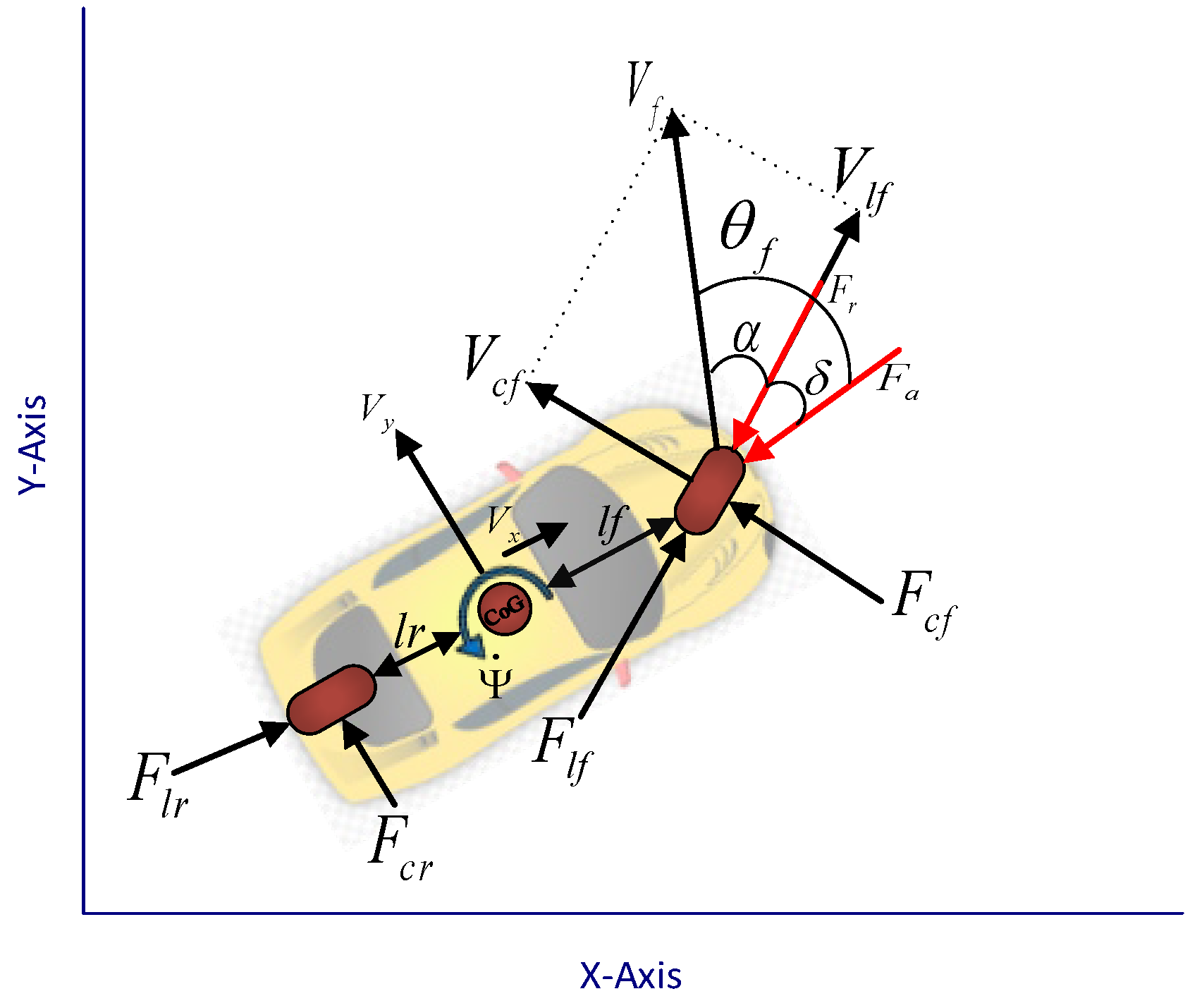
It is important to have a brief overview of the mathematical model to pave the ground for connecting the control agents later. Hence, a schematic representation of the proposed model is depicted in Figure 1. Note that $\psi$ is the yaw angle, $\dot{\psi }$ shows the yaw rate, $v_x$ and $v_y$ determines the velocity according to the vehicle coordination, $v_{lf}$ and $v_{cf}$ are the longitudinal and lateral velocity of the lead vehicle wheel, $v_f$ is their result vector, $\delta$ is the front wheel angle, and $F_l$ and $F_c$ are longitudinal and lateral wheel forces. Thus, based on Newton’s second law of motion, dynamic equations governing the system are introduced as in [28]:

$$\begin{gathered} m{\dot{v}}_x=m{\dot{v}}_y\dot{\psi }+2F_{xf}+2F_{xr} \\ m{\dot{v}}_y=-m{\dot{v}}_x\dot{\psi }+2F_{yf}+2F_{yr} \\ I\ddot{\psi }=2l_f{F}_{yf}-2l_r{F}_{yr} \end{gathered}$$

(1)

where $m$ and $I$ are the mass and inertia, $F_x$ is the lateral force, and $F_y$ is the lateral force at the center of gravity (CoG) of the vehicle. The yaw rate can be calculated as follows:

$$\dot{\psi }=\frac{v_x}{l_f+l_r}tan\left(\delta \right)$$

(2)

where ${\mathit{l}}_{\mathit{f}}$ and ${\mathit{l}}_{\mathit{r}}$ are the distances from the CoG. In addition, the position states can be obtained as:

$$\begin{gathered} \dot{X}=v_{x}cos\left(\psi \right)-v_{y}sin\left(\psi \right) \\ \dot{Y}=v_{x}sin\left(\psi \right)+v_{y}cos\left(\psi \right) \end{gathered}$$

(3)

${\mathit{F}}_{\mathit{x}}$ and ${\mathit{F}}_{\mathit{y}}$ which are the acting forces on the CoG, can be calculated by:

$$\begin{gathered} F_x=F_{l}cos\left(\delta \right)-F_{c}sin\left(\delta \right) \\ {F}_y=F_{l}sin\left(\delta \right)-F_{c}cos \end{gathered}$$

(4)

the longitudinal ${\mathit{F}}_{\mathit{l}}$ and lateral, ${\mathit{F}}_{\mathit{c}}$ forces are shown as follows:

$$\begin{gathered} F_l=f\left(\alpha ,\mu ,s,F_z\right) \\ {F}_c=f\left(\alpha ,\mu ,s,F_z\right) \end{gathered}$$

(5)

As shown in Figure 1, $\mathit{\alpha }$ is the angle between the wheel velocity vector and the wheel direction, and $\mathit{\mu }$ is the road friction coefficient. The difference between ground point velocity and the rotational velocity (slip ratio) is $\mathit{s}$, and ${\mathit{F}}_{\mathit{z}}$, which determines the vertical load action on the wheels. Under the assumption of having small $\mathit{\mu }$ values, the lateral tire forces can be obtained as:

$$\begin{gathered} F_{lf}=C_f{\alpha }_f \\ {F}_{lr}=C_r{\alpha }_r \end{gathered}$$

(6)

where ${\mathit{C}}_{\mathit{f}}$ and ${\mathit{C}}_{\mathit{r}}$ are the tire stiffness parameters and

$$\begin{gathered} {\alpha }_f=\delta -{\theta }_f \\ {\alpha }_r=-{\theta }_r \end{gathered}$$

(7)

where ${\mathit{\theta }}_{\mathit{f}}=\mathit{a}\mathit{r}\mathit{c}\mathit{t}\mathit{a}\mathit{n}\left[\frac{v_y+l_f\dot{\psi }}{v_x}\right]$ and ${\mathit{\theta }}_r=\mathit{a}\mathit{r}\mathit{c}\mathit{t}\mathit{a}\mathit{n}\left[\frac{v_y+l_r\dot{\psi }}{v_x}\right]$.

Assuming that the vehicle is traveling on flat ground, it is not affected by gravitational force but by air drag, ${\mathit{F}}_{\mathit{a}}=\frac{1}{2}{\mathit{C}}_{\mathit{D}}{\mathit{A}}_{\mathit{a}}{\mathit{\rho }}_{\mathit{a}}{\left(\mathit{v}+{\mathit{v}}_{\mathit{w}\mathit{i}\mathit{n}\mathit{d}}\right)}^2$ and rolling resistance, ${\mathit{F}}_{\mathit{r}}={\mathit{D}}_{\mathit{r}}\mathit{m}\mathit{g}\mathit{c}\mathit{o}\mathit{s}\left(\mathit{\alpha }\right)$. ${\mathit{C}}_{\mathit{D}}$ is the air drag coefficient, ${\mathit{A}}_{\mathit{a}}$ is the maximum cross-sectional area of the vehicle, ${\mathit{\rho }}_{\mathit{a}}$ is the air density, ${\mathit{v}}_{\mathit{w}\mathit{i}\mathit{n}\mathit{d}}$ is wind velocity, ${\mathit{D}}_{\mathit{r}}$ is the roll resistance coefficient, $\mathit{m}$ the vehicle mass, and $\mathit{g}$ the gravitational acceleration. For convenience, $\mathit{\alpha }$ can be ignored because ${\mathit{v}}_{\mathit{w}\mathit{i}\mathit{n}\mathit{d}}$ is very small in comparison with the vehicle velocity.

In conclusion, the equivalent dynamic state of the system can be expressed as follows:

$$\begin{gathered} \dot{X}=v_{x}cos\left(\psi \right)-v_{y}sin\left(\psi \right) \\ \dot{Y}=v_{x}sin\left(\psi \right)-v_{y}cos\left(\psi \right) \\ \dot{\psi }=\frac{v_x}{l_f+l_r}tg\left(\delta \right) \\ m\dot{v_x}=F_x+m{v}_y\dot{\psi }-2F_{cf}sin\left(\delta \right)-F_a-F_r \\ m\dot{v_y}=-m{v}_x\dot{\psi }-2(F_{cf}cos\left(\delta \right)+F_{cr}) \\ I\ddot{\psi }=2\left(l_f{F}_{cf}cos\left(\delta \right)-l_r{F}_{cr}\right) \end{gathered}$$

(8)

It should be noted that $\mathit{\delta }$ and ${\mathit{F}}_{\mathit{x}}$ are the control input of the vehicle.

3. Design of MADRL Controller

To control the AV following a lead car, velocity and distance stabilization in tracking performance of conventional methodologies like Fuzzy Logic, PID, and model predictive controller (MPC) are restricted from the following regulatory aspects:

• Since the time intervals in the simulation of vehicles are in microseconds, the computational time for designing the model-based schemes is very definitive in real-time.
• Due to the destabilization properties and high nonlinear characteristics of AVs, achieving cruise velocity and tracking control simultaneously is one of the main objectives in this field. Thus, further efforts should be considered to not only mitigate the nonlinearities effects on optimal performance control, but also ensure the stability requirements.

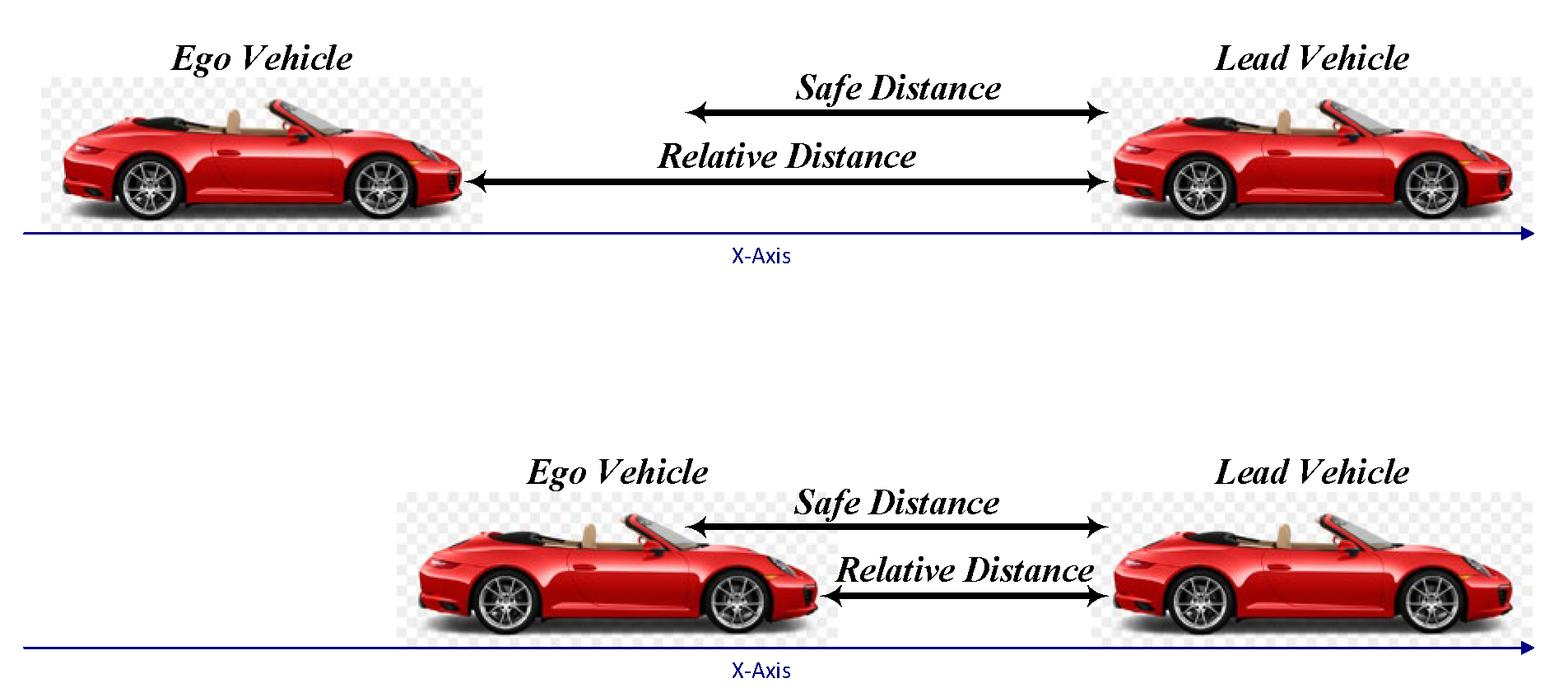
As it can be seen in Figure 2, the main control approach is to keep a safe distance and a set velocity while tracking the lead vehicle. In this case, the ego car that is tracking the lead car must follow the following rules: 1-When the distance between the ego car and the lead car is greater than a safe distance, the ego car must speed up to track the set velocity; 2-Otherwise, the acceleration must be reduced to maintain the safe distance.

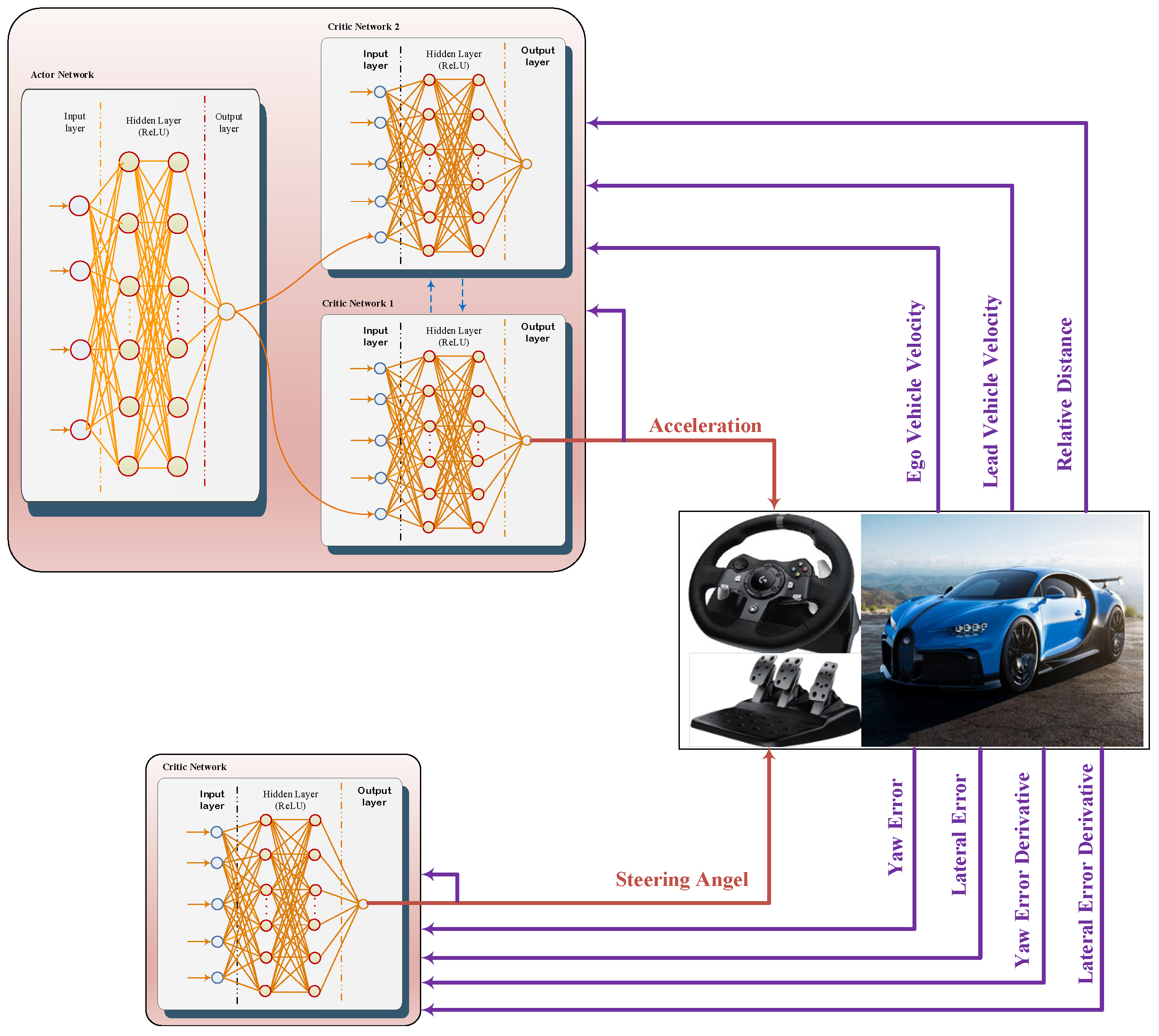
Due to the deficiency in the existing control methodologies, a MADRL-based scheme is proposed in this work in order to find a promising solution for the aforementioned challenges. Moreover, in the Multi Agent RL (MARL) algorithms, agents learn their own distinctive duties, which provides a helpful perspective on control. First, the nonlinear model of the system is employed so that sensors can be considered to identify system states and implement the suitable algorithm. Then, according to the system control inputs, the continuous agent is used for acceleration, while the discrete agent is considered for steering angle. As the acceleration force of the cars is continuous, an actor-critic model-free policy-based agent called Twin Delayed DDPG is used and compared to a DQN agent using a discrete view of acceleration. Yaw angle is set by a stepper motor, which has to be looked at completely in discrete values, and a DQN is utilized for this process.

3.1. Markov Decision Process

In the RL structure, a task can be determined by a Markov Decision Process (MDP) specified by a quintuple $\left\{S, A, r, p, \gamma \right\}$, where $S ϵ {ℝ}^n$ indicates the state space, $A ϵ {ℝ}^m$ shows the action space, $r: S\times A \to ℝ$ indicates the reward function, $p: S\times A\times S \to \left[0,1\right]$ is the transition function, which represents the probability of transiting to a new state $s_{t+1}$, emitting a reward $r$ under the execution of action $a_t$ on the state $s_t$, and $\gamma ϵ \left[0 1\right]$ indicates the discount factor. With an initial state $s_t$, the RL is aimed to maximize the obtained rewards $\mathbb{E}\left[{{\displaystyle \sum }}_{t=0}^{\infty }{\gamma }^t{r}_t \right]$.

3.2. The Twin Delayed DDPG (TD3)

A twin-delayed deep deterministic policy gradient agent is an actor-critic RL agent that calculates an optimal policy so that it optimizes the long-term reward and acts on the environment continuously. Note that the TD3 algorithm is off-policy, model-free, and an online RL technique.

The TD3 algorithm, which is an extension of the DDPG algorithm, addresses DDPG function overestimation via learning two Q-values at a time, and during policy updating, it benefits from the minimum value function. Besides, it adds noise to target actions to explore the environment more effectively. To obtain the estimation of the policy and value functions, TD3 uses the following function approximators: (1) The actor $\mu \left(S\right)$ observes the system states (or observations) and $S$ correspondingly acts on the environment in a way that maximizes the long-term reward. (2) To increase the stability of the optimization process, the agent ${\mu }^{\prime }\left(S\right)$ regularly updates the target actor parameters using the received values. (3) State set $S$ and action set $A$ input to the critics, then they give the related expectation of the long-term reward. (4) The previous procedure is periodically done at a determined time to update the target critics. The critics should follow the same structures, but their corresponding targets have to be the same. For better understanding, Figure 3 demonstrates the TD3 algorithm in detail.

4. MADRL AV TD3 Agent for Acceleration Control

Based on the knowledge of the AVs sensors outputs, the exact observations and reward function could be defined. Figure 4 shows that the observation and reward function consist of four parameters: (1) Relative distance (the difference between the lead and ego vehicles positions); (2) Lead vehicle velocity; (3) Ego vehicle velocity; and (4) Last exerted acceleration. It is important to explicitly address a series of calculations before dealing with observations. To do so, the safe distance between the lead car and the ego car, $D_{safe}$, is defined as:

$$D_{safe}=D_{default}+T_{gap}{V}_{ego}$$

(9)

where $D_{default}$ is the pause default distance in meters,$T_{gap}$ shows the time gap between the vehicles in seconds, and $V_{ego}$ defines the ego vehicle velocity. The error distance is

$$D_{error}=D_{safe}-D_{rel}$$

(10)

One should bear in mind that the velocity error is another significant issue, which can be calculated as follows:

$$V_{\mathit{error}}=\{\begin{array}{c}\min \left\{V_{lead}, V_{set}\right\}-V_{ego} if \min \left\{V_{lead}, V_{set}\right\}\\ V_{set}- V_{ego} otherwise\end{array}$$

(11)

where $V_{lead}$ is the lead vehicle’s velocity, and $V_{set}$ is the velocity at which the ego vehicle is set to drive. Therefore, the observation would be defined as $\left\{V_{error},\int V_{error}, V_{lead}\right\}$.

To compose the reward function, the first step is to calculate the cost function. The cost function consists of the consumed energy, the control action, and the error in velocity with different weights. The cost function is defined as:

$$Cost function1=\sum w_1{V}_{error}^2+w_2{F}_x^2$$

(12)

where ${\mathit{w}}_{\mathbf{1}}$ and ${\mathit{w}}_{\mathbf{2}}$ are the weights of the considered values, and ${\mathit{F}}_{\mathit{x}}$ (or $\mathit{a}$) is the acceleration. The reward function, which is expected to be maximized in the training process, is defined as the minus of the cost function. Throughout this study, the actor-critic TD3 consists of two fully connected hidden layers (HLs) with 50 neurons for both the actor and critic structures. The “rectified linear unit (ReLU)” activation function is applied to all HLs in the network. Readers are directed toward Figure 5 for a schematic configuration representation of the MADRL AV. Additionally, the parameters for the implemented algorithm are given in

Table 1. Parameters of the TD3 agent.

Parameter	Value	Parameter	Value
TD3 Training Episode Length	500 ts	Critic2 Learning Rate	1 × 10−3
Minimum Batch Size	1024	Number of MC cycle	200
Actor Learning Rate	1 × 10−4	Discount Factor	0.99
Crtitic1 Learning Rate	1 × 10−3

.

5. Deep-Q-Network (DQN)

A DQN agent is an off-policy, value-based RL agent that acts on the environment discretely. Moreover, the DQN algorithm is a model-free, online RL technique. It is challenging in complex state-action spaces to learn from the evaluation of the $Q$ value of both state and action separately. In DRL, several agents’ parts, such as policy $\mathsf{\Pi }\left(\mathrm{s},\mathrm{a}\right)$ or values $q\left(s,a\right)$ are given with deep NNs. These NNs parameters are trained to minimize some loss functions through the gradient descent method. In DQN, deep networks and RL estimate values from NNs and the given states $S_t$. In each step, based on the current state, the agent chooses an action based on the action values $ϵ-greedily$ and the data $\left(S_t,A_t,R_{t+1},{\gamma }_{t+1},S_{t+1}\right)$ which have all the preceding data in time $t$. NNs parameters are then trained using random gradient descent to minimize the following loss function:

$${\left(R_{t+1}+{\gamma }_{t+1}\underset{a^{\prime }}{max}{q}_{\theta }\left(S_{t+1},a^{\prime }\right)-q_{\theta }\left(S_t,A_t\right)\right)}^2$$

(13)

where $t$ is the time step. The cost function gradient for updating$\theta$ is done via the back-propagation method. $\theta$ defines the target network’s parameters and is a copy of the online network over a given time period. Optimization is performed using RMSprop on small, sampled batches from replay memory. The structure of the DQN algorithm is shown in Figure 4.

6. The MADRL AV DQN Agent for Steering Angle Control

Similarly, as defined in the observations and reward function for TD3, for the purpose of having control over the steering angle, some calculations should be done for the DQN agent. As shown in Figure 5, the agent receives some inputs from the environment, including: 1-${\dot{L}}_{error}$(Lateral error derivative); 2-${\dot{Y}}_{error}$ (Yaw error derivative); 3-$L_{error}$ (Lateral error); 4-, $Y_{error}$ (Yaw error); and 5- $\theta$ (Steering angle). Next, the observation set can be calculated as $\left\{L_{error} , {\dot{L}}_{error}, \int L_{error}, Y_{error}, {\dot{Y}}_{error}, \int Y_{error}\right\}$. To obtain the corresponding reward function, first the cost function should be calculated as follows:

$$Cost function2=\sum {w^{\prime }}_1{L}_{error}^2+{w^{\prime }}_2{\theta }^2$$

(14)

where ${w^{\prime }}_1$ and ${w^{\prime }}_2$ are weights of the considered values, and $\theta$ is the steering angle. The reward function, which is expected to be maximized in the training process, is defined as the minus of the cost function.

In this work, similar to TD3 in part $C$, DQN consists of two fully connected HLs with 50 neurons. For all HLs in the network, the ReLU activation function is used. The configuration is specified in the lower agent of Figure 5, and the parameters for the implemented algorithm are provided in

Table 2. Parameters of the DQN agent.

Parameter	Value	Parameter	Value
DQN Training Episode Length	500 ts	Number of MC Cycle	500
Minimum Batch Size	1024	Discount Factor	0.99
Learning Rate	1 × 10−3

.

7. Results and Discussion

In this section, we evaluate the effectiveness of our proposed multi-agent DRL-based control technique and compare it to two of the state-of-the-art control alternatives, namely Holistic Adaptive Multi-Model Predictive Control (HMPC) and Hierarchical Predictive Control (HPC). HMPC [29] has a linear structure, which makes it perform well in real-time. It also has a weight-adaptive mechanism to improve its handling ability and a multi-model adaptive law to account for tire cornering stiffness uncertainties. HMPC benefits from a weight-adaptive structure to control the system in uncertain situation. HPC [30] provides a structure to switch between multiple model predictive controllers in order to decrease the response time. HPC switches between the models at runtime based on a metric called uncontrollable divergence, which reveals the divergence between predicted and true states caused by return time and model mismatch. The relevant parameters of the AV are given in

Table 3. Parameters used in the vehicle model.

Parameter	Abbreviation	Value
Vehicle mass	$m$	$1500\mathrm{kg}$
Inertia around z-axis	$I$	$1300{\mathrm{mNs}}^2$
Cornering stiffness front wheels	$C_f$	$13,000\mathrm{N}/\mathrm{rad}$
Cornering stiffness rear wheels	$C_r$	$12,500\mathrm{N}/\mathrm{rad}$
Distance from front wheels to CoG	$l_f$	$\mathrm{m}$
Distance from rear wheels to CoG	$l_r$	$\mathrm{m}$
Cross sectional area	$A_a$	$10.25{\mathrm{m}}^2$
Roll resistance coefficient	$D_r$	1.5 × 10−3
Air drag coefficient	$C_D$	0.6
Air density	${\rho }_A$	$1.3\mathrm{kg}/{\mathrm{m}}^3$
default spacing between lead and ego cars	$D_{default}$	$\mathrm{m}$
time gap for distance maintaining	$t_{gap}$	1.5 s
set velocity for ego car	$V_{set}$	$30\mathrm{m}/\mathrm{s}$

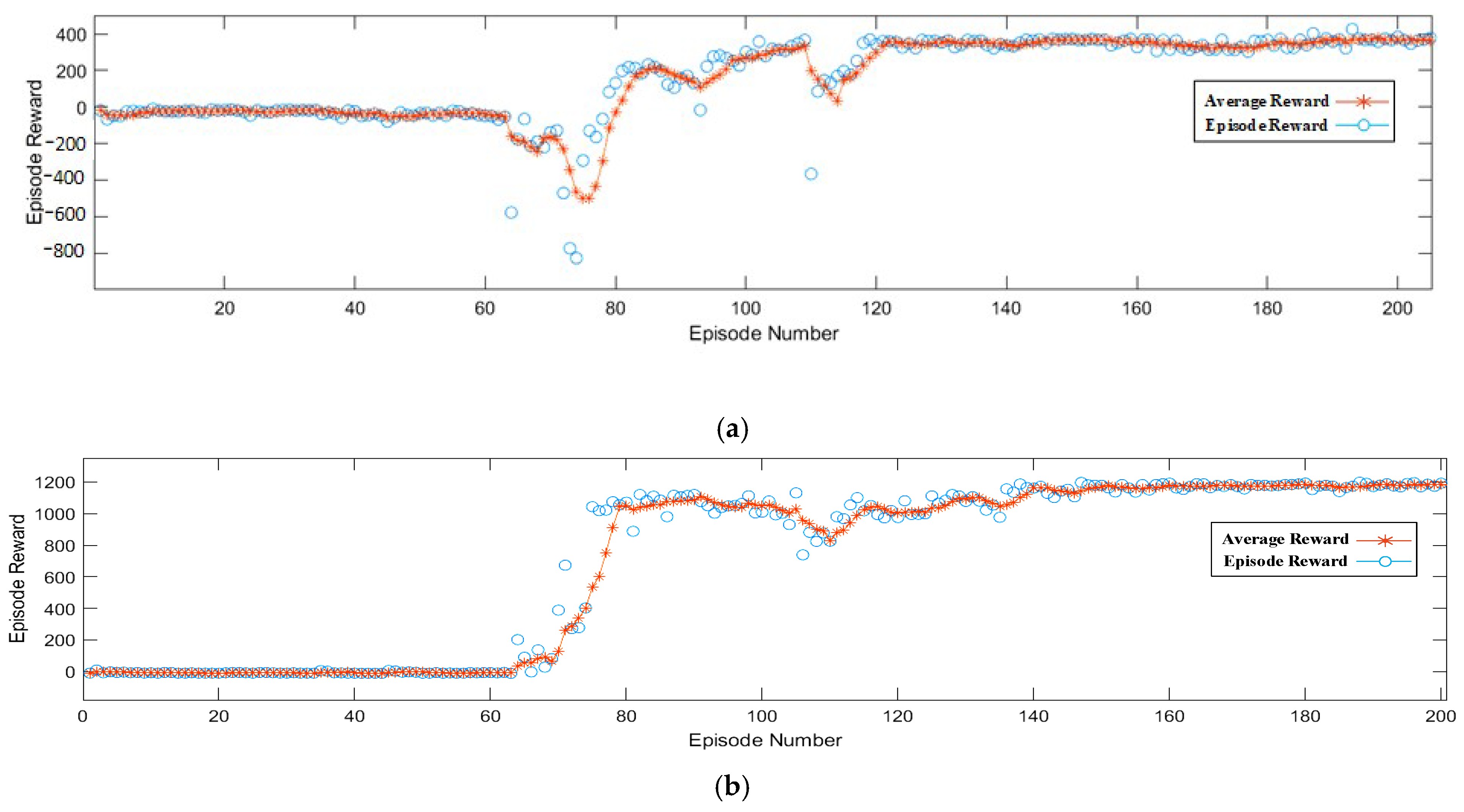
. In this application, to investigate the reliability and effectiveness of the proposed MADRL controller, the errors of yaw angle, lateral distance error, distance, velocities, and control efforts are investigated. The iterations in which the agents are trained are studied too. Figure 6a plots the training reward against the number of completed epochs. As seen, the training reward improves with every epoch, indicating the algorithm’s gradual learning and performance enhancement.

To visualize the trend better, Figure 6b also shows the same training progress with an added trendline, which displays a clear improvement in the training reward over time, affirming the algorithm’s successful learning and performance enhancement.

As shown in Figure 6a,b, our MADRL based controller outperforms in stabilizing the system under favorable conditions of tracking the lead vehicle at a set velocity and avoiding crossing the safety distance. The progress depicted in Figure 6a,b resulted from the execution of our proposed algorithm on the training data, which was done through multiple epochs. Every epoch entailed iterating through the data set and adjusting the algorithm based on the feedback from the training reward.

The training reward is a metric that reflects the algorithm’s performance during training, which is determined by a specific objective function. This function aims to minimize the error between the algorithm’s predicted and actual outputs, and it gauges the degree to which the algorithm is learning and enhancing its performance.

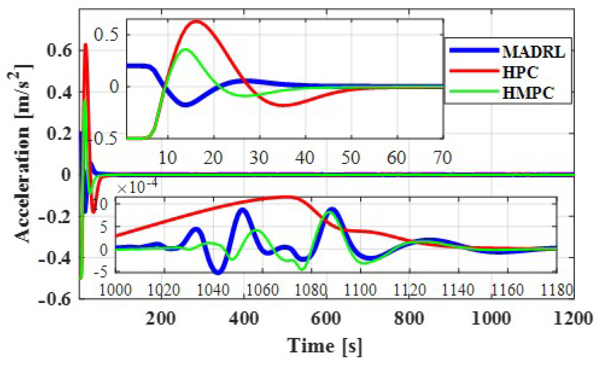
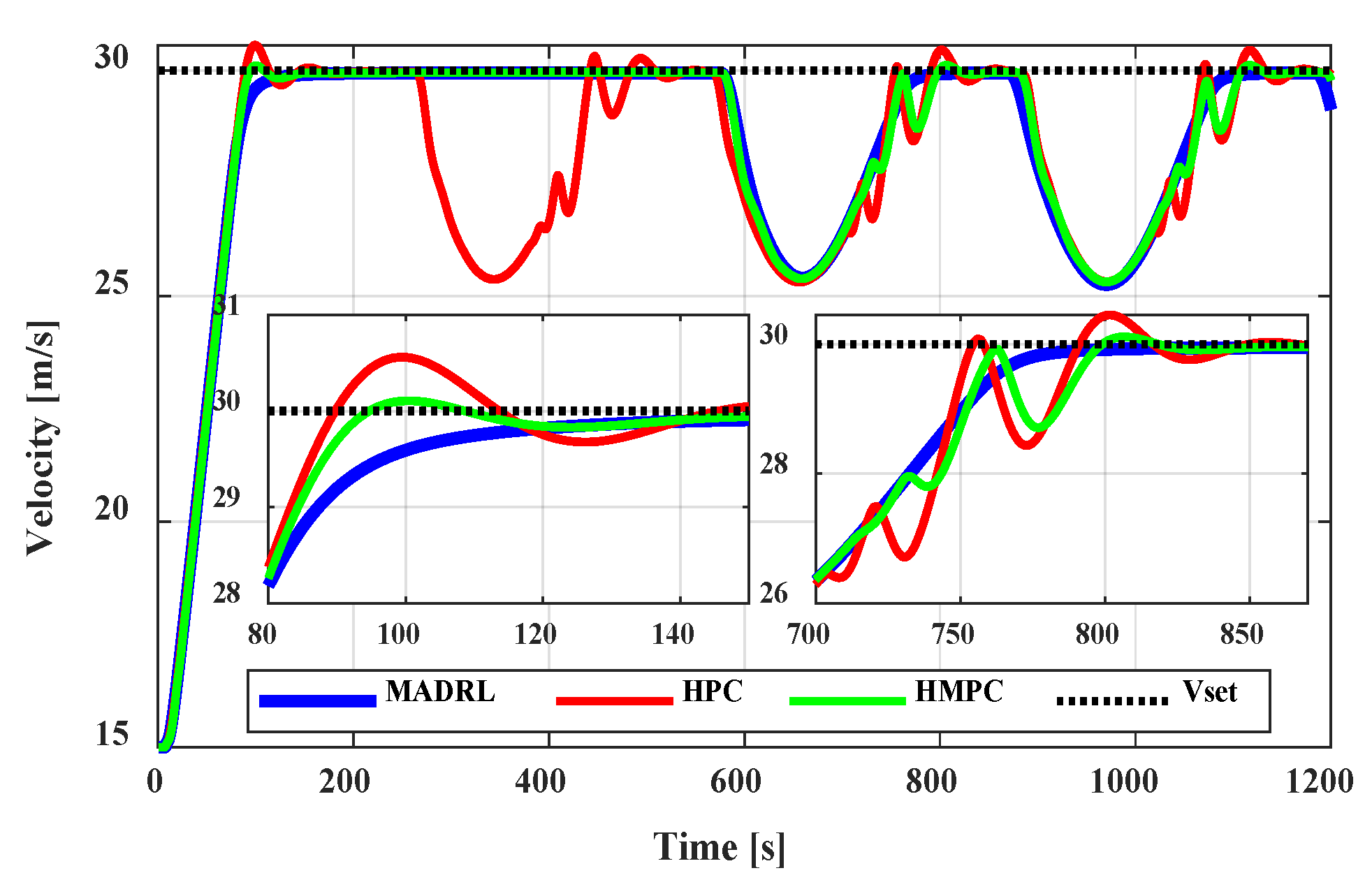
To achieve this, as presented in Figure 7, in the early stages of driving to maintain a safe distance, the accelerations fluctuate sharply, and the range of acceleration decreases over time. In the MADRL algorithm, to achieve the set speed, the controller starts moving at a relatively high acceleration and reduces its acceleration smoothly over time, but in the two HPC and HMPC algorithms, the vehicle accelerates after about 7 s. In the velocity diagram, the MADRL method clearly proves its superiority over the two HPC and HMPC algorithms. 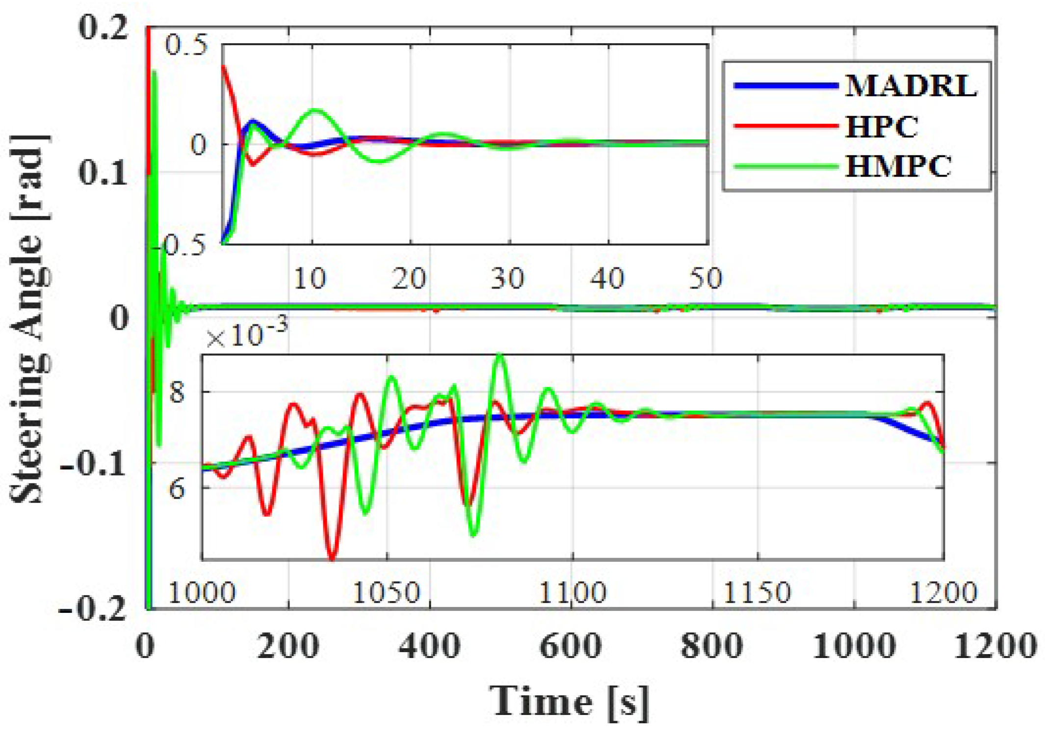It can be seen in Figure 8 that the two alternative algorithms can track a velocity of 30 m/s with overshoots along with some fluctuations. However, the trained neural network with MADRL controls the velocity in the way that it benefits both smooth tracking behavior and fast settling time. This optimized behavior of the system with MADRL in steering angle changes is also shown in Figure 9, while HPC and HMPC methods show oscillating behavior that is not practical and not useful as they definitely cause destructive damages to passengers. In all three compared algorithms, the need to maintain the distances between the two vehicles is another significant issue that should be investigated. 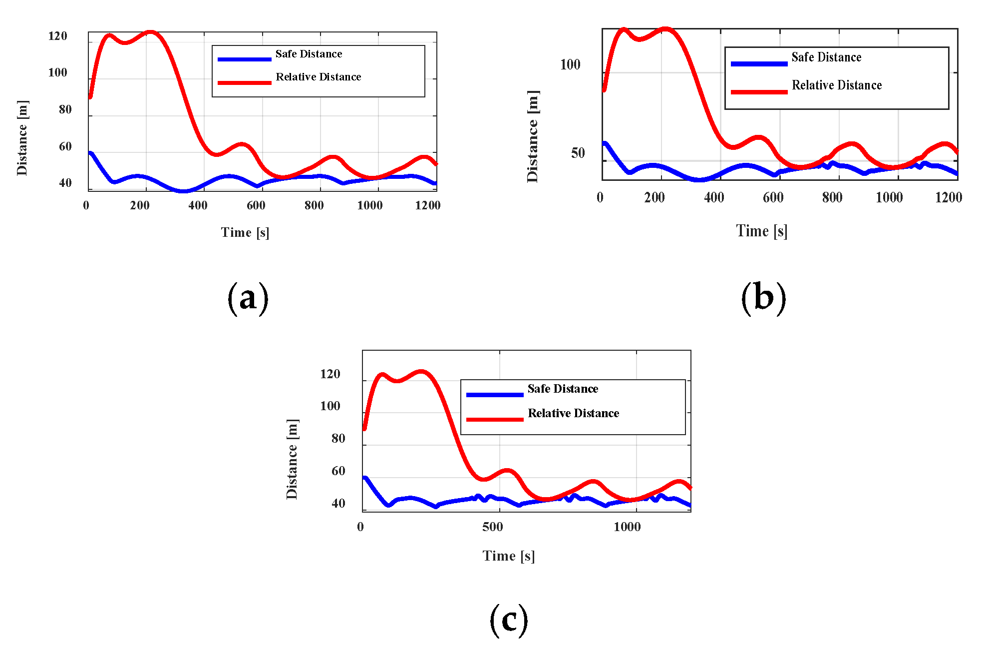Figure 10a–c represents the relative and safe distances of the ego and lead vehicles when MADRL is applied. By adjusting the speed with acceleration, the ego vehicle keeps its distance from the lead vehicle in a way not to cross the safe distance, while sustaining a relative distance to be able to follow it properly. The HPC and HMPC algorithms are shown in Figure 10b,c and they follow the same principle formulated in their constraints in the optimal control problem. 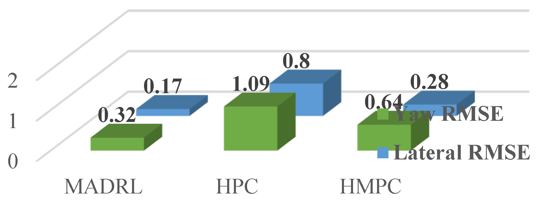As it is obvious in Figure 10a, compared to Figure 10b,c, the safe distance diagram benefits from a smooth behavior, while the HPC and HMPC algorithms experience some oscillating behaviors, for example, at times of 750 and 1080 s for HPC and at times of 420, 760, and 1080 s for HMPC. It can be perceived that with path following and cruise control, all the controllers work in the right way to keep a safe distance and track the trajectory of the leading vehicle. Moreover, the root mean square error (RMSE) is also studied for three algorithms for steering and lateral distance, as depicted in Figure 11. It is evident that the lowest RMSE is obtained using our MADRL controller. As a result, it can be readily seen that the MADRL outperforms the two state-of-the-art algorithms considered earlier.

8. Conclusions

This paper proposes a multi-agent deep reinforcement learning-based method to control both speed and steering (cruise control) of unmanned vehicles using DLR agents, in which the agents learn to select the optimum actions to control steering and acceleration. The proposed method has the potential to enhance the safety and efficiency of autonomous vehicles, particularly in challenging environments due to its reduced computation requirements distributed among agents. The study’s findings reveal that the suggested approach surpasses existing state-of-the-art techniques, demonstrating its potential to be applied in real-world situations. To overcome the real-time learning mission, both the DQN and TD3 for the actor and critic sections follow the structure of two hidden layers made up of 50 neurons, with the RELU acting as the activation function. To meet the control requirements, the MADRL technique was used, where one agent is in charge of acceleration and the other is considered to be steering angle. As a result, the following outcomes were obtained: 1-yaw and lateral errors reached approximately zero in less than 4 s, 2-the ego’s velocity reached set point velocity in less than 10 s, while it is intelligent not to pass the safe distance simultaneously, 3-acceleration and steering act in such a way that the smallest amount of energy was acquired. Lastly, the performance of the proposed control method was tested and compared to two state-of-the-art techniques, HPC and HMPC, with the clear outcome that our proposal outperforms the state-of-the-art techniques. A future work would be to consider other challenges and risks related to delays, data loss, and control compromise of AV and propose new mitigation agents to maintain safety.