Article

Enhanced Round-Robin Algorithm in the Cloud Computing Environment for Optimal Task Scheduling

by
Fahd Alhaidari
1,* and
Taghreed Zayed Balharith
2
1
Networks and Communications Department, College of Computer Science and Information Technology, Imam Abdulrahman Bin Faisal University, P.O. Box 1982, Dammam 31441, Saudi Arabia
2
Computer Science Department, College of Science and Humanities, Imam Abdulrahman Bin Faisal University, P.O. Box 12020, Jubail 31961, Saudi Arabia
*
Author to whom correspondence should be addressed.
Computers 2021, 10(5), 63; https://doi.org/10.3390/computers10050063
Submission received: 6 April 2021 / Revised: 3 May 2021 / Accepted: 5 May 2021 / Published: 9 May 2021

Abstract

:
Recently, there has been significant growth in the popularity of cloud computing systems. One of the main issues in building cloud computing systems is task scheduling. It plays a critical role in achieving high-level performance and outstanding throughput by having the greatest benefit from the resources. Therefore, enhancing task scheduling algorithms will enhance the QoS, thus leading to more sustainability of cloud computing systems. This paper introduces a novel technique called the dynamic round-robin heuristic algorithm (DRRHA) by utilizing the round-robin algorithm and tuning its time quantum in a dynamic manner based on the mean of the time quantum. Moreover, we applied the remaining burst time of the task as a factor to decide the continuity of executing the task during the current round. The experimental results obtained using the CloudSim Plus tool showed that the DRRHA significantly outperformed the competition in terms of the average waiting time, turnaround time, and response time compared with several studied algorithms, including IRRVQ, dynamic time slice round-robin, improved RR, and SRDQ algorithms.

1. Introduction

Cloud computing has become a buzzword in today’s IT industry, where it is one of the essential modern trends that has caused a fundamental change in this area. In a cloud computing environment, technology is introduced in the form of services. It allows the use of servers, storage, and applications at any time by using different types of computers or smartphones securely and at the lowest cost [1].
Cloud computing can be identified as Internet-based computing that provides a pool of adaptable computing resources, including networks, storage, servers, applications, and services without a need to interact with the service provider and with the minimum management effort. Moreover, customers are supplied with resources in the form of different service models. The resources can be infrastructure as a service model (IaaS), a platform as a service model (PaaS), or software as a service model (SaaS) [2].
One of the critical research issues in a cloud computing environment is task scheduling. With the increasing number of cloud users, sufficient access to remote resources and maximum profit are two of the main objectives of service providers. Task scheduling is the technique used for mapping clients’ tasks to the available and appropriate virtualized resources by using an efficient algorithm [3]. In heterogeneous computing such as cloud computing, the issue of task scheduling becomes more challenging since it is a distributed and scalable environment. Therefore, there is a need for an effective task scheduling algorithm, which is considered key for the performance of the system [3,4,5].
In a cloud computing environment, there are three common categories of task scheduling algorithms [6], which are (1) traditional algorithms, such as first come first serve (FCFS), shortest job first (SJF), largest job first (LJF), and round-robin (RR) [7], (2) heuristic algorithms, such as Min-Min and Max-Min algorithms [8], and (3) meta-heuristic algorithms, such as the ant colony optimization algorithm (ACO) [9] and particle swarm optimization (PSO) [10].
The round-robin (RR) algorithm is one of the most commonly used scheduling traditional algorithms. It is simple and depends on sharing CPU time [11,12]. In the RR algorithm, the jobs share the CPU time by allocating a slice of time, usually between 10 and 100 ms for each job, called quantum time (QT) [13]. If the current job is over, its execution will be paused, and it will be placed at the end of the ready queue. These steps are repeated for all jobs in the ready queue. If the job’s execution is completed, it will be deleted directly from the ready queue. It is obvious from the above discussion that the efficiency of the RR algorithm depends on the QT, and therefore, the choice of the QT size is a critical issue for improving the overall performance of the RR algorithm. If the QT size is too large, RR tends to become an FCFS algorithm, whereas if the QT is too small, RR might perform poorly due to the context switches that cause much overhead [14]. Algorithm 1 shows the pseudocode of the RR algorithm as described in [15].
Algorithm 1 The Pseudocode of the RR Algorithm in CPU Scheduling [15]
Step 1: Keep the ready queue as a FIFO queue of tasks
Step 2: New tasks added to the tail of the queue will be selected, set a timer to interrupt after one time slot, and dispatch the tasks.
Step 3: The task may have executed less than one time quantum. In this case:
  •  The task itself will release the resources voluntarily;
  •  The scheduler will then proceed to the next task in the ready queue.
Step 4: Otherwise, if the running task is longer than one time quantum,
  the timer will go off and will cause an interruption to the OS.
The main contribution of this paper is to propose a novel technique focusing on the traditional RR algorithm disadvantages. The proposed model optimizes the functionality of the traditional RR algorithm for scheduling tasks in the cloud computing environment through optimizing the performance metrics by decreasing the average waiting time, average turnaround time, and average response time.
The rest of this paper is organized as follows. In Section 2, the literature review is presented. In Section 3, the problem statement is illustrated, while the proposed technique is explained in detail in Section 4. Section 5 presents the simulation setting, and Section 6 comprises the evaluation and discussion. Finally, the conclusion and future work are discussed in Section 7 and Section 8, respectively.

2. Literature Review

Since the selection of quantum time is an important issue affecting the RR algorithm’s efficiency, many researchers have conducted several studies to improve its efficiency by proposing various techniques to calculate the optimal quantum time.
In [14], the authors presented a survey on studies related to enhancing the RR algorithm. We found that some researchers improved the RR algorithm by considering a fixed quantum time, while other studies proposed improving the performance of the RR algorithm by calculating a dynamic quantum time, which may be dynamic in each round or for each task.
In [16], the authors proposed a novel approach to improving the RR algorithm, relying on the median burst time of the ready queue tasks. These tasks should be sorted in ascending order at the beginning. Then, tasks will be divided into two subqueues: light and heavy task queues. The tasks are rearranged after each round based on the remaining burst time. In each round, the quantum time is equal to the burst time for the medium task. This approach has proven its effectiveness in reducing the waiting time and turnaround time compared with the traditional RR and IRRVQ algorithms.
In [17], the researchers proposed a new approach named the eighty-five percentile RR algorithm (EFPRR). It is based on computing a TQ using 85% of the burst time of the tasks. The processes are initially arranged in incremental order based on their burst time, and then the TQ is calculated by multiplying the average time of all tasks by the 85% constant (85% average). Then, the remainder of the BT for the tasks is checked. If it is less than or equal to the TQ, the running tasks are executed until completion. Otherwise, the tasks are relocated at the tail of the ready queue. The EFPRR was evaluated through several experiments, showing the effectiveness of the proposed algorithm in reducing the average burst times.
In [18], the authors developed a new mechanism to calculate the quantum time in the RR algorithm based on the average burst time of all ready queue tasks. The SJF is applied initially, and then the quantum time is calculated for the first round. This calculation is repeated every round as new tasks enter the ready queue. The results showed an enhancement of the RR algorithm by reducing the average waiting time, average turnaround time, and the number of context switches (CSs). Similarly, the authors in [19] proposed a new technique to calculate the quantum time in the RR algorithm. The tasks should be located in the ready queue as they arrived. Then, the QT will be calculated based on the average of the tasks’ burst time. The evaluation experiments showed the efficiency of the new technique in reducing the waiting time and turnaround time.
In [20], the authors suggested improving the RR algorithm based on an analytic model that considers several parameters, such as the execution time and the task order. The improved model was evaluated by conducting several different scenarios. These experiments proved the model’s effectiveness in improving the average waiting time and average response time. Similarly, in [21], the authors proposed improving the RR algorithm by using a dynamic time quantum, which was calculated using a mathematical equation based on the median of the tasks’ burst time and the smallest burst time in the ready queue. The efficiency of the improved RR was investigated by a comparison with the traditional RR algorithm. The results showed the efficiency of the improved algorithm in terms of the maximum CPU utilization, throughput, and minimized waiting time, response time, and the number of context switches.
In [22], the authors proposed a new approach to enhancing the RR algorithm, where the quantum time was determined by computing the maximum difference among the differences of adjacent consecutive processes in the ready queue. The results showed an improvement in the system performance due to reducing the average turnaround time, average waiting time, and the number of context switches.
In [23], the authors proposed a combination of SJF and RR algorithms to improve the performance of the RR algorithm. The main idea in their proposed technique was to distribute the presented tasks into two queues, where the median was used as a threshold for distributing the tasks among the two queues. The results of the experiments showed the success of this algorithm in reducing both the waiting time and response time.
In [24,25], the authors proposed an enhancement to the dynamic RR algorithm, tuning the quantum time by assigning a value for the quantum time equal to the average of the burst time of the tasks in the ready queue. On other hand, in [26], the authors proposed assigning the average of the burst time for the quantum time, but by applying the remaining burst time principle [27]. This principle states that if the remaining burst time of the task is less than the quantum time, the task completes its execution and then exits the ready queue.

3. Problem Statement Gap Analysis

To identify the main gap and shortages with the proposed algorithms discussed in the literature review, we studied the behavior of the algorithm in [26] by considering the three datasets used in [26], which involve tasks with a different burst time order but an arrival time equal to zero. Table 1 shows samples from such a dataset with numerical values to reflect the properties of them.
Figure 1 presents an analytical study considering the following cases: (1) the behavior of the proposed dynamic round-robin (DRR) algorithm discussed in [26], (2) the behavior of the same algorithm when it is integrated with FCFS, and (3) the behavior of the same algorithm when it is integrated with SJF. Finally, a comparison with the traditional algorithms including both FCFS and SJF is made.
It can be observed from Figure 1 that if the quantum time equals the average of the tasks’ burst time and the RR algorithm applied the remaining burst time principle, there are two cases as follows. The first case is when the same order of tasks is maintained; in other words, the RR algorithm is integrated with the FCFS algorithm. The second case is when the RR algorithm is integrated with SJF. In the first case, it is obvious that the RR algorithm tends to be FCFS with the same average waiting, turnaround, and response times. Moreover, the CS number is equal to the number of tasks, which means that each task is allocated the CPU one time and is executed during its own burst time. Similarly, for the second case, it is clear that the RR algorithm tends to be SJF with the same average waiting, turnaround, and response times. Moreover, the CS number is equal to the number of tasks, which means that each task is allocated the CPU one time and is executed during its own burst time.
From the above conducted analysis, it can be concluded that applying the concept of the remaining burst time on the dynamic RR algorithm, where the QT is equal to the average of the tasks’ burst time, is not efficient. Moreover, in this way, the RR algorithm loses its nature. Thus, this paper introduces a novel technique named the dynamic round-robin heuristic algorithm (DRRHA), which concentrates on providing a solution for the time quantum problem by tuning the time quantum dynamically for each presented task in the ready queue based on its burst time. Moreover, we introduce the utilization of the advantages of the STF algorithm to improve the performance of the proposed model [28]. This novel technique will be discussed in detail in the next section.

4. The Proposed Technique

In our proposed DRRHA approach, presented in Figure 2, the tasks are initially received from the users and stored in the ready queue according to their order of arrival (FCFS). Then, each task arrives at the ready queue and is sorted based on the SJF manner. In each round, the average mean is calculated for all the tasks in the ready queue. After that, the quantum time is calculated for each task separately according to Equation (1). If the remaining burst time is less than or equal to its quantum, then the task execution is completed, and it is removed from the ready queue. Otherwise, the task is stored at the end of the ready queue and is to be executed in the next round. Moreover, if new tasks arrive, they are stored in the ready queue until the current round is finished:
Q T i j = ( m 2 ) + ( m 2 ) B T i j   ,
where Q T i j is the quantum time of task i in round j, m is the average mean at the ready queue, and B T i j is the burst time or the remaining burst time for task i in round j.
The DRRHA is composed of seven main steps and they are as follows:
Step 1: Arrange the submitted tasks in ascending order based on their burst time.
Step 2: Compute the arithmetic mean for all tasks in the ready queue.
Step 3: Calculate the value of the time quantum based on Equation (1).
Step 4: Execute all tasks based on their calculated time quantum.
If the task finishes its time quantum, there are two cases:
Step 4.1: If the remaining burst time is less than or equal to its time quantum, complete its execution. Then, remove this task from the ready queue.
Step 4.2: If the remaining burst time of the task is greater than its time quantum, pause the task and insert it into the tail of the ready queue.
Step 5: When a new task arrives, do the following:
  • Sort all tasks in the ready queue in the STF manner.
  • The m and Q T i j values for all the tasks in the ready queue will be recalculated.
Step 6: When a task is finished, the m and Q T i j values for all the tasks in the ready queue will be recalculated.
Step 7: Repeat all the steps until all the tasks are finished.
The details of the main steps involved in the proposed approach are shown in Algorithm 2. Moreover, Figure 3 shows a flowchart describing the followed procedure of the proposed approach.
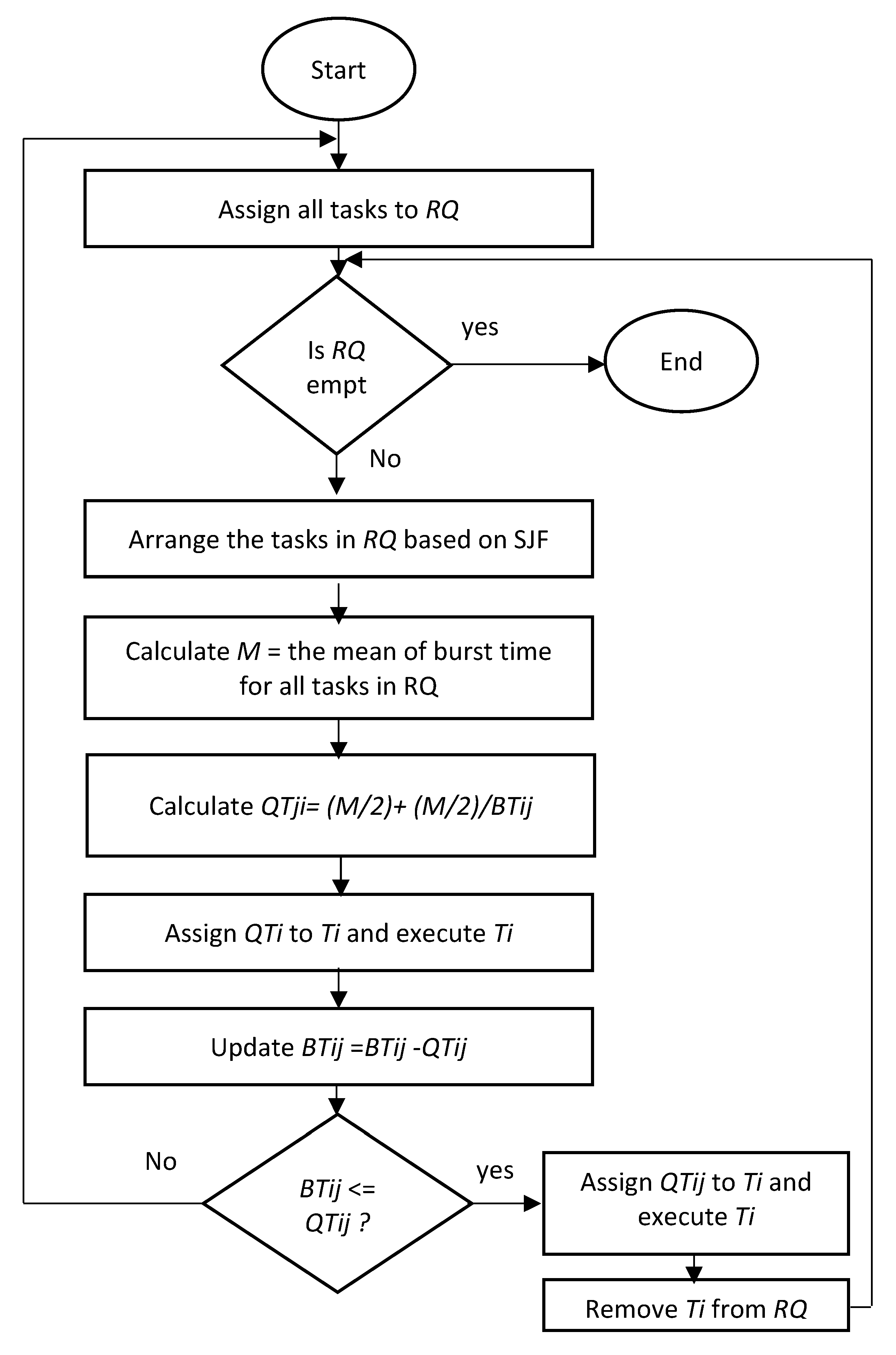
Algorithm 2 Proposed DRRHA
Declarations
Ti: Task i
BTij: Burst time or the remaining burst time of task i in the round j
RQ: Ready Queue
Count_Iteration: an initialized value for iteration j and Quantum Time QTij
M: The arithmetic mean of burst time of tasks.
QTij: Quantum time assigned to task, Ti, in the round j
Input: Tasks, Ti
Output: Rescheduling all tasks, Ti
BEGIN
 Submitted tasks in RQ based on arrival time.
WHILE (RQ is not empty)
BEGIN
  Arrange all arrived tasks in RQ based on SJF
  M = The mean of burst time of the tasks that arrived in RQ.
  For (each task Ti in RQ)
  BEGIN
   QTij = (M/2) + (M/2)/BTij
   Execute (Ti)
   BTij = BTijQTij
   IF (BTij < QTij): Execute (Ti) again
   Else: Add Ti at the end of RQ
   IF (BTij (Ti) = 0)
   BEGIN
    Remove (Ti) from RQ
    M = The mean of burst time of the remaining tasks in the RQ.
    For (each task Ti in RQ): QTij = (M/2) + (M/2)/BTij
   End IF
   IF (a new task is arrived)
   BEGIN
    Sort all tasks in RQ based on SJF
    M = The mean of burst time of all tasks in the RQ.
    For (each task Ti in RQ): QTij = (M/2) + (M/2)/BTij
   End IF
  j++
END FOR
 END WHILE
END

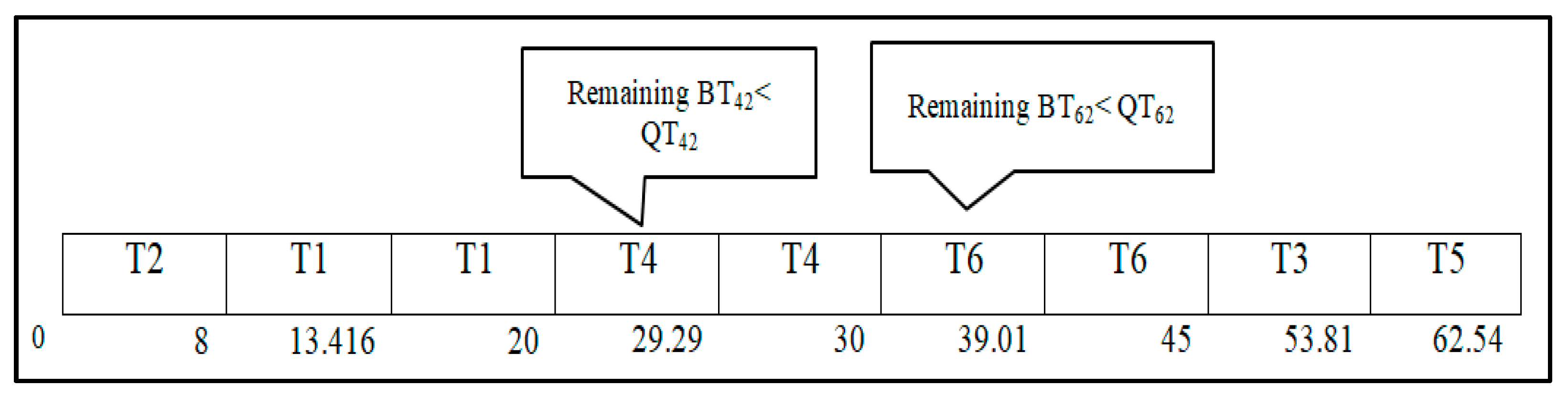
Case Study: The Impact of Integrating the Proposed Model (DRRHA) with the SJF Algorithm

Here, we consider a case of six tasks with non-zero arrival times, as shown in Table 2.
The following are the detailed steps for the proposed technique (DRRHA) with the SJF algorithm.
(1)
Round 1
After the arrival of tasks T1 and T2, these tasks were arranged in ascending order based on the burst time. Then, the QT for each task was calculated as illustrated in Table 3. After that, these tasks were scheduled as shown in Figure 4.
(2)
Round 2
In this round, tasks T3, T4, T5, and T6 arrived and were added into the head of the RQ, which contained task T1 from the previous round. Then, all tasks in the RQ were arranged in ascending order based on their burst time as shown in Table 4. After that, the QT was calculated for each task separately as presented in Table 5. Finally, these tasks were scheduled and executed as shown in Figure 5.
(3)
Round 3
In this round, the remaining tasks in the RQ should be rearranged in ascending order based on their burst time as shown in Table 6. Then, the QT for each task was calculated as illustrated in Table 7. Finally, these tasks were rescheduled and executed as shown in Figure 6.
Table 8 shows the evaluation results of the case study presented in this section, where it shows the overall statistic of the scenario in terms of the waiting time (WT), turnaround time (TAT), and response time (RT).

5. Simulation Settings

The proposed DRRHA technique was implemented and tested in the CloudSim Plus environment [29], which is an extensible and fully featured simulation framework. It is based on the CloudSim framework and allows cloud computing infrastructure and application services to be modeled, simulated, and tested. The main reason for choosing this simulation tool was because it has the capacity for integrated modeling and evaluates application services. It supports task scheduling policies, virtual machine (VM) selection, setting the network connections, locating energy models for the resources of data centers, and supplying various forms of workloads [29,30].
Table 9 summarizes the simulation settings used in the CloudSim Plus experiments for testing our proposed approach. NetBeans IDE8.2 was used as an environment to run the CloudSim libraries.

6. Evaluation and Discussion

The performance of the proposed DRRHA technique was evaluated considering the following four performance metrics [31]: (1) waiting time, or the total time tasks spent in the ready queue; (2) response time, being the time elapsed from the arrival of the task until starting its execution; (3) turnaround time, which was the time elapsed from the arrival of the task until completing its execution; and (4) context switches, or the number of times that the task status changed from one activity to another.
We considered three different scenarios to evaluate the proposed model as follows:
(1)
Evaluating the proposed model by comparing it with SJF and FCFS algorithms to study the impact of integrating the proposed model with these algorithms;
(2)
Comparing the proposed model with the related algorithms from the literature review;
(3)
Evaluating the performance of the proposed model using two datasets: a real dataset and a randomly generated dataset.
Moreover, for each experiment, the improvement rate of the proposed algorithm was measured by calculating the difference between the proposed algorithm and the considered algorithm for all the performance metrics.

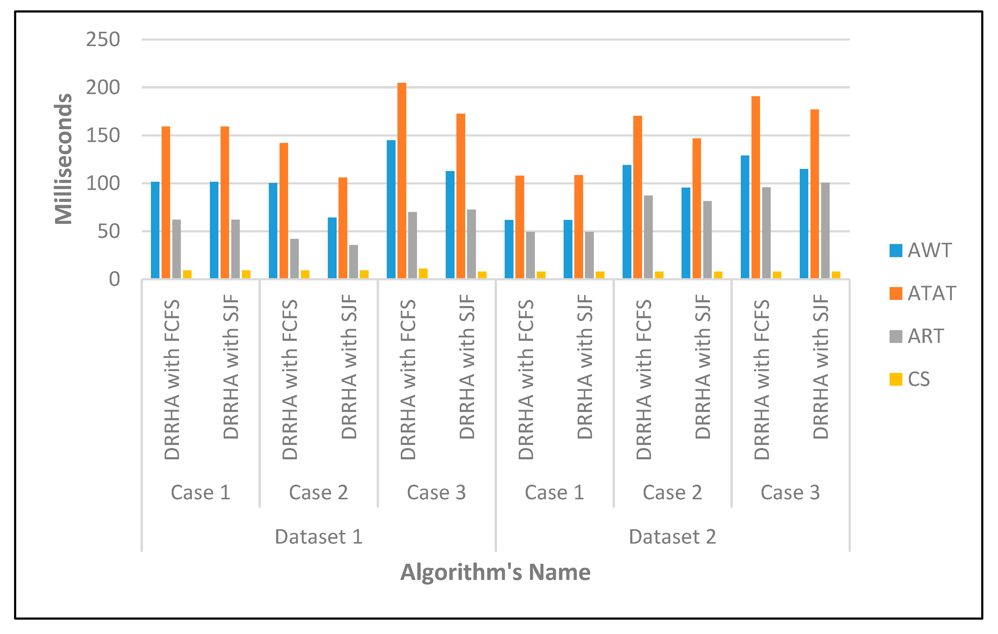
6.1. Evaluation of the Proposed Model (DRRHA) Considering SJF

To evaluate the efficiency of integrating the SJF algorithm with the proposed model, we used the dataset considered in [32]. The dataset consisted of two experiments, where the first one assumed arrival times of zero and the second one took into consideration different arrival times as shown in Table 10. Moreover, each experiment had three cases based on the order of the burst time in increasing order, decreasing order, and a random order.
The evaluations were performed based on the average waiting time, turnaround time, response time, and context switching. Figure 7 presents the evaluation results.
As shown in Figure 7, the integration of the SJF algorithm with the proposed model resulted in a significant reduction in the average waiting time, average turnaround time, and response time in all three cases. It also maintained the number of context switches. Thus, we found that integrating the SJF algorithm with the proposed model had a surprising effect in improving the overall performance, compared with the integration of the FCFS algorithm with the proposed model.

6.2. Comparative Study on the Proposed Model (DRRHA) and the Related Algorithms

The performance of the proposed model was evaluated by conducting several experiments. For fair evaluation, the benchmark was taken from different algorithms and simulated with the same parameters considering the task arrival time and burst time.
We conducted four different evaluations, comparing our proposed algorithm with different related works as follows. (1) The first test was an evaluation to compare our work with the one presented in [16]. (2) The second test was an evaluation to compare our work with the one presented in [33,34]. (3) The third test was an evaluation to compare our work with the one presented in [35]. (4) The fourth test was an evaluation to compare our work with the one presented in [23]. These experiments and evaluation studies are discussed in the following subsections.
A.
The First Test
We conducted two experiments taken from [16], as shown in Table 11, where the proposed model was compared with the traditional RR and IRRVQ algorithms [16] in terms of the average waiting time and average turnaround time.
The proposed model outperformed the other studied algorithms, as shown in Figure 8, which shows clearly that our proposed algorithm decreased both the waiting time and turnaround time for the two cases.
To measure the improvement of the proposed algorithm compared with the one proposed in [16], we calculated the difference between the average waiting times and turnaround time by the following equation, given in [36]:
D i f f e r e n c e = [ | v 1 v 2 | ( v 1 + v 2 ) / 2 ] × 100
where V1 and V2 are the least values.
Table 12 illustrates the improvement of the proposed model over the IRRVQ algorithm [16]. It is clear that the proposed model achieved a 35% improvement in the average waiting time and 23% improvement in the average turnaround time compared with the IRRVQ algorithm [16].
B.
The Second Test
This test included a dataset taken from [33] which consisted of three cases. Table 13 demonstrates these cases in detail. In this experiment, the proposed model was compared with the traditional RR, optimized round-robin [34], and dynamic time slice round-robin algorithms [33]. The comparison was performed based on the average waiting time (AWT), average turnaround time (ATAT), and the number of the context switches (CS).
The results shown in Figure 9 clearly depict that the proposed model demonstrated superior results for the three cases compared with the benchmarked algorithms.
Table 14 shows clearly the high improvement rate of the proposed algorithm compared with the dynamic time slice round-robin algorithm, where our proposed algorithm enhanced the average waiting time by 56%, the average turnaround time by 38%, and the number of context switches by 65%.
C.
The Third Test
In this experiment, the dataset was adopted from [35], which had three different cases as shown in Table 15. In each case, the proposed model was evaluated and compared with the traditional RR algorithm and the benchmarked algorithm in [35]. Moreover, the evaluation process was conducted based on the average waiting time, average turnaround time, and number of context switches.
The obtained results are presented in Figure 10, which shows that our proposed model achieved a significant improvement in performance over the other compared algorithms. For the first case, the performance of the DRRHA in terms of the average waiting time and turnaround time was slightly higher than the improved RR algorithm [35]. On the other hand, regarding the number of context switches, it is noted that the improved RR algorithm [35] recorded 9 CSs, whereas the proposed DRRHA recorded 8 CSs. However, the performance of the proposed DRRHA was still considered acceptable. In contrast, for other evaluated cases, it is noted that the performance of the proposed algorithm achieved remarkably high performance in all the evaluated metrics.
The improvement rate of the proposed algorithm compared with the benchmarks was measured in the third test, and the results have been presented in Table 16. The statistics show that our proposed algorithm achieved an overall 29% improvement in the average waiting time, 20% improvement in the average turnaround time, and finally a 16% improvement in the number of context switches.
D.
The Fourth Test
For this evaluation, the dataset was taken from [23], which was divided into two experiments based on the arrival time of the tasks. Each one, in turn, was divided into two cases as shown in Table 17. The dataset was used to evaluate the proposed model by conducting a comparison with the traditional RR and SRDQ algorithms [23].
Figure 11 shows the superiority of the proposed model compared with the other algorithms for all the comparison criteria. Although the traditional RR algorithm recorded a slight reduction in the average waiting time in the third case compared with the proposed model, the overall results show that the proposed algorithm had a significant reduction in the average waiting time, turnaround time, and number of context switches compared with the traditional RR and SRDQ algorithms.
Table 18 illustrates the improvement rate of the proposed algorithm, where the proposed algorithm obtained a 29% improvement in the average waiting time and 13% improvement in the average turnaround time.

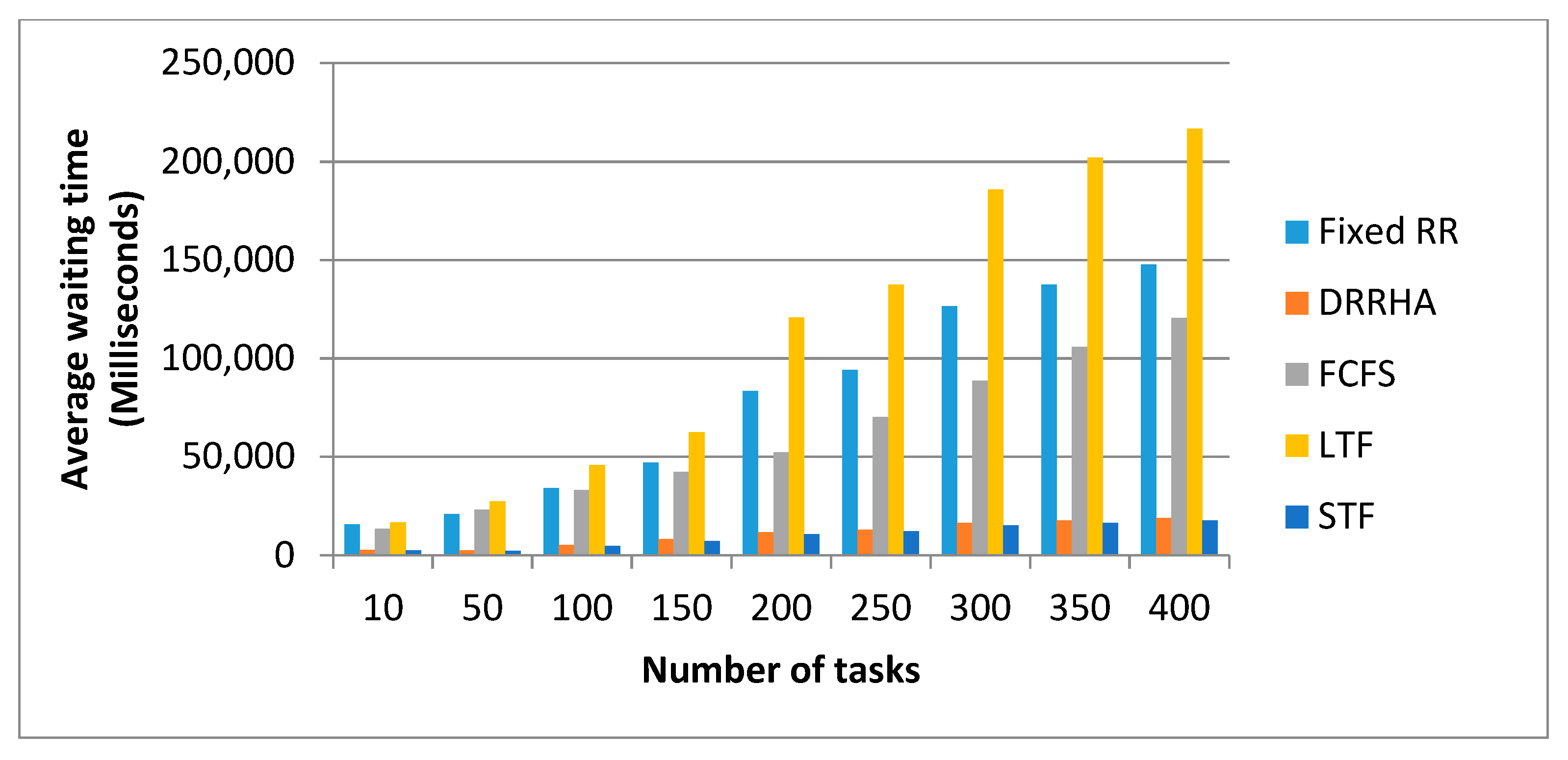
6.3. Evaluating the Performance of the Proposed Model (DRRHA) Using Datasets

In this experiment, the proposed model was validated by conducting several experiments on two different datasets, including the NASA dataset [37,38] and a randomly generated dataset. The performance of the proposed model was measured based on the average waiting time, average turnaround time, and average response time under the same simulation conditions of the previous cases shown in Table 19. The performance of the proposed model was compared to the other conventional algorithms, including FCFS, STF, LTF, and fixed RR. It is worth mentioning that this analytical comparison was performed on one virtual machine, and the experiments were repeated several times while increasing the number of tasks each time to verify the stability of the results.
A.
The First Experiment Using the NASA Dataset
The dataset used for this experiment was the one from NASA [37,38], which has been used in various research such as in [39,40,41]. In this experiment, only the execution time was taken into account. This is because the tasks in the NASA dataset arrived one by one, and therefore there was no overlap in the arrival time of the tasks and, accordingly, these arrival times were not suitable to be used for validating the proposed model. For this reason, the tasks’ arrival times were discarded and replaced by a zero arrival time in the first case and a non-zero arrival time in the second case.
For the first experiment using the NASA dataset with a zero arrival time, the DRRHA was evaluated, assuming that all tasks had the same arrival time. From Figure 12, Figure 13 and Figure 14, we found the following observations:
(1)
The SJF algorithm and the DRRHA achieved the best performance, while the LJF algorithm was the worst;
(2)
There was a clear convergence in the performance of both the SJF algorithm and the DRRHA;
(3)
Although the SJF algorithm succeeded in reducing the average waiting time by 9.31% and the average turnaround time by 8.01%, the DRRHA succeeded in reducing the average response time by 38.38%, as shown in Figure 15, Figure 16 and Figure 17;
(4)
The algorithms maintained the same performance despite the repeated experiments with an increasing number of tasks each time.
For the second case using the NASA dataset with a non-zero arrival time, the DRRHA was evaluated using the NASA dataset assuming the tasks had different arrival times. What could be concluded clearly from these experiments are as follows.
(1)
The superiority of the SJF algorithms and the proposed model in optimizing the performance is shown in Figure 18, Figure 19 and Figure 20;
(2)
Despite the superiority of these two algorithms and the convergence of their performance, it was found that the SJF algorithm outperformed the others in reducing the average waiting time by 12.61% and the turnaround time by 12.29%, while the DRRHA outperformed the others in reducing the average response time by 19.89%;
(3)
On the other hand, the longest job first (LJF) algorithm was the worst among the other algorithms.
B.
The Second Experiment Using a Random Dataset
The dataset used in this experiment was generated randomly within a specific range of the tasks’ burst times and the tasks’ arrival times. This range was defined to be 100–400 for the tasks’ burst times and 10–100 for the tasks’ arrival times. Moreover, this dataset has been commonly used with traditional algorithms like FCFS, shortest task first (STF), LJF, and RR. It should also be noted that when applying the fixed RR algorithm on this random dataset, we considered the following:
(1)
Calculating the optimal time quantum for each experiment using the mean of the burst times;
(2)
Repeating every experiment 50 times and then taking the average values of the waiting time, turnaround time, and response time.
To evaluate our proposed model (DRRHA), the random dataset was used to conduct two different experiments. The first experiment was where the arrival time of the tasks was zero, and the tasks’ burst times were generated randomly. The second experiment randomly generated both the arrival time and the tasks’ burst times. Both experiments were applied to our proposed model and the traditional algorithms mentioned above. Moreover, these experiments were repeated several times while increasing the number of tasks each time to ensure the steadiness of the algorithms’ performances.
For the first case using the random dataset with a zero arrival time, we evaluated the DRRHA using the randomly generated dataset while assuming all tasks arrived at the same time. From Figure 21, Figure 22 and Figure 23, we observed the following:
(1)
The STF algorithm and the DRRHA had the best comparable performances;
(2)
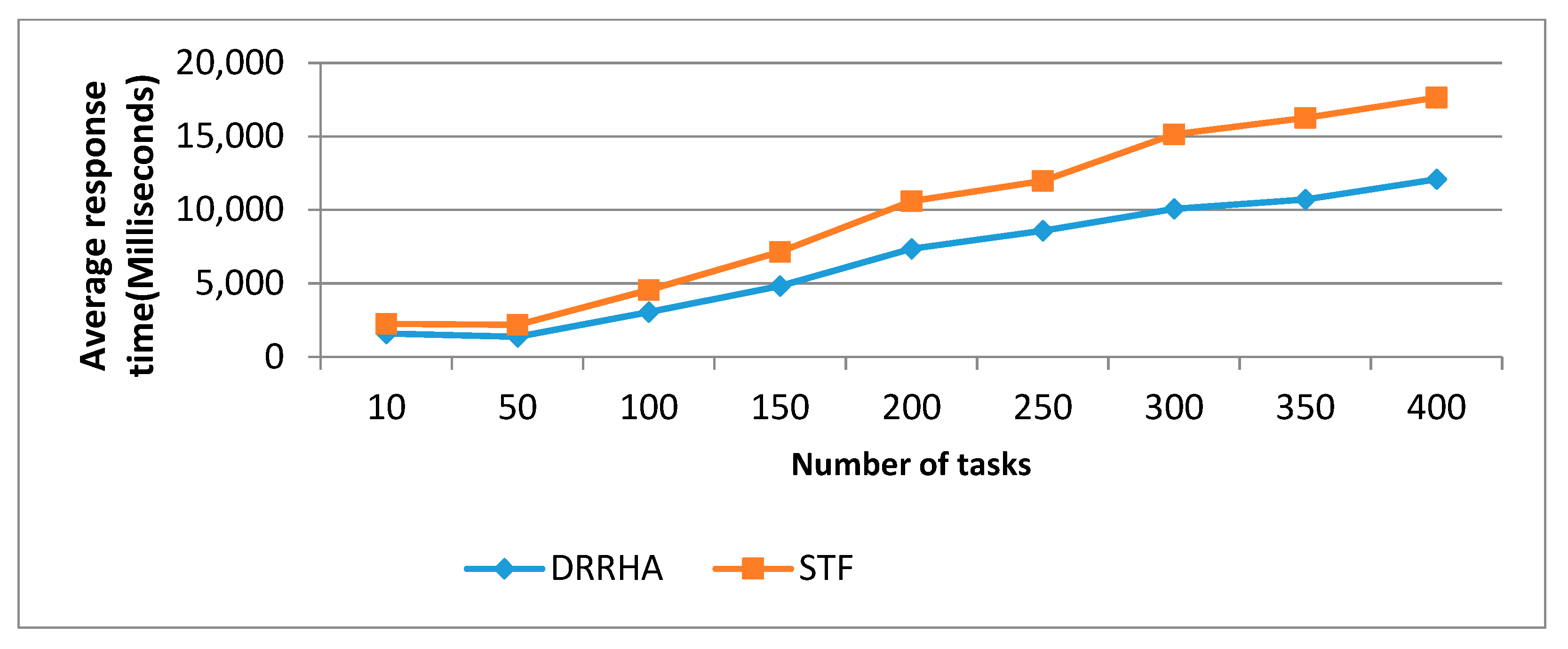
The STF algorithm was slightly superior to the DRRHA in terms of the average waiting time by 21.09% and the turnaround time by 20.31%. However, the DRRHA outperformed the others in terms of decreasing the response time by 35.98%;
(3)
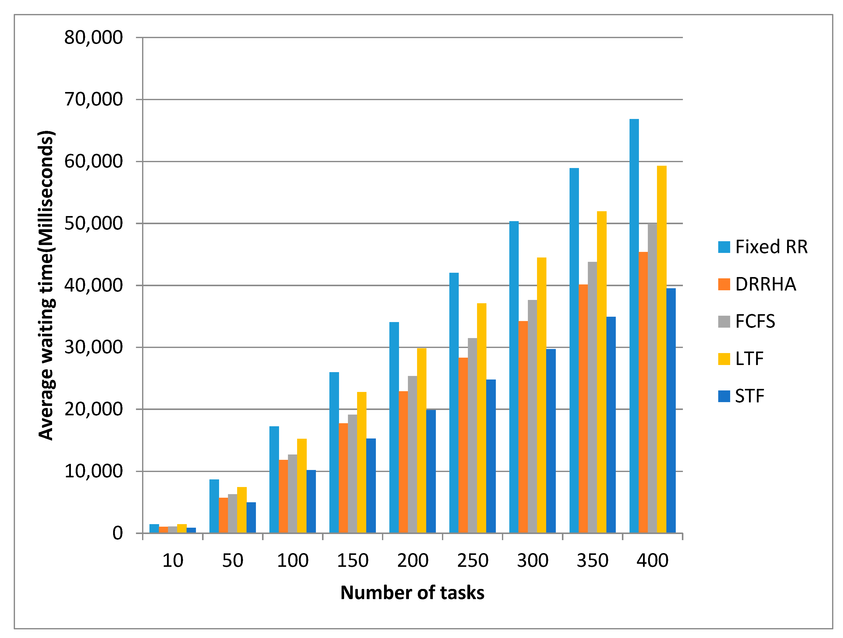
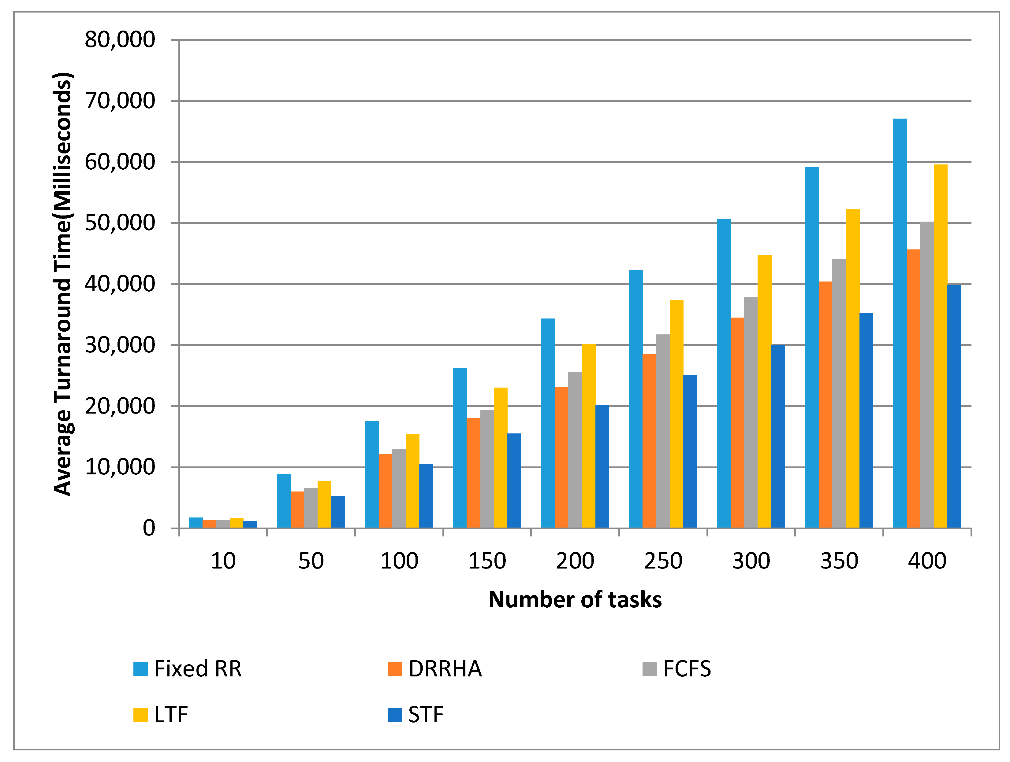
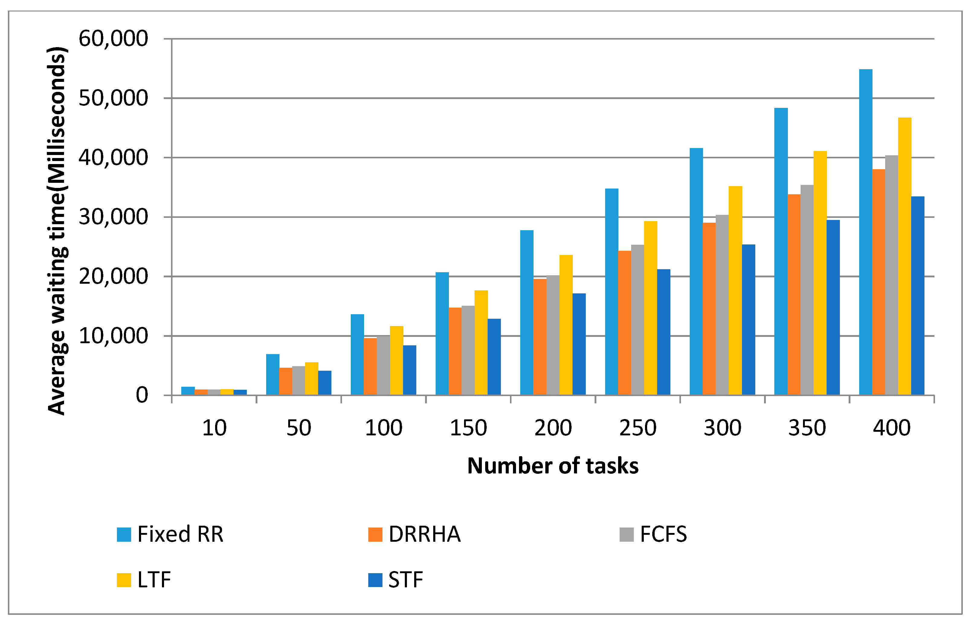
In contrast, the fixed RR algorithm had the worst performance in terms of reducing the average waiting time and turnaround time. The LJF algorithm was the worst in terms of reducing the average response time.
For the second case using the random dataset with a non-zero arrival time, the DRRHA was evaluated using the randomly generated dataset while assuming the tasks arrived at different times. Figure 24, Figure 25 and Figure 26 present the experiments’ results with the following observations:
(1)
The STF algorithm and DRRHA outperformed the other algorithms in optimizing performance;
(2)
Both the STF algorithm and DRRHA had comparable performances, but the STF succeeded in reducing the average waiting time by 18.8% and reducing the average turnaround time by 18.34%. However, the DRRHA reduced the average response time by 29.65%;
(3)
The fixed RR algorithm had the worst performance, as it recorded high values in the average waiting time and turnaround time;
(4)
The LTF algorithm had the worst performance among other algorithms in terms of the average response time.
As a summary, the overall results from the previous experiments indicate the following:
  • For all the cases, the SJF algorithm and the proposed algorithm (DRRHA) achieved the best performance compared with the other algorithms;
  • The SJF algorithm outperformed the DRRHA in terms of the average waiting time and turnaround time. This is because of the SJF algorithm mechanism, which executed the whole task in one round. In contrast, the DRRHA executed the task in several rounds, which may have led to putting the task in the ready queue several times;
  • The DRRHA outperformed the SJF algorithm in terms of the average response time. This is because the DRRHA is preemptive, in which the current task might be paused to give a chance to another task in the ready queue. The SJF algorithm mechanism allows for responding to any new task after completing the entire previous task, which results in increasing the response time;
  • When using the NASA dataset, the LJF algorithm had the worst performance among the other algorithms. This is because of the mechanism of the LJF algorithm, which imposes the implementation of the longest task in the queue first. In addition, the LJF algorithm does not allow for executing the next task until the current one is finished, which results in increasing the waiting time, turnaround time, and response time.
When using the dataset that was generated randomly, the fixed RR algorithm achieved the worst performance in terms of the waiting time and turnaround time. The LJF algorithm achieved the worst performance in terms of the response time. These results of the fixed RR were because of the fixed quantum time, as well as not applying the remaining burst time principle, resulting in increasing the overhead of the algorithm and being inefficient.

7. Conclusions

Task scheduling is one of the critical challenges that affects the overall performance of the cloud computing environment. The major contribution of this paper is enhancing the round-robin algorithm by proposing a novel technique named DRRHA. It concentrates on providing a solution for the time quantum problem by calculating the mean for all the tasks in the ready queue, which is sorted based on the SJF manner. The process of tuning the time quantum dynamically is repeated for each task separately and for each round. Moreover, checking the remaining burst time of the task is an essential principle applied with our proposed algorithm. If the remaining burst time is less than or equal to the current task quantum, the task execution is completed and then removed from the ready queue. Otherwise, the task is stored at the end of the ready queue to be executed in the next round. Various experiments were conducted using the CloudSim Plus tool to evaluate the DRRHA. From the obtained experimental results, it can be concluded that our proposed algorithm (DRRHA) succeeded in optimizing the waiting time, turnaround time, and response time compared with the IRRVQ algorithm, dynamic time slice round-robin algorithm, improved RR algorithm, and SRDQ algorithm.

8. Future Work

This study can be considered a starting point for researchers, as there are still some issues that can be solved and improved in future works, including (1) improving the RR algorithm by finding a new approach for time quantum calculation that combines the dynamic and fixed quantum values to improve the RR algorithm performance, (2) applying new techniques such as fuzzy logic and neural networks to predict the best quantum values of tasks automatically, (3) integrating the RR algorithm with other meta-heuristic algorithms to achieve better performance, and (4) more datasets holding a high number of tasks can be used to evaluate the proposed algorithm, as well as the other related task scheduling algorithms.

Author Contributions

Conceptualization, T.Z.B. and F.A.; investigation, T.Z.B. and F.A.; methodology, T.Z.B. and F.A.; validation, T.Z.B. and F.A.; writing—original draft preparation, T.Z.B.; supervision, F.A.; writing—review and editing, T.Z.B. and F.A. All authors have read and agreed to the published version of the manuscript.

Funding

This research received no external funding.

Institutional Review Board Statement

Not applicable.

Informed Consent Statement

Not applicable.

Data Availability Statement

Not applicable.

Conflicts of Interest

The authors declare no conflict of interest.

References

  1. Razaque, A.; Vennapusa, N.R.; Soni, N.; Janapati, G.S.; Vangala, K.R. Task scheduling in Cloud computing. In Proceedings of the 2016 IEEE Long Island Systems, Applications and Technology Conference (LISAT), Farmingdale, NY, USA, 29 April 2016; Volume 8. [Google Scholar]
  2. Ohlman, B.; Eriksson, A.; Rembarz, R. What networking of information can do for cloud computing. In Proceedings of the Workshop on Enabling Technologies: Infrastructure for Collaborative Enterprises, WETICE, Groningen, The Netherlands, 29 June–1 July 2009; pp. 78–83. [Google Scholar]
  3. Taneja, B. An empirical study of most fit, max-min and priority task scheduling algorithms in cloud computing. In Proceedings of the International Conference on Computing, Communication & Automation, ICCCA 2015, Greater Noida, India, 15–16 May 2015; pp. 664–667. [Google Scholar]
  4. Lynn, T.; Xiong, H.; Dong, D.; Momani, B.; Gravvanis, G.A.; Filelis-Papadopoulos, C.; Elster, A.; Muhammad Zaki Murtaza Khan, M.; Tzovaras, D.; Giannoutakis, K.; et al. CLOUDLIGHTNING: A framework for a self-organising and self-managing heterogeneous cloud. In Proceedings of the CLOSER 2016, 6th International Conference on Cloud Computing and Services Science, Rome, Italy, 23–25 April 2016; Volume 1, pp. 333–338. [Google Scholar]
  5. Giannoutakis, K.M.; Filelis-Papadopoulos, C.K.; Gravvanis, G.A.; Tzovaras, D. Evaluation of self-organizing and self-managing heterogeneous high performance computing clouds through discrete-time simulation. Concurr. Comput. Pract. Exp. 2021, 33, e6326. [Google Scholar]
  6. Soltani, N.; Soleimani, B.; Barekatain, B. Heuristic Algorithms for Task Scheduling in Cloud Computing: A Survey. Int. J. Comput. Netw. Inf. Secur. 2017, 9, 16–22. [Google Scholar] [CrossRef] [Green Version]
  7. Alhaidari, F.; Balharith, T.; Al-Yahyan, E. Comparative analysis for task scheduling algorithms on cloud computing. In Proceedings of the 2019 International Conference on Computer and Information Sciences, ICCIS 2019, Sakaka, Saudi Arabia, 3–4 April 2019; pp. 1–6. [Google Scholar]
  8. Li, X.; Zheng, M.C.; Ren, X.; Liu, X.; Zhang, P.; Lou, C. An improved task scheduling algorithm based on potential games in cloud computing. In Pervasive Computing and the Networked World; Zu, Q., Vargas-Vera, M., Hu, B., Eds.; ICPCA/SWS; Lecture Notes in Computer Science; Springer: Cham, Switzerland, 2013; Volume 8351. [Google Scholar]
  9. Tawfeek, M.; El-Sisi, A.; Keshk, A.; Torkey, F. Cloud task scheduling based on ant colony optimization. Int. Arab J. Inf. Technol. 2015, 12, 129–137. [Google Scholar]
  10. Masdari, M.; Salehi, F.; Jalali, M.; Bidaki, M. A Survey of PSO-Based Scheduling Algorithms in Cloud Computing. J. Netw. Syst. Manag. 2017, 25, 122–158. [Google Scholar] [CrossRef]
  11. Varma, P.S. A finest time quantum for improving shortest remaining burst round robin (srbrr) algorithm. J. Glob. Res. Comput. Sci. 2013, 4, 10–15. [Google Scholar]
  12. Singh, M.; Agrawal, R. Modified Round Robin algorithm (MRR). In Proceedings of the 2017 IEEE International Conference on Power, Control, Signals and Instrumentation Engineering, ICPCSI 2017, Chennai, India, 21–22 September 2017; pp. 2832–2839. [Google Scholar]
  13. Dorgham, O.H.M.; Nassar, M.O. Improved Round Robin Algorithm: Proposed Method to Apply {SJF} using Geometric Mean. Int. J. Adv. Stud. Comput. Sci. Eng. 2016, 5, 112–119. [Google Scholar]
  14. Balharith, T.; Alhaidari, F. Round Robin Scheduling Algorithm in CPU and Cloud Computing: A review. In Proceedings of the 2nd International Conference on Computer Applications and Information Security, ICCAIS 2019, Riyadh, Saudi Arabia, 1–3 May 2019; pp. 1–7. [Google Scholar]
  15. Tayal, S. Tasks scheduling optimization for the cloud computing systems. Int. J. Adv. Eng. Sci. Technol. 2011, 5, 111–115. [Google Scholar]
  16. Mishra, M.K.; Rashid, F. An Improved Round Robin CPU Scheduling Algorithm with Varying Time Quantum. Int. J. Comput. Sci. Eng. Appl. 2014, 4, 1–8. [Google Scholar]
  17. Jbara, Y.H. A new improved round robin-based scheduling algorithm-a comparative analysis. In Proceedings of the 2019 International Conference on Computer and Information Sciences, ICCIS 2019, Sakaka, Saudi Arabia, 3–4 April 2019; pp. 1–6. [Google Scholar]
  18. Srujana, R.; Roopa, Y.M.; Mohan, M.D.S.K. Sorted round robin algorithm. In Proceedings of the International Conference on Trends in Electronics and Informatics, ICOEI 2019, Tirunelveli, India, 23–25 April 2019; pp. 968–971. [Google Scholar]
  19. Sangwan, P.; Sharma, M.; Kumar, A. Improved round robin scheduling in cloud computing. Adv. Comput. Sci. Technol. 2017, 10, 639–644. [Google Scholar]
  20. Fiad, A.; Maaza, Z.M.; Bendoukha, H. Improved Version of Round Robin Scheduling Algorithm Based on Analytic Model. Int. J. Networked Distrib. Comput. 2020, 8, 195. [Google Scholar] [CrossRef]
  21. Faizan, K.; Marikal, A.; Anil, K. A Hybrid Round Robin Scheduling Mechanism for Process Management. Int. J. Comput. Appl. 2020, 177, 14–19. [Google Scholar] [CrossRef]
  22. Biswas, D. Samsuddoha Determining Proficient Time Quantum to Improve the Performance of Round Robin Scheduling Algorithm. Int. J. Mod. Educ. Comput. Sci. 2019, 11, 33–40. [Google Scholar] [CrossRef]
  23. Elmougy, S.; Sarhan, S.; Joundy, M. A novel hybrid of Shortest job first and round Robin with dynamic variable quantum time task scheduling technique. J. Cloud Comput. 2017, 6, 12. [Google Scholar] [CrossRef] [Green Version]
  24. Zhou, J.; Dong, S.B.; Tang, D.Y. Task Scheduling Algorithm in Cloud Computing Based on Invasive Tumor Growth Optimization. Jisuanji Xuebao/Chin. J. Comput. 2018, 41, 1360–1375. [Google Scholar]
  25. Pradhan, P.; Behera, P.K.; Ray, B. Modified Round Robin Algorithm for Resource Allocation in Cloud Computing. Procedia Comput. Sci. 2016, 85, 878–890. [Google Scholar] [CrossRef] [Green Version]
  26. Dave, B.; Yadev, S.; Mathuria, M.; Sharma, Y.M. Optimize task scheduling act by modified round robin scheme with vigorous time quantum. In Proceedings of the International Conference on Intelligent Sustainable Systems, ICISS 2017, Palladam, India, 7–8 December 2017; pp. 905–910. [Google Scholar]
  27. Mishra, M.K. An improved round robin cpu scheduling algorithm. J. Glob. Res. Comput. Sci. 2012, 3, 64–69. [Google Scholar]
  28. Fayyaz, H.A.H.S.; Din, S.M.U.; Iqra. Efficient Dual Nature Round Robin CPU Scheduling Algorithm: A Comparative Analysis. Int. J. Multidiscip. Sci. Eng. 2017, 8, 21–26. [Google Scholar]
  29. Filho, M.C.S.; Oliveira, R.L.; Monteiro, C.C.; Inácio, P.R.M.; Freire, M.M. CloudSim Plus: A cloud computing simulation framework pursuing software engineering principles for improved modularity, extensibility and correctness. In Proceedings of the IM 2017—2017 IFIP/IEEE International Symposium on Integrated Network and Service Management, Lisbon, Portugal, 8–12 May 2017; pp. 400–406. [Google Scholar]
  30. Calheiros, R.N.; Ranjan, R.; Beloglazov, A.; De Rose, C.A.F.; Buyya, R. CloudSim: A toolkit for modeling and simulation of cloud computing environments and evaluation of resource provisioning algorithms. Softw. Pract. Exp. 2010, 41, 23–50. [Google Scholar] [CrossRef]
  31. Saeidi, S.; Baktash, H.A. Determining the Optimum Time Quantum Value in Round Robin Process Scheduling Method. Int. J. Inf. Technol. Comput. Sci. 2012, 4, 67–73. [Google Scholar] [CrossRef] [Green Version]
  32. Nayak, D.; Malla, S.K.; Debadarshini, D. Improved Round Robin Scheduling using Dynamic Time Quantum. Int. J. Comput. Appl. 2012, 38, 34–38. [Google Scholar] [CrossRef]
  33. Muraleedharan, A.; Antony, N.; Nandakumar, R. Dynamic Time Slice Round Robin Scheduling Algorithm with Unknown Burst Time. Indian J. Sci. Technol. 2016, 9, 16. [Google Scholar] [CrossRef] [Green Version]
  34. Hemamalini, M.; Srinath, M.V. Memory Constrained Load Shared Minimum Execution Time Grid Task Scheduling Algorithm in a Heterogeneous Environment. Indian J. Sci. Technol. 2015, 8. [Google Scholar] [CrossRef]
  35. Negi, S. An Improved Round Robin Approach using Dynamic Time Quantum for Improving Average Waiting Time. Int. J. Comput. Appl. 2013, 69, 12–16. [Google Scholar] [CrossRef] [Green Version]
  36. Lang, L.H.P.; Litzenberger, R.H. Dividend announcements. Cash flow signalling vs. free cash flow hypothesis? J. Financ. Econ. 1989, 24, 181–191. [Google Scholar] [CrossRef]
  37. Feitelson, D.G.; Tsafrir, D.; Krakov, D. Experience with using the Parallel Workloads Archive. J. Parallel Distrib. Comput. 2014, 74, 2967–2982. [Google Scholar] [CrossRef] [Green Version]
  38. Nasa-Workload. 2019. Available online: http://www.cs.huji.ac.il/labs/parallel/workload (accessed on 14 August 2019).
  39. Aida, K. Effect of job size characteristics on job scheduling performance. In Job Scheduling Strategies for Parallel Processing; Feitelson, D.G., Rudolph, L., Eds.; Lecture Notes in Computer Science; JSSPP 2000; Springer: Berlin/Heidelberg, Germany, 2000; Volume 1911. [Google Scholar]
  40. Alboaneen, D.A.; Tianfield, H.; Zhang, Y. Glowworm swarm optimisation based task scheduling for cloud computing. In Proceedings of the Second International Conference on Internet of things, Data and Cloud Computing, Cambridge, UK, 22–23 March 2017; pp. 1–7. [Google Scholar]
  41. Chiang, S.H.; Vernon, M.K. Dynamic vs. Static quantum-based parallel processor allocation. In Workshop on Job Scheduling Strategies for Parallel Processing; JSSPP 1996; Lecture Notes in Computer Science; Feitelson, D.G., Rudolph, L., Eds.; Springer: Berlin/Heidelberg, Germany, 1996; Volume 1162. [Google Scholar] [CrossRef]
Figure 1. Comparison of the proposed model integrated with SJF and FCFS.
Computers 10 00063 g001
Figure 2. The proposed model.
Computers 10 00063 g002
Figure 3. The proposed algorithm’s flow chart.
Computers 10 00063 g003
Figure 4. The Gantt chart of round one of the case study.
Computers 10 00063 g004
Figure 5. The Gantt chart of round two of the case study.
Computers 10 00063 g005
Figure 6. The Gantt chart of round three of the case study.
Computers 10 00063 g006
Figure 7. Comparison of the proposed model integrated with SJF and FCFS.
Computers 10 00063 g007
Figure 8. First test’s comparison of results.
Computers 10 00063 g008
Figure 9. Comparison of the results for the second test.
Computers 10 00063 g009
Figure 10. Comparison of results for the third test.
Computers 10 00063 g010
Figure 11. Comparison of results in the fourth test.
Computers 10 00063 g011
Figure 12. The evaluation of the average waiting time with a dataset with a zero arrival time.
Computers 10 00063 g012
Figure 13. The evaluation of the average turnaround time with the NASA dataset with a zero arrival time.
Computers 10 00063 g013
Figure 14. The evaluation of the average response time with a NASA dataset with a zero arrival time.
Computers 10 00063 g014
Figure 15. The performance of the proposed model and SJF algorithm in terms of the average waiting time, with the first experiment having a zero arrival time.
Computers 10 00063 g015
Figure 16. Performance of the proposed model and SJF algorithm in terms of the average turnaround time, with the first experiment having a zero arrival time.
Computers 10 00063 g016
Figure 17. The performance of the proposed model and SJF algorithm in terms of the average response time, with the first experiment having a zero arrival time.
Computers 10 00063 g017
Figure 18. The evaluation of the average waiting time with the NASA dataset with a non-zero arrival time.
Computers 10 00063 g018
Figure 19. The evaluation of the average turnaround time with the NASA dataset with a non-zero arrival time.
Computers 10 00063 g019
Figure 20. The evaluation of the average response time with the NASA dataset with a non-zero arrival time.
Computers 10 00063 g020
Figure 21. The evaluation of the average waiting time with the random dataset with a zero arrival time.
Computers 10 00063 g021
Figure 22. The evaluation of the average turnaround time with the random dataset with a zero arrival time.
Computers 10 00063 g022
Figure 23. The evaluation of the average response time with the random dataset with a zero arrival time.
Computers 10 00063 g023
Figure 24. The evaluation of the average waiting time with the random dataset with a non-zero arrival time.
Computers 10 00063 g024
Figure 25. The evaluation of the average turnaround time with the random dataset with a non-zero arrival time.
Computers 10 00063 g025
Figure 26. The evaluation of the average response time with the random dataset with a non-zero arrival time.
Computers 10 00063 g026
Table 1. Dataset used in the analytical study.
Datasets with Zero Arrival Time
TaskCase 1
Increasing Order
Case 2
Decreasing Order
Case 3
Random Order
Arrival TimeBurst TimeArrival TimeBurst TimeArrival TimeBurst Time
T102001050105
T2025085060
T30350550120
T4050043048
T5080035075
T6090----
Table 2. Case study.
TaskArrival TimeBurst Time
T1012
T208
T3123
T4210
T5330
T6415
Table 3. Round one of the case study.
Round 1M = 10M/2 = 5
TasksQTij = (M/2) + (M/2)/BTijRemaining BTij
T25.6252.375
T15.4166.584
Table 4. Round 2 of the case study after applying SJF.
TaskBurst Time
T16.584
T410
T615
T323
T530
Table 5. Round two of the case study.
Round 2M = 16.91M/2 = 8.45
TasksQTij = (M/2) + (M/2)/BTijRemaining BTij
T19.730
T49.290.71
T69.015.99
T38.8114.19
T58.7321.27
Table 6. Case study of the RQ in round two.
TaskBurst Time
T314.19
T521.27
Table 7. Round three of the case study.
Round 3M = 17.73M/2 = 8.86
TasksQTij = (M/2) + (M/2)/BTijRemaining BTij
T39.484.71
T59.2712
Table 8. The evaluation results of the case study.
TaskArrival TimeBurst TimeWTTATRT
T10128200
T208085.416
T312352.7375.7313.416
T4210182822.22
T5330659532.22
T6415264140.95
Average28.2883344.6216719.037
Table 9. Configuration table for simulation.
Data Center Characteristics
ParametersValues
Data Center OSLinux
Data Center VMMXen
Data Center ArchitectureX86
VM Parameters
Image Size10,000
VM_MIPS1000
Bandwidth50,000
VM Number of CPUs10
Ram512
Cloudlet Parameters
Cloudlet File Size300
Cloudlet Output Size300
Cloudlet Utilization (CPU, BW, Ram)Full
Table 10. Data sets with zero arrival time.
Data Sets with Zero Arrival TimeData Sets with Non-Zero Arrival Time
TaskCase 1
Increasing Order
Case 2
Decreasing Order
Case 3
Random Order
Case 1
Increasing Order
Case 2
DecreasingOrder
Case 3
Random Order
Arrival TimeBurst TimeArrival TimeBurst TimeArrival TimeBurst TimeArrival TimeBurst TimeArrival TimeBurst TimeArrival TimeBurst Time
T1030077080014080065
T2034054045234274172
T3062045062645370450
T4074019034862418643
T50880140781477514780
Table 11. First test with a random dataset with zero and non-zero arrival times.
CASE 1CASE 2
TaskArrival TimeBurst TimeTaskArrival TimeBurst Time
T1015070
T20324254
T301010510
T4026153615
T5020171817
Table 12. The improvement rate in the first test.
First Test
The MetricsCase 1Case 2
Improvement (%)Improvement (%)
Avg. WT35%12%
Avg. TAT23%6%
Table 13. Second test with a dataset with zero and non-zero arrival times.
TaskCase 1Case 2Case 3
Arrival TimeBurst TimeArrival TimeBurst TimeArrival TimeBurst Time
T1014033015
T2034222477
T30455481530
T40627702085
T5077974--
Table 14. The improvement rate in the second test.
Second Test
The MetricsCase 1Case 2Case 3Overall
Improvement (%)Improvement (%)Improvement (%)Improvement (%)
Avg.
WT
58%54%56%56%
Avg.
TAT
38%39%38%38%
CS61%61%74%65%
Table 15. Third test’s dataset.
TaskCase 1Case 2Case 3
Arrival TimeBurst TimeArrival TimeBurst TimeArrival TimeBurst Time
T1012042011
T2011032010
T3022082022
T4031045031
T5021022025
T6----013
Table 16. Improvement rate in the third test.
Third Test
The MetricsCase 1Case 2Case 3Overall
Improvement (%)Improvement (%)Improvement (%)Improvement (%)
Avg. WT6%53%28%29%
Avg. TAT4%35%20%20%
CS−12%50%10%16%
Table 17. Dataset with zero and non-zero arrival times in the fourth test.
Zero Arrival TimeNon-Zero Arrival Time
TaskCase 1Case 2Case 3Case 4
Arrival TimeBurst TimeArrival TimeBurst TimeArrival TimeBurst TimeArrival TimeBurst Time
T1020010018010
T2040014470614
T30600708741370
T40800120168021120
Table 18. The improvement rate in the fourth test.
Fourth Test
The MetricsCase 1Case 2Case 3Case 4Overall
Improvement (%)Improvement (%)Improvement (%)Improvement (%)Improvement (%)
Avg. WT10%9%34%63%29%
Avg. TAT6%4%19%24%13%
Table 19. The improvement rate in all cases.
MetricsThe Improvement Rate Achieved by the Proposed Model Compared with the Following Algorithms
IRRVQDTSRRImproved RR [35]SRDQ
Avg. WT12%56%29%29%
Avg. TAT6%38%20%13%
No.CS12%65%16%
Publisher’s Note: MDPI stays neutral with regard to jurisdictional claims in published maps and institutional affiliations.

