


FabNet: A Features Agglomeration-Based Convolutional Neural Network for Multiscale Breast Cancer Histopathology Images Classification
Abstract
:Simple Summary
Abstract
1. Introduction
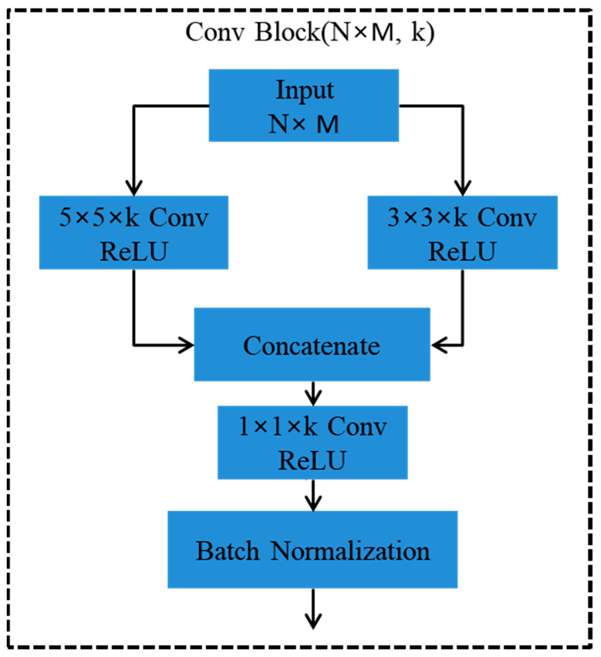
- We proposed a FabNet model that can learn the fine-to-coarse structural and textural features of multi-scale histopathological images by accretive network architecture that agglomerate hierarchical feature maps to acquire significant classification accuracy.
- To preserve and integrate the features, our model links convolutional blocks in a closely coupled tree-based architecture. This method employs every layer of the network from the shallowest to the deepest layers to learn about the rich patterns that occupy a large portion of the feature pile.
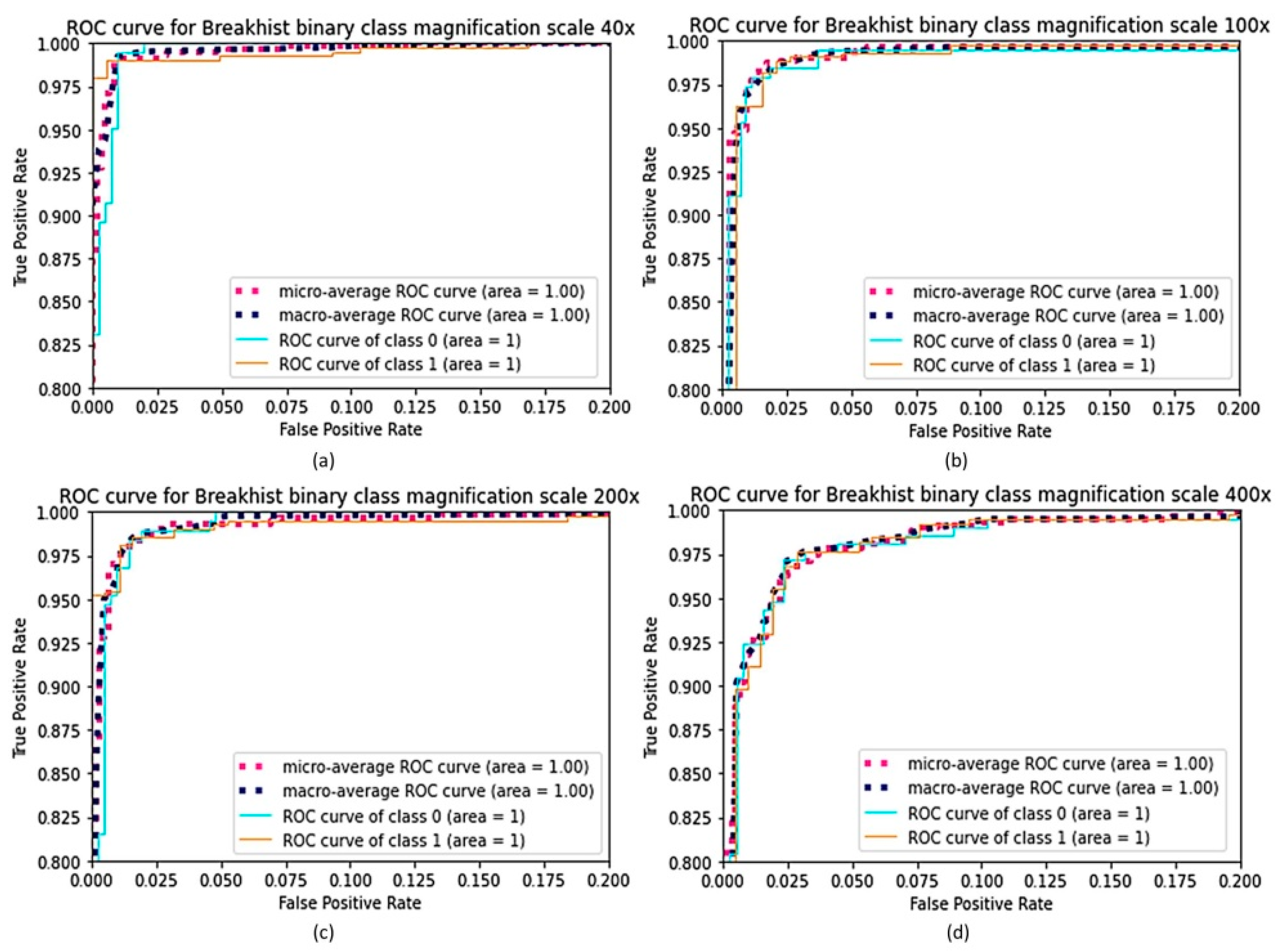
- We assessed the FabNet model using two publicly available standard datasets that are related to breast cancer and colorectal cancer and noticed that it outperforms the current state-of-the-art models in terms of accuracy, F1 score, sensitivity, and precision when we evaluated our model at different magnification scales of both binary and multi classification.
2. Related Works
2.1. Conventional Learning Methods
2.2. Deep Learning Approaches
3. FabNet: Features Agglomeration Approach
4. Methodology
4.1. Dataset
4.1.1. BreaHis
4.1.2. NCT-CRC-HE-100K
4.2. Image Representation and Patch Extraction
5. Experimental Results
5.1. Model Training
5.2. Implementation Details
6. Conclusions
Author Contributions
Funding
Institutional Review Board Statement
Informed Consent Statement
Data Availability Statement
Conflicts of Interest
References
- Rahhal, M.M.A. Breast Cancer Classification in Histopathological Images Using Convolutional Neural Network. Int. J. Adv. Comput. Sci. Appl. IJACSA 2018, 9. [Google Scholar] [CrossRef]
- Alom, M.Z.; Yakopcic, C.; Nasrin, M.S.; Taha, T.M.; Asari, V.K. Breast Cancer Classification from Histopathological Images with Inception Recurrent Residual Convolutional Neural Network. J. Digit. Imaging 2019, 32, 605–617. [Google Scholar] [CrossRef]
- Araújo, T.; Aresta, G.; Castro, E.; Rouco, J.; Aguiar, P.; Eloy, C.; Polónia, A.; Campilho, A. Classification of Breast Cancer Histology Images Using Convolutional Neural Networks. PloS ONE 2017, 12, e0177544. [Google Scholar] [CrossRef] [PubMed]
- Liu, Y.; Chen, C.; Wang, X.; Sun, Y.; Zhang, J.; Chen, J.; Shi, Y. An Epigenetic Role of Mitochondria in Cancer. Cells 2022, 11, 2518. [Google Scholar] [CrossRef] [PubMed]
- Chen, K.; Zhang, J.; Beeraka, N.M.; Tang, C.; Babayeva, Y.V.; Sinelnikov, M.Y.; Zhang, X.; Zhang, J.; Liu, J.; Reshetov, I.V.; et al. Advances in the Prevention and Treatment of Obesity-Driven Effects in Breast Cancers. Front. Oncol. 2022, 12, 2663. [Google Scholar] [CrossRef]
- Chen, K.; Lu, P.; Beeraka, N.M.; Sukocheva, O.A.; Madhunapantula, S.V.; Liu, J.; Sinelnikov, M.Y.; Nikolenko, V.N.; Bulygin, K.V.; Mikhaleva, L.M.; et al. Mitochondrial Mutations and Mitoepigenetics: Focus on Regulation of Oxidative Stress-Induced Responses in Breast Cancers. Semin. Cancer Biol. 2022, 83, 556–569. [Google Scholar] [CrossRef] [PubMed]
- Xie, P.; Ma, Y.; Yu, S.; An, R.; He, J.; Zhang, H. Development of an Immune-Related Prognostic Signature in Breast Cancer. Front. Genet. 2020, 10, 1390. [Google Scholar] [CrossRef]
- Williamson, G.R.; Plowright, H.; Kane, A.; Bunce, J.; Clarke, D.; Jamison, C. Collaborative Learning in Practice: A Systematic Review and Narrative Synthesis of the Research Evidence in Nurse Education. Nurse Educ. Pract. 2020, 43, 102706. [Google Scholar] [CrossRef]
- Bardou, D.; Zhang, K.; Ahmad, S.M. Classification of Breast Cancer Based on Histology Images Using Convolutional Neural Networks. IEEE Access 2018, 6, 24680–24693. Available online: https://www.google.com/search?q=Bardou%2C+D.%3B+Zhang%2C+K.%3B+Ahmad%2C+S.M.+Classification+of+Breast+Cancer+Based+on+Histology+Images+Using+Convolutional+Neural+Networks.+Ieee+Access+2018%2C+6%2C+24680%E2%80%9324693.&rlz=1C1ONGR_enPK996PK996&oq=Bardou%2C+D.%3B+Zhang%2C+K.%3B+Ahmad%2C+S.M.+Classification+of+Breast+Cancer+Based+on+Histology+Images+Using+Convolutional+Neural+Networks.+Ieee+Access+2018%2C+6%2C+24680%E2%80%9324693.&aqs=chrome..69i57.1132j0j4&sourceid=chrome&ie=UTF-8 (accessed on 31 August 2022). [CrossRef]
- Mccann, M.T.; Ozolek, J.A.; Castro, C.A.; Parvin, B.; Kovacevic, J.; Mccann, M.T.; Member, S.; Ozolek, J.A.; Castro, C.A.; Parvin, B.; et al. Automated Histology Analysis: Opportunities for Signal Processing. IEEE Signal Process. Mag. 2014, 32, 78–87. [Google Scholar] [CrossRef]
- Robertson, S.; Azizpour, H.; Smith, K.; Hartman, J. Digital Image Analysis in Breast Pathology—From Image Processing Techniques to Artificial Intelligence. Transl. Res. 2018, 194, 19–35. [Google Scholar] [CrossRef] [PubMed]
- Ching, T.; Himmelstein, D.S.; Beaulieu-Jones, B.K.; Kalinin, A.A.; Do, B.T.; Way, G.P.; Ferrero, E.; Agapow, P.-M.; Zietz, M.; Hoffman, M.M.; et al. Opportunities and Obstacles for Deep Learning in Biology and Medicine. J. R. Soc. Interface 2018, 15, 20170387. [Google Scholar] [CrossRef] [PubMed]
- Iglovikov, V.; Shvets, A. TernausNet: U-Net with VGG11 Encoder Pre-Trained on ImageNet for Image Segmentation. arXiv 2018, arXiv:1801.05746. [Google Scholar]
- Raman, R.; Srinivasan, S.; Virmani, S.; Sivaprasad, S.; Rao, C.; Rajalakshmi, R. Fundus Photograph-Based Deep Learning Algorithms in Detecting Diabetic Retinopathy. Eye 2019, 33, 97–109. [Google Scholar] [CrossRef]
- Tiulpin, A.; Thevenot, J.; Rahtu, E.; Lehenkari, P.; Saarakkala, S. Automatic Knee Osteoarthritis Diagnosis from Plain Radiographs: A Deep Learning-Based Approach. Sci. Rep. 2018, 8, 1727. [Google Scholar] [CrossRef] [PubMed]
- Ma, X.; Niu, Y.; Gu, L.; Wang, Y.; Zhao, Y.; Bailey, J.; Lu, F. Understanding Adversarial Attacks on Deep Learning Based Medical Image Analysis Systems. Pattern Recognit. 2021, 110, 107332. [Google Scholar] [CrossRef]
- Sanyal, R.; Jethanandani, M.; Sarkar, R. DAN: Breast Cancer Classification from High-Resolution Histology Images Using Deep Attention Network. In Innovations in Computational Intelligence and Computer Vision; Sharma, M.K., Dhaka, V.S., Perumal, T., Dey, N., Tavares, J.M.R.S., Eds.; Springer: Singapore, 2021; pp. 319–326. [Google Scholar]
- Kumar, S.; Sharma, S. Sub-Classification of Invasive and Non-Invasive Cancer from Magnification Independent Histopathological Images Using Hybrid Neural Networks. Evol. Intell. 2022, 15, 1531–1543. [Google Scholar] [CrossRef]
- Dou, J. Clinical Decision System Using Machine Learning and Deep Learning: A Survey. 2022. Available online: https://www.researchgate.net/profile/Jason-Dou/publication/360154101_Clinical_Decision_System_using_Machine_Learning_and_Deep_Learning_a_Survey/links/630b86f5acd814437fe29fe7/Clinical-Decision-System-using-Machine-Learning-and-Deep-Learning-a-Survey.pdf (accessed on 31 August 2022).
- Amin, M.S.; Ahn, H. Earthquake Disaster Avoidance Learning System Using Deep Learning. Cogn. Syst. Res. 2021, 66, 221–235. [Google Scholar] [CrossRef]
- Amin, M.S.; Yasir, S.M.; Ahn, H. Recognition of Pashto Handwritten Characters Based on Deep Learning. Sensors 2020, 20, E5884. [Google Scholar] [CrossRef]
- Sadiq, A.M.; Ahn, H.; Choi, Y.B. Human Sentiment and Activity Recognition in Disaster Situations Using Social Media Images Based on Deep Learning. Sensors 2020, 20, 7115. [Google Scholar] [CrossRef]
- Lin, M.; Chen, Q.; Yan, S. Network in Network. 2014. Available online: https://arxiv.org/abs/1312.4400 (accessed on 31 August 2022).
- Szegedy, C.; Liu, W.; Jia, Y.; Sermanet, P.; Reed, S.; Anguelov, D.; Erhan, D.; Vanhoucke, V.; Rabinovich, A. Going Deeper with Convolutions 2014. arXiv 2014, arXiv:1409.4842. [Google Scholar]
- He, K.; Zhang, X.; Ren, S.; Sun, J. Identity Mappings in Deep Residual Networks. In Proceedings of the Computer Vision–ECCV 2016: 14th European Conference, Amsterdam, The Netherlands, 11–14 October 2016; Springer International Publishing: Berlin/Heidelberg, Germany, 2016. [Google Scholar]
- Srivastava, R.K.; Greff, K.; Schmidhuber, J. Highway Networks. arXiv 2015, arXiv:1505.00387. [Google Scholar]
- Yasrab, R. SRNET: A Shallow Skip Connection Based Convolutional Neural Network Design for Resolving Singularities. J. Comput. Sci. Technol. 2019, 34, 924–938. [Google Scholar] [CrossRef]
- Vapnik, V.N. The Nature of Statistical Learning Theory; Springer: New York, NY, USA, 2000; ISBN 978-1-4419-3160-3. [Google Scholar]
- Kowal, M.; Filipczuk, P.; Obuchowicz, A.; Korbicz, J.; Monczak, R. Computer-Aided Diagnosis of Breast Cancer Based on Fine Needle Biopsy Microscopic Images. Comput. Biol. Med. 2013, 43, 1563–1572. [Google Scholar] [CrossRef] [PubMed]
- Spanhol, F.A.; Oliveira, L.S.; Petitjean, C.; Heutte, L. A Dataset for Breast Cancer Histopathological Image Classification. IEEE Trans. Biomed. Eng. 2016, 63, 1455–1462. [Google Scholar] [CrossRef] [PubMed]
- George, Y.M.; Zayed, H.H.; Roushdy, M.I.; Elbagoury, B.M. Remote Computer-Aided Breast Cancer Detection and Diagnosis System Based on Cytological Images. IEEE Syst. J. 2014, 8, 949–964. [Google Scholar] [CrossRef]
- Breast Cancer Diagnosis from Biopsy Images with Highly Reliable Random Subspace Classifier Ensembles |SpringerLink. Available online: https://link.springer.com/article/10.1007/s00138-012-0459-8 (accessed on 31 August 2022).
- Robinson, E.; Silverman, B.G.; Keinan-Boker, L. Using Israel’s National Cancer Registry Database to Track Progress in the War against Cancer: A Challenge for Health Services. Isr. Med. Assoc. J. IMAJ 2017, 19, 221–224. [Google Scholar]
- Gupta, V.; Bhavsar, A. Breast Cancer Histopathological Image Classification: Is Magnification Important? In Proceedings of the 2017 IEEE Conference on Computer Vision and Pattern Recognition Workshops (CVPRW), Honolulu, HI, USA, 21–26 July 2017; pp. 769–776. [Google Scholar]
- Seo, H.; Brand, L.; Barco, L.S.; Wang, H. Scaling Multi-Instance Support Vector Machine to Breast Cancer Detection on the BreaKHis Dataset. Bioinformatics 2022, 38, i92–i100. [Google Scholar] [CrossRef]
- Rashmi, R.; Prasad, K.; Udupa, C.B.K. Breast Histopathological Image Analysis Using Image Processing Techniques for Diagnostic Purposes: A Methodological Review. J. Med. Syst. 2021, 46, 7. [Google Scholar] [CrossRef]
- Gupta, S.; Sinha, N.; Sudha, R.; Babu, C. Breast Cancer Detection Using Image Processing Techniques. In Proceedings of the 2019 Innovations in Power and Advanced Computing Technologies (i-PACT), Piscataway, NJ, USA, 22–23 March 2019; Volume 1, pp. 1–6. [Google Scholar]
- Das, A.; Nair, M.S.; Peter, S.D. Computer-Aided Histopathological Image Analysis Techniques for Automated Nuclear Atypia Scoring of Breast Cancer: A Review. J. Digit. Imaging 2020, 33, 1091–1121. [Google Scholar] [CrossRef] [PubMed]
- Spanhol, F.A.; Oliveira, L.S.; Petitjean, C.; Heutte, L. Breast Cancer Histopathological Image Classification Using Convolutional Neural Networks. In Proceedings of the 2016 International Joint Conference on Neural Networks (IJCNN), Vancouver, BC, Canada, 24–29 July 2016; pp. 2560–2567. [Google Scholar]
- Krizhevsky, A.; Sutskever, I.; Hinton, G.E. ImageNet Classification with Deep Convolutional Neural Networks. In Advances in Neural Information Processing Systems; Curran Associates, Inc.: Red Hook, NY, USA, 2012; Volume 25. [Google Scholar]
- Hou, L.; Samaras, D.; Kurc, T.M.; Gao, Y.; Davis, J.E.; Saltz, J.H. Patch-Based Convolutional Neural Network for Whole Slide Tissue Image Classification. In Proceedings of the 2016 IEEE Conference on Computer Vision and Pattern Recognition (CVPR), Las Vegas, NV, USA, 27–30 June 2016. [Google Scholar]
- Han, Z.; Wei, B.; Zheng, Y.; Yin, Y.; Li, K.; Li, S. Breast Cancer Multi-Classification from Histopathological Images with Structured Deep Learning Model. Sci. Rep. 2017, 7, 4172. [Google Scholar] [CrossRef]
- Cireşan, D.C.; Giusti, A.; Gambardella, L.M.; Schmidhuber, J. Mitosis Detection in Breast Cancer Histology Images with Deep Neural Networks. In Medical Image Computing and Computer-Assisted Intervention—MICCAI 2013; Mori, K., Sakuma, I., Sato, Y., Barillot, C., Navab, N., Eds.; Springer: Berlin, Heidelberg, 2013; pp. 411–418. [Google Scholar]
- Wang, H.; Roa, A.C.; Basavanhally, A.N.; Gilmore, H.L.; Shih, N.; Feldman, M.; Tomaszewski, J.; Gonzalez, F.; Madabhushi, A. Mitosis Detection in Breast Cancer Pathology Images by Combining Handcrafted and Convolutional Neural Network Features. J. Med. Imaging 2014, 1, 034003. [Google Scholar] [CrossRef] [PubMed]
- Kashif, M.N.; Raza, S.E.A.; Sirinukunwattana, K.; Arif, M.; Rajpoot, N. Handcrafted Features with Convolutional Neural Networks for Detection of Tumor Cells in Histology Images. In Proceedings of the 2016 IEEE 13th International Symposium on Biomedical Imaging (ISBI), Prague, Czech Republic, 13–16 April 2016; pp. 1029–1032. [Google Scholar]
- Tellez, D.; Litjens, G.; Bándi, P.; Bulten, W.; Bokhorst, J.-M.; Ciompi, F.; van der Laak, J. Quantifying the Effects of Data Augmentation and Stain Color Normalization in Convolutional Neural Networks for Computational Pathology. Med. Image Anal. 2019, 58, 101544. [Google Scholar] [CrossRef]
- Bejnordi, B.E.; Zuidhof, G.; Balkenhol, M.; Hermsen, M.; Bult, P.; van Ginneken, B.; Karssemeijer, N.; Litjens, G.; Laak, J. van der Context-Aware Stacked Convolutional Neural Networks for Classification of Breast Carcinomas in Whole-Slide Histopathology Images. J. Med. Imaging 2017, 4, 044504. [Google Scholar] [CrossRef] [PubMed]
- Ehteshami Bejnordi, B.; Mullooly, M.; Pfeiffer, R.M.; Fan, S.; Vacek, P.M.; Weaver, D.L.; Herschorn, S.; Brinton, L.A.; van Ginneken, B.; Karssemeijer, N.; et al. Using Deep Convolutional Neural Networks to Identify and Classify Tumor-Associated Stroma in Diagnostic Breast Biopsies. Mod. Pathol. 2018, 31, 1502–1512. [Google Scholar] [CrossRef]
- Reinhard, E.; Ashikhmin, M.; Gooch, B.; Shirley, P. Color Transfer between Images. IEEE Comput. Graph. Appl. 2001, 21, 34–41. [Google Scholar] [CrossRef]
- Vahadane, A.; Peng, T.; Sethi, A.; Albarqouni, S.; Wang, L.; Baust, M.; Steiger, K.; Schlitter, A.M.; Esposito, I.; Navab, N. Structure-Preserving Color Normalization and Sparse Stain Separation for Histological Images. IEEE Trans. Med. Imaging 2016, 35, 1962–1971. [Google Scholar] [CrossRef] [PubMed]
- Mathews, A.; Simi, I.; Kizhakkethottam, J.J. Efficient Diagnosis of Cancer from Histopathological Images By Eliminating Batch Effects. Procedia Technol. 2016, 24, 1415–1422. [Google Scholar] [CrossRef]
- Kather, J.N.; Halama, N.; Marx, A. 100,000 Histological Images of Human Colorectal Cancer and Healthy Tissue 2018. Available online: https://zenodo.org/record/1214456#.Y98AhK1BxPY (accessed on 30 January 2023).
- Macenko, M.; Niethammer, M.; Marron, J.S.; Borland, D.; Woosley, J.T.; Guan, X.; Schmitt, C.; Thomas, N.E. A Method for Normalizing Histology Slides for Quantitative Analysis. In Proceedings of the 2009 IEEE International Symposium on Biomedical Imaging: From Nano to Macro, Boston, MA, USA, 28 June–1 July 2009; IEEE: Boston, MA, USA, 2009; pp. 1107–1110. [Google Scholar]
- Ono, Y.; Trulls, E.; Fua, P.; Yi, K.M. LF-Net: Learning Local Features from Images. Adv. Neural Inf. Process. Syst. 2018, 31. [Google Scholar]
- Man, R.; Yang, P.; Xu, B. Classification of Breast Cancer Histopathological Images Using Discriminative Patches Screened by Generative Adversarial Networks. IEEE Access 2020, 8, 155362–155377. [Google Scholar] [CrossRef]
- Simonyan, K.; Zisserman, A. Very Deep Convolutional Networks for Large-Scale Image Recognition. arXiv 2014, arXiv:1409.1556. [Google Scholar]
- He, K.; Zhang, X.; Ren, S.; Sun, J. Deep Residual Learning for Image Recognition. In Proceedings of the IEEE Conference on Computer Vision and Pattern Recognition, Boston, MA, USA, 7–12 June 2015. [Google Scholar]
- Sheikh, T.S.; Lee, Y.; Cho, M. Histopathological Classification of Breast Cancer Images Using a Multi-Scale Input and Multi-Feature Network. Cancers 2020, 12, 2031. [Google Scholar] [CrossRef] [PubMed]
- Spanhol, F.A.; Oliveira, L.S.; Cavalin, P.R.; Petitjean, C.; Heutte, L. Deep Features for Breast Cancer Histopathological Image Classification. In Proceedings of the 2017 IEEE International Conference on Systems, Man, and Cybernetics (SMC), Banff, AB, Canada, 5–8 October 2017; pp. 1868–1873. [Google Scholar]
- Kumar, K.; Rao, A.C.S. Breast Cancer Classification of Image Using Convolutional Neural Network. In Proceedings of the 2018 4th International Conference on Recent Advances in Information Technology (RAIT), Dhanbad, India, 15–17 March 2018; pp. 1–6. [Google Scholar]
- Sudharshan, P.J.; Petitjean, C.; Spanhol, F.; Oliveira, L.E.; Heutte, L.; Honeine, P. Multiple Instance Learning for Histopathological Breast Cancer Image Classification. Expert Syst. Appl. 2019, 117, 103–111. [Google Scholar] [CrossRef]
- Gour, M.; Jain, S.; Sunil Kumar, T. Residual Learning Based CNN for Breast Cancer Histopathological Image Classification. Int. J. Imaging Syst. Technol. 2020, 30, 621–635. [Google Scholar] [CrossRef]
- Gandomkar, Z.; Brennan, P.C.; Mello-Thoms, C. Computer-Assisted Nuclear Atypia Scoring of Breast Cancer: A Preliminary Study. J. Digit. Imaging 2019, 32, 702–712. [Google Scholar] [CrossRef]
- Wang, C.; Shi, J.; Zhang, Q.; Ying, S. Histopathological Image Classification with Bilinear Convolutional Neural Networks. In Proceedings of the 2017 39th Annual International Conference of the IEEE Engineering in Medicine and Biology Society (EMBC), Jeju Island, Republic of Korea, 11–15 July 2017; pp. 4050–4053. [Google Scholar]
- Sari, C.T.; Gunduz-Demir, C. Unsupervised Feature Extraction via Deep Learning for Histopathological Classification of Colon Tissue Images. IEEE Trans. Med. Imaging 2018, 38, 1139–1149. [Google Scholar] [CrossRef] [Green Version]
- Kather, J.N.; Krisam, J.; Charoentong, P.; Luedde, T.; Herpel, E.; Weis, C.-A.; Gaiser, T.; Marx, A.; Valous, N.A.; Ferber, D.; et al. Predicting Survival from Colorectal Cancer Histology Slides Using Deep Learning: A Retrospective Multicenter Study. PLoS Med. 2019, 16, e1002730. [Google Scholar] [CrossRef]
- Ghosh, S.; Bandyopadhyay, A.; Sahay, S.; Ghosh, R.; Kundu, I.; Santosh, K.C. Colorectal Histology Tumor Detection Using Ensemble Deep Neural Network. Eng. Appl. Artif. Intell. 2021, 100, 104202. [Google Scholar] [CrossRef]
- Mewada, H.K.; Patel, A.V.; Hassaballah, M.; Alkinani, M.H.; Mahant, K. Spectral–Spatial Features Integrated Convolution Neural Network for Breast Cancer Classification. Sensors 2020, 20, 4747. [Google Scholar] [CrossRef] [PubMed]


| Reference | Local/Global | Cancer Type | Staining | Method | Dataset |
|---|---|---|---|---|---|
| Ceresin et al. (2013) [43] | Local-level | Breast | Hematoxylin and eosin | CNN | ICPR2012 (50 images) |
| Wang et al. (2014) [44] | Local-level | Breast | Hematoxylin and eosin | Rippled integration of CNN | ICPR2012 (50 images) |
| Raza et al. (2016) [45] | Local-level | Colorectal | Hematoxylin and eosin | Cell detection Spatially constrained CNN + handcrafted features | Private CRC dataset (15 images) |
| Tellez et al. (2019) [46] | Local-level | Breast | Hematoxylin and eosin; PHH3 | CNN | TNBC (36 images); TUPAC (814 images) |
| Ehteshami et al. (2017) [47] | Global-level | Breast | Hematoxylin and eosin | Stacked CNN incorporating contextual information | Private set (221 images) |
| Ehteshami et al. (2018) [48] | Global-level | Breast | Hematoxylin and eosin | Integration of DHACNN & LSTM | BreakHis (7909 images) |
| Category | Subtypes | Magnification | Sum | Individuals | |||
|---|---|---|---|---|---|---|---|
| 40× | 100× | 200× | 400× | ||||
| Benign | Phyllodes Tumor (PHT) | 149 | 150 | 140 | 130 | 569 | 7 |
| Fibroadenoma (FID) | 253 | 260 | 264 | 237 | 1014 | 10 | |
| Adenosis (ADE) | 114 | 113 | 111 | 106 | 444 | 4 | |
| Tubular Adenona (TUA) | 109 | 121 | 108 | 115 | 453 | 3 | |
| Malignant | Papillary Carcinoma (PAC) | 145 | 142 | 135 | 138 | 560 | 6 |
| Ductal Carcinoma (DUC) | 864 | 903 | 896 | 788 | 3451 | 38 | |
| Lobular Carcinoma (LOC) | 156 | 170 | 163 | 137 | 626 | 5 | |
| Mucinous Carcinoma (MUC) | 205 | 222 | 196 | 169 | 792 | 9 | |
| Dataset | Parameters | FabNet | DenseNet121 | VGG16 | ResNet50 |
|---|---|---|---|---|---|
| BreakHis | Epochs | 100 | 100 | 100 | 100 |
| Learning Rate | |||||
| Batch Size | 16 | 16 | 16 | 16 | |
| Number of layers | 30 | 121 | 16 | 50 | |
| Optimizer | Adam | Adam | Adam | Adam | |
| Number of parameters | 3239 K | 7138 K | 14,765 K | 23,788 K | |
| NCT-CRC-HE-100K | Epochs | 100 | 100 | 100 | 100 |
| Learning Rate | |||||
| Batch Size | 64 | 64 | 64 | 64 | |
| Number of layers | 30 | 121 | 16 | 50 | |
| Optimizer | Adam | Adam | Adam | Adam | |
| Number of parameters | 3239 K | 7138 K | 14,765 K | 23,788 K |
| Accuracy (%) | Method | Magnification Level | |||
|---|---|---|---|---|---|
| 40× | 100× | 200× | 400× | ||
| Patient Level | DenseNet 121 [55] | 92.02 | 90.21 | 81.94 | 80.09 |
| MSI-MFNet [58] | 93.04 | 88.34 | 92.12 | 89.19 | |
| Proposed FabNet | 99.01 | 89.26 | 98.38 | 96.96 | |
| Image Level | DenseNet 121 [55] | 94.26 | 92.71 | 83.90 | 82.75 |
| MSI-MFNet [58] | 94.12 | 89.25 | 92.45 | 90.27 | |
| Proposed FabNet | 99.03 | 89.68 | 98.51 | 97.10 | |
| Class | Model | Accuracy | Sensitivity | |||||||
|---|---|---|---|---|---|---|---|---|---|---|
| Benign | Malignant | |||||||||
| Binary | DenseNet [55] | 0.92 | 0.75 | 0.97 | ||||||
| MSIMFNet [58] | 0.92 | 0.76 | 0.98 | |||||||
| FabNet | 0.99 | 0.989 | 0.990 | |||||||
| ADE | FIB | PHT | TAD | DUC | LOC | MUC | PAC | |||
| Multi | DenseNet121 [55] | 0.84 | 0.60 | 0.84 | 0.72 | 0.84 | 0.86 | 0.85 | 0.97 | 0.91 |
| MSIMFNet [58] | 0.88 | 0.60 | 0.87 | 0.79 | 0.89 | 0.96 | 0.75 | 0.98 | 0.92 | |
| FabNet | 0.97 | 1.00 | 0.88 | 1.00 | 1.00 | 0.804 | 0.89 | 0.784 | 0.865 | |
| Class | Magnification Level | Accuracy (%) | Precision (%) | Recall (%) | F1 Score (%) |
|---|---|---|---|---|---|
| Binary | 40× | 99.00 | 98.991 | 98.986 | 98.989 |
| 100× | 89.26 | 89.128 | 89.262 | 89.195 | |
| 200× | 99.00 | 98.352 | 98.355 | 98.354 | |
| 400× | 97.96 | 97.541 | 97.521 | 97.551 | |
| Multi | 40× | 91.26 | 90.635 | 89.126 | 88.289 |
| 100× | 97.00 | 96.531 | 96.427 | 95.912 | |
| 200× | 97.05 | 85.972 | 85.526 | 85.748 | |
| 400× | 97.20 | 89.947 | 89.851 | 88.899 |
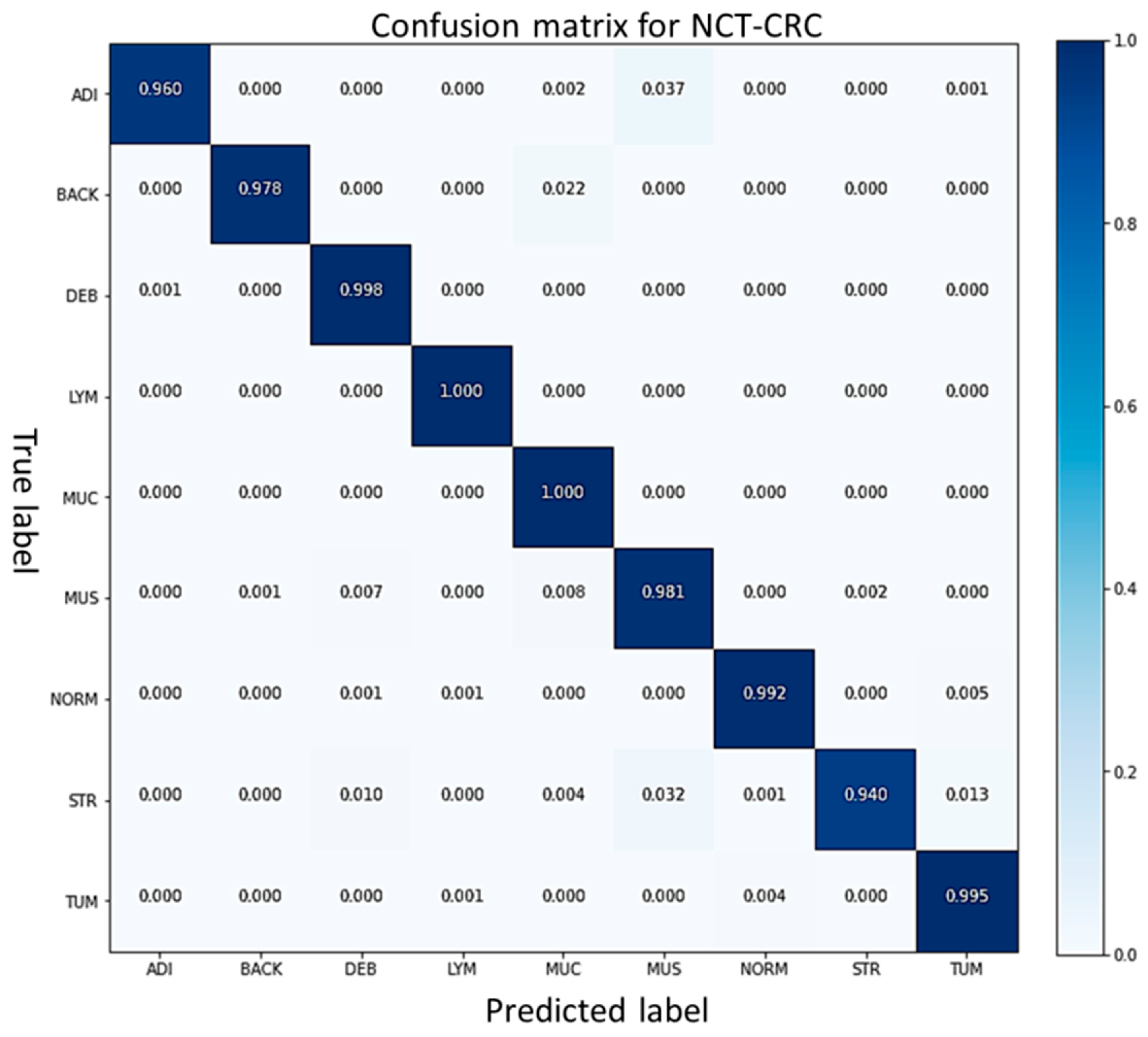
| Model | Accuracy (%) | Sensitivity | ||||||||
|---|---|---|---|---|---|---|---|---|---|---|
| ADI | BACK | DEB | LYM | MUC | MUS | NORM | STR | TUM | ||
| VGG16 [56] | 96.0 | 0.95 | 0.93 | 0.94 | 0.88 | 0.96 | 0.89 | 0.98 | 0.91 | 0.90 |
| ResNet50 [56] | 95.9 | 0.94 | 0.90 | 1.00 | 0.89 | 0.92 | 0.88 | 0.89 | 0.95 | 0.98 |
| Dense Net 121 [55] | 96.1 | 0.96 | 0.70 | 0.98 | 0.97 | 0.92 | 0.91 | 0.96 | 0.93 | 0.94 |
| FabNet | 98.2 | 0.96 | 0.98 | 1.00 | 1.00 | 1.00 | 0.98 | 0.99 | 0.94 | 0.99 |
| Class | Precision | F1 Score | Recall |
|---|---|---|---|
| Adipose Tissue | 1.00 | 0.98 | 0.96 |
| Background | 1.00 | 0.99 | 0.98 |
| Colorectal Cancer | 0.98 | 0.99 | 1.00 |
| Debris | 1.00 | 1.00 | 1.00 |
| Lymphocytes | 0.95 | 0.97 | 1.00 |
| Mucus | 0.94 | 0.96 | 0.98 |
| NC Tumor | 0.99 | 0.99 | 0.99 |
| Colon Mucosa | 1.00 | 0.97 | 0.94 |
| Cancer Stroma | 0.99 | 0.99 | 0.99 |
| Dataset | Author | Year | Preprocessing | Model | Accuracy (%) Magnification Level | |||
|---|---|---|---|---|---|---|---|---|
| 40× | 100× | 200× | 400× | |||||
| Break his Dataset | Spanhol et al. [30] | 2016 | None | PFTAS QDA | 83 ± 4.1 | 82.1 ± 4.9 | 85.1 ± 3.1 | 82 ± 3.8 |
| Spanhol et al. [39] | 2016 | Image Resize | Pre-Trained AlexNet | 88 ± 5.6 | 84.5 ± 2.4 | 85.3 ± 3.8 | 81 ± 4.9 | |
| Spanhol et al. [59] | 2017 | None | DeCAF Model | 84 ± 6.9 | 83.9 ± 5.9 | 86.3 ± 3.5 | 82 ± 2.4 | |
| Kumar et al. [60] | 2018 | Image Resize | Newly Designed CNN | 83 ± 3.2 | 81.0 ± 4.2 | 84.2 ± 3.4 | 81 ± 1.3 | |
| Sudharshan et al. [61] | 2019 | None | PLTAS NPMIL | 92 ± 5.9 | 89.1 ± 5.2 | 87.2 ± 4.3 | 82 ± 3.0 | |
| Gour et al. [62] | 2020 | Data augmentation | ResHist Model | 82 ± 3.3 | 88.1 ± 2.7 | 92.5 ± 2.8 | 87 ± 2.4 | |
| Lingqiao Li et.al [42] | 2018 | Data Augmentation, Transfer learning | NDCNN | 92.8 ± 2.1 | 93.9 ± 1.9 | 93.7 ± 2.2 | 92.9 ± 1.8 | |
| Gandomkar et.al [63] | Data Augmentation, | ResNET152 | 94.18 ± 2.1 | 93.2 ± 1.4 | 94.7 ± 3.6 | 93.5 ± 2.9 | ||
| Proposed | 2021 | Stain Normalization | FabNet | 99 ± 0.2 | 89.51 ± 1.7 | 97.41 ± 1.4 | 96 ± 1.0 | |
| Dataset | Author | Year | Preprocessing | Model | Evaluation Matrices | |||
|---|---|---|---|---|---|---|---|---|
| Colon (NCT-CRC-HE-100K) dataset | Accuracy | Precision | F1 Score | Sensitivity | ||||
| Wang et al. [64] | 2017 | None | BCNN | 92.6 | 91.2 | 92.8 | 90.5 | |
| Sari et al. [65] | 2018 | None | SSAE/SCAE | 93.6 | 93.4 | 93.2 | 92.3 | |
| Kather et al. [66] | 2019 | Stain Normalization | TL+CNN (VGG) | 94.3 | 92.1 | 93.5 | 94.1 | |
| Gosh et al. [67] | 2021 | None | Ensemble DNN | 92.8 | 92.6 | 92.2 | 93.1 | |
| Proposed | 2021 | None | FabNet | 98.3 | 98.3 | 98.2 | 98.2 | |
Disclaimer/Publisher’s Note: The statements, opinions and data contained in all publications are solely those of the individual author(s) and contributor(s) and not of MDPI and/or the editor(s). MDPI and/or the editor(s) disclaim responsibility for any injury to people or property resulting from any ideas, methods, instructions or products referred to in the content. |
© 2023 by the authors. Licensee MDPI, Basel, Switzerland. This article is an open access article distributed under the terms and conditions of the Creative Commons Attribution (CC BY) license (https://creativecommons.org/licenses/by/4.0/).
Share and Cite
Amin, M.S.; Ahn, H. FabNet: A Features Agglomeration-Based Convolutional Neural Network for Multiscale Breast Cancer Histopathology Images Classification. Cancers 2023, 15, 1013. https://doi.org/10.3390/cancers15041013
Amin MS, Ahn H. FabNet: A Features Agglomeration-Based Convolutional Neural Network for Multiscale Breast Cancer Histopathology Images Classification. Cancers. 2023; 15(4):1013. https://doi.org/10.3390/cancers15041013
Chicago/Turabian StyleAmin, Muhammad Sadiq, and Hyunsik Ahn. 2023. "FabNet: A Features Agglomeration-Based Convolutional Neural Network for Multiscale Breast Cancer Histopathology Images Classification" Cancers 15, no. 4: 1013. https://doi.org/10.3390/cancers15041013