
Development of Symbolic Expressions Ensemble for Breast Cancer Type Classification Using Genetic Programming Symbolic Classifier and Decision Tree Classifier


Abstract
:Simple Summary
Abstract
1. Introduction
- Is it possible to apply dataset balancing methods to equalize the number of samples per class and in the end improve the classification accuracy of obtaining SEs?
- Is it possible to use GPSC with the random hyperparameter value selection (RHVS) method, and train using 5-fold cross validation (5CV) to obtain a set of SEs with high classification accuracy for each dataset class?
- Is it possible to combine obtained SEs to create a robust system with high classification accuracy?
- Is it possible to combine the SEs with the decision tree classifier to achieve high classification accuracy?
2. Materials and Methods
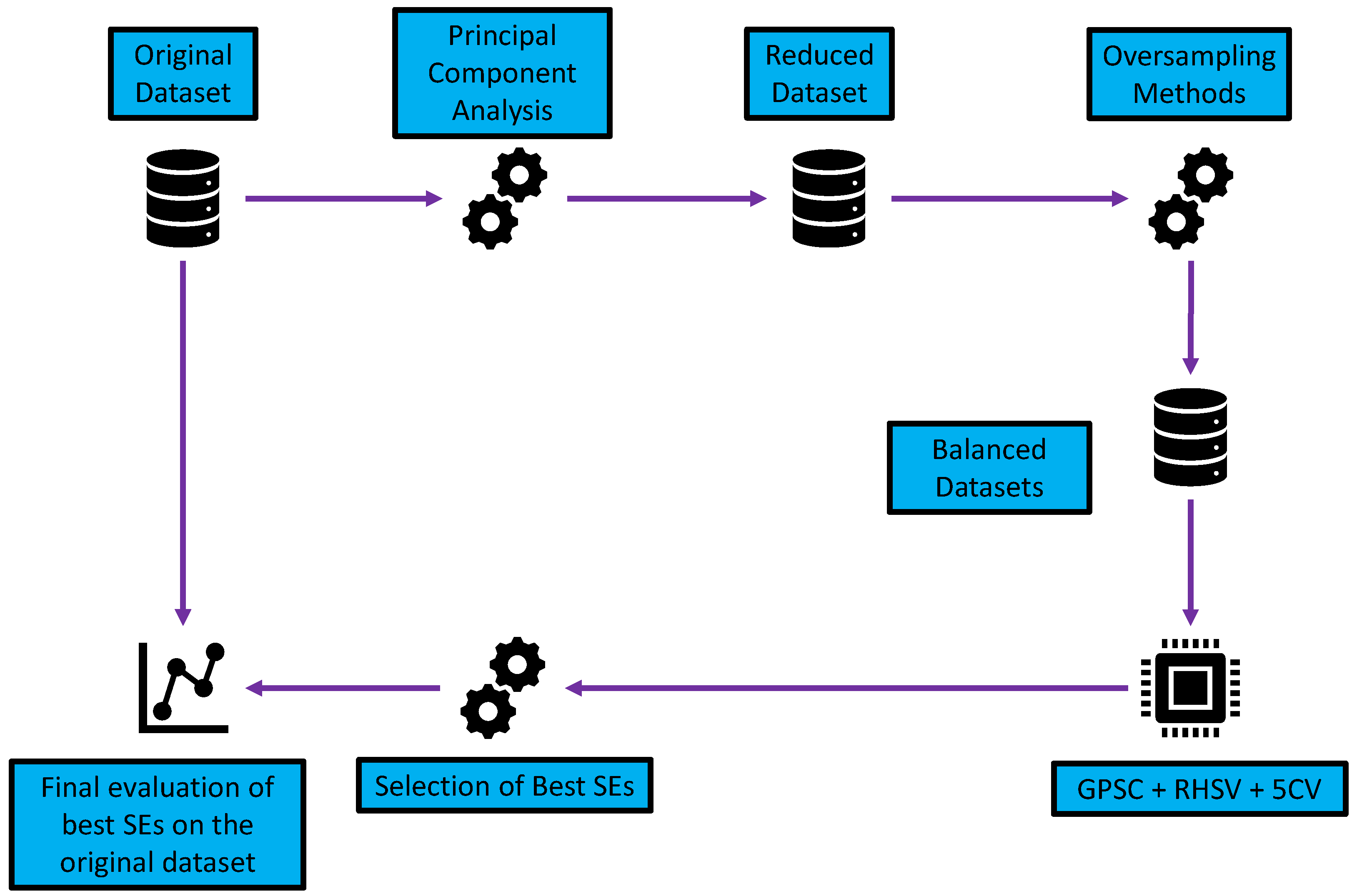
2.1. Research Methodology
- Dimensionality reduction using PCA—reduction in the number of input variables.
- Application of different oversampling methods—the creation of datasets with an equal number of class samples.
- Application of GPSC with RHVS and training using 5CV—using each dataset in GPSC and trained using 5CV to obtain the set of SEs for each class; the RHVS method is used to find the optimal combination of hyperparameters with which the GPSC will generate SEs with high classification accuracy.
- Customized set of SEs—evaluation of the best SEs and creating a robust set of SEs.
- Final evaluation—application of customized set of SEs and SEs + DTC and evaluation on the original dataset.
2.2. Dataset Description
- Large number of input variables (54,676 genes);
- Small number of dataset samples (151 samples);
- Large imbalance between class samples.
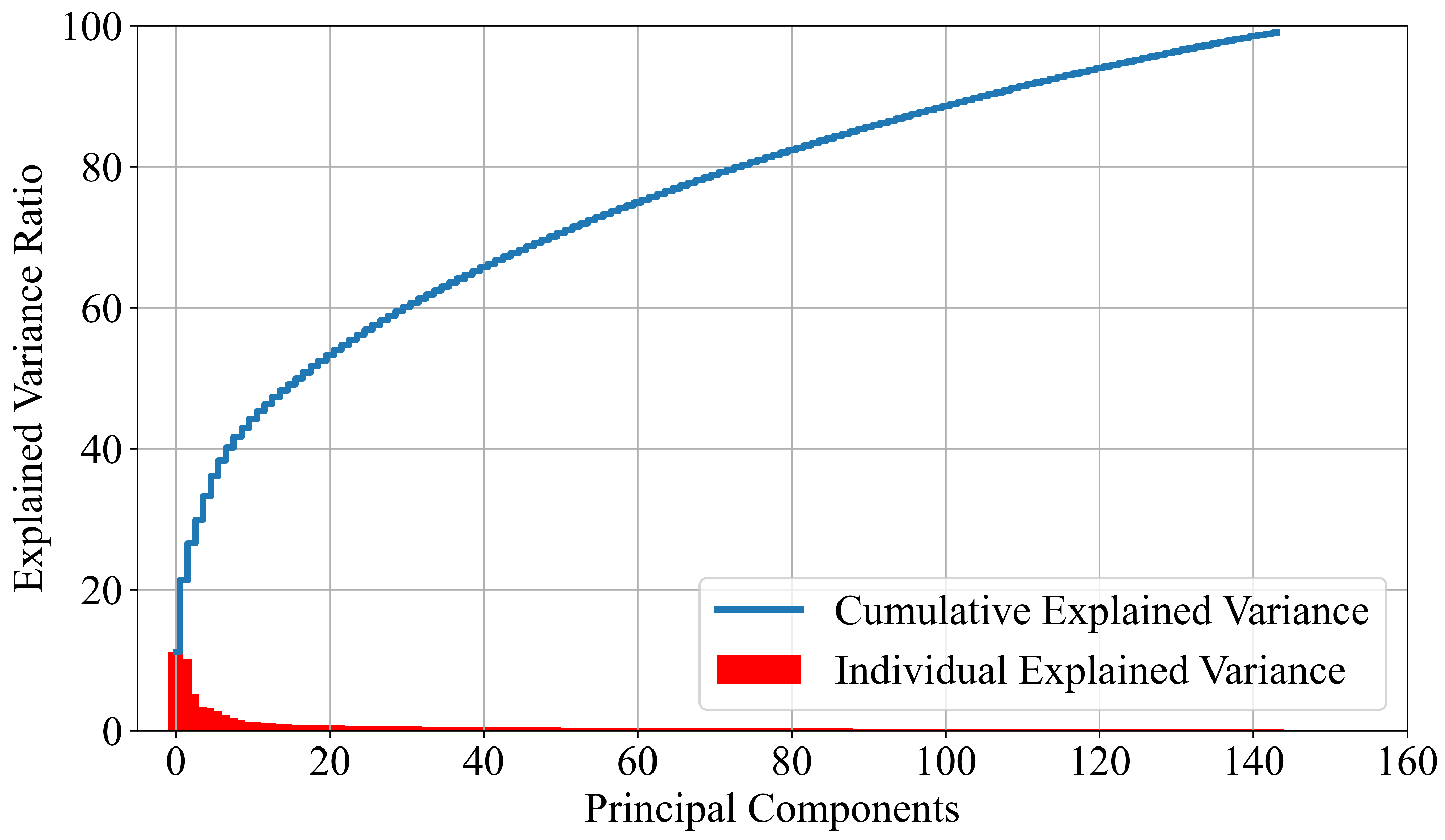
2.2.1. PCA
2.2.2. Target Variable Description and Transformation into Numerical Form
2.3. Oversampling Methods
2.3.1. BorderlineSMOTE
2.3.2. SMOTE
2.3.3. SVM SMOTE
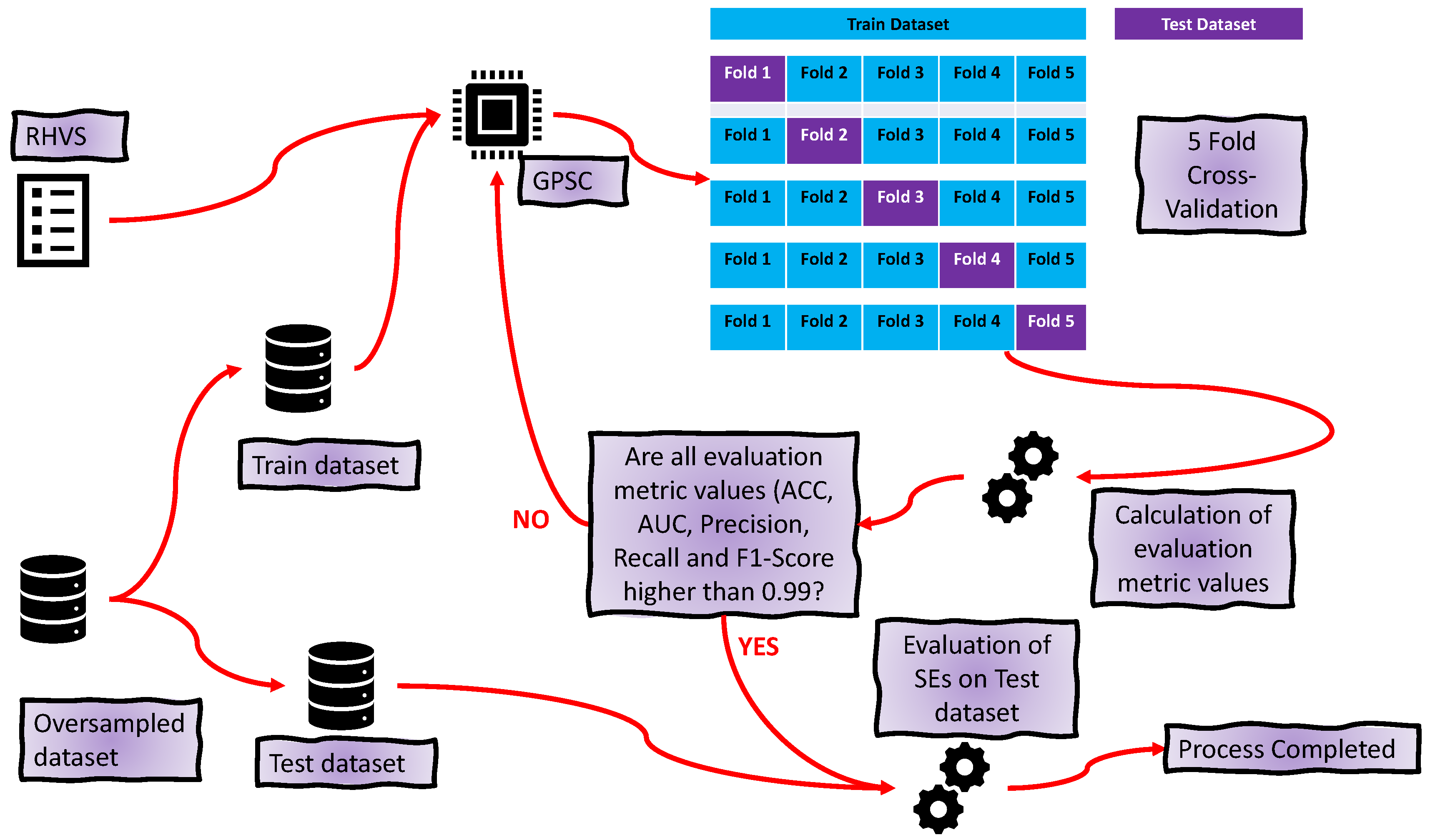
2.4. GPSC with RHVS
- The output of each population member has to be computed by providing values of input variables;
- The previous output is used in the sigmoid function to compute the output. The sigmoid function can be written in the following form:where x is the output obtained from the population member.
- After the sigmoid output is computed, then the LogLoss function is used as the evaluation metric. The LogLoss function can be written aswhere y and p are true value and prediction probability, respectively.

| Hyperparameter Name | Range |
|---|---|
| SizePop | 1000–2000 |
| DepthInit | 3–18 |
| GenNum | 200–300 |
| RangeConst | −10,000–10,000 |
| SizeTour | 100–500 |
| CritStop | – |
| CrossValue | 0.001–0.3 |
| HoistMute | 0.001–0.3 |
| SubMute | 0.9–1.0 |
| PointMute | 0.001–0.3 |
| ParsCoef | – |
2.5. Decision Tree Classifier
2.6. Training Procedure
3. Results
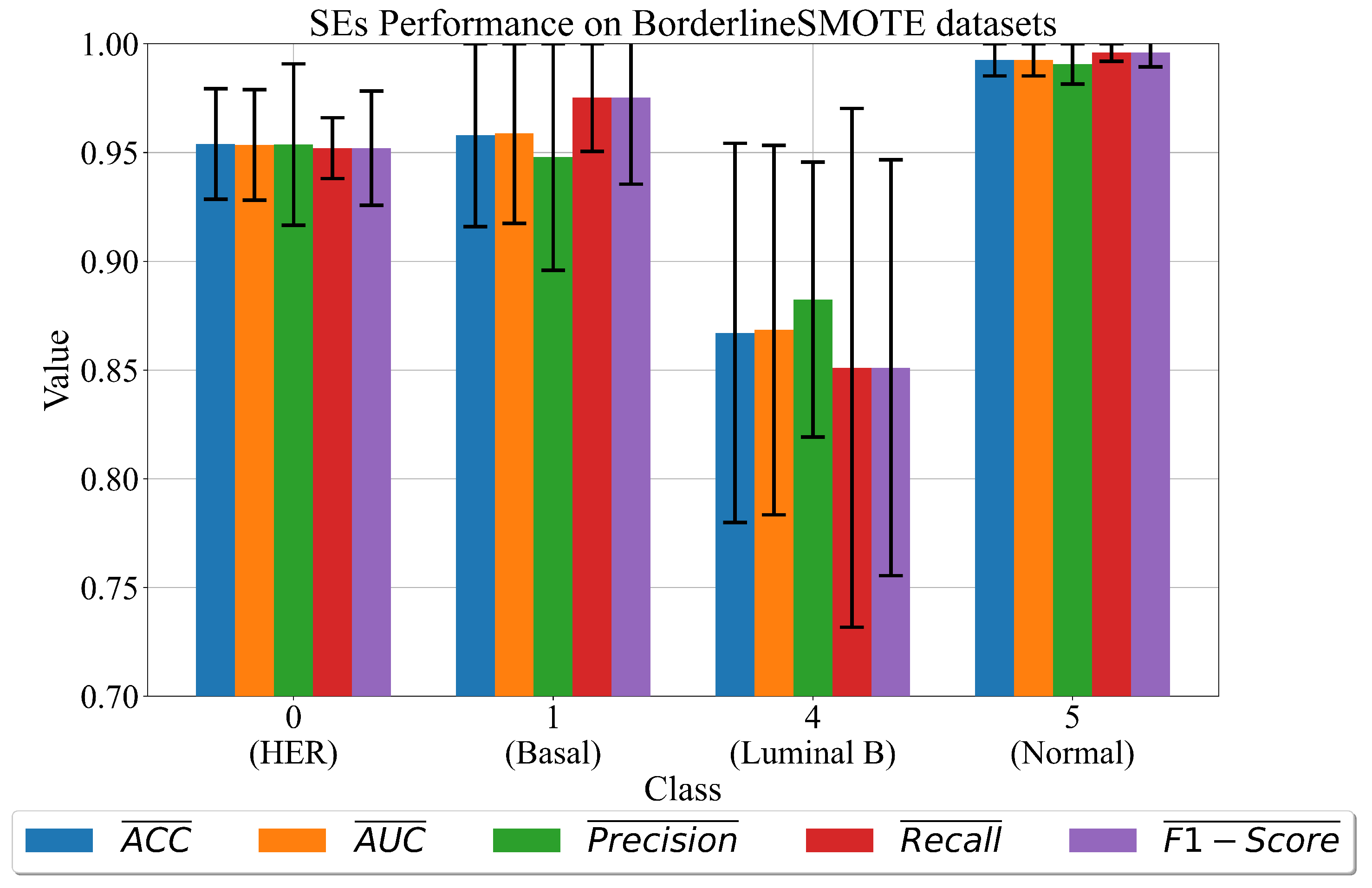
3.1. The Best Set of SEs Obtained on Dataset Balanced with BorderlineSMOTE
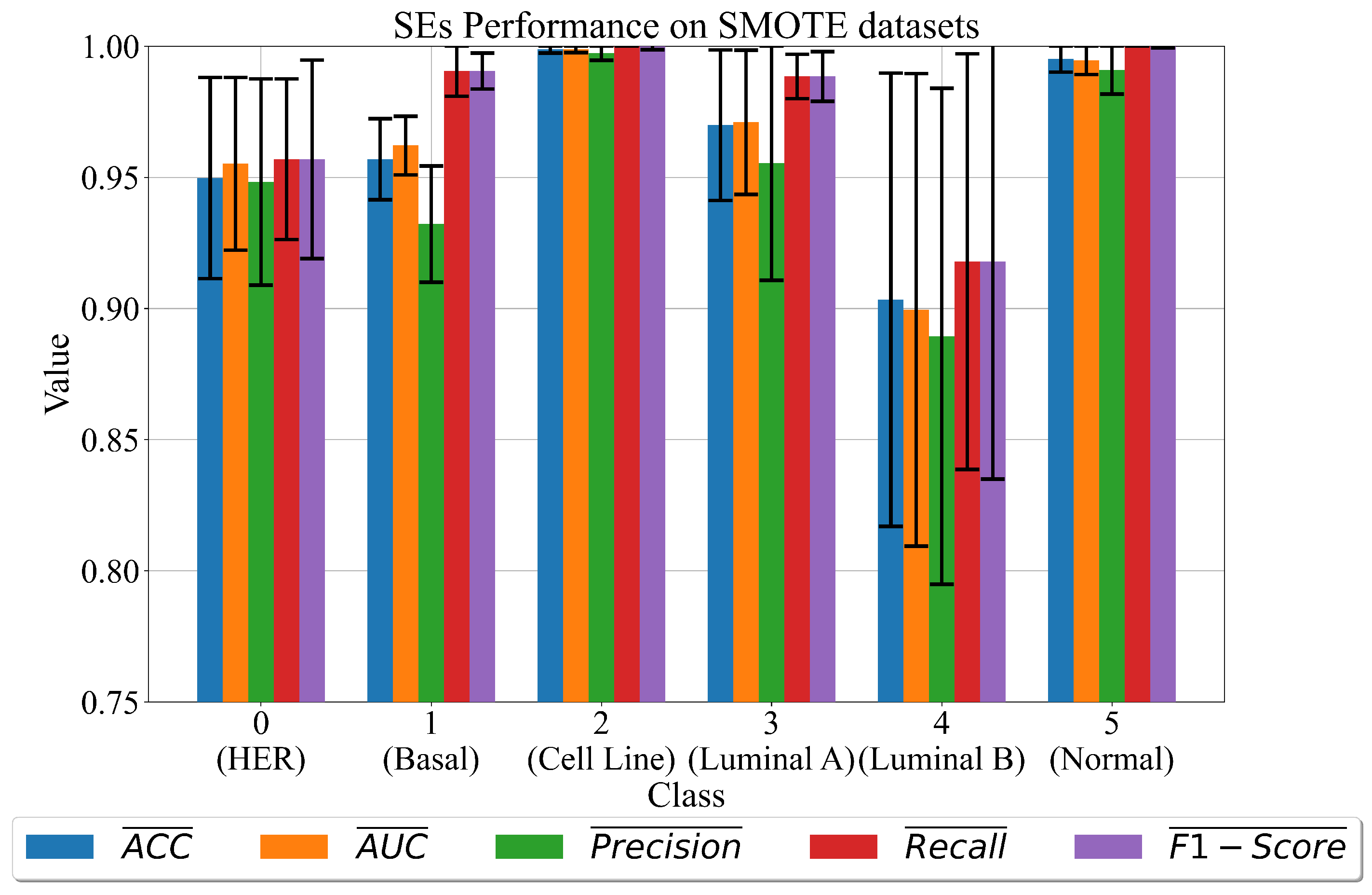
3.2. The Best Set of SEs Obtained on Dataset Balanced with SMOTE
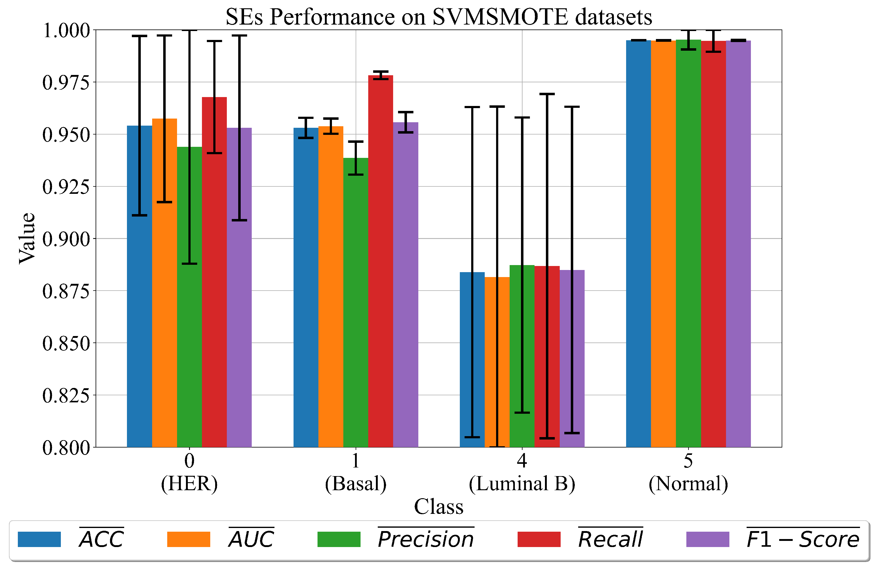
3.3. The Best Set of SEs Obtained on Dataset Balanced with SVMSMOTE
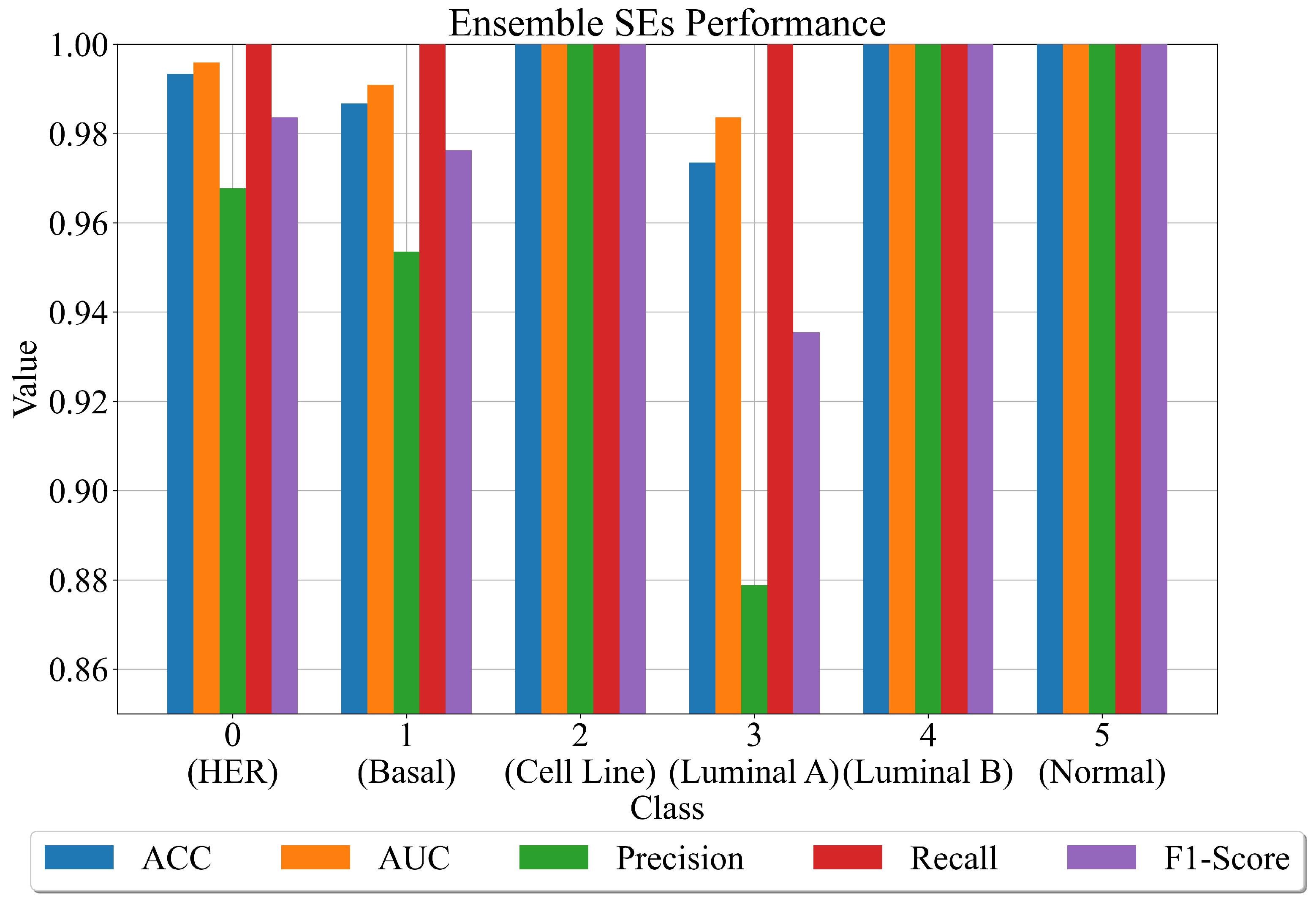
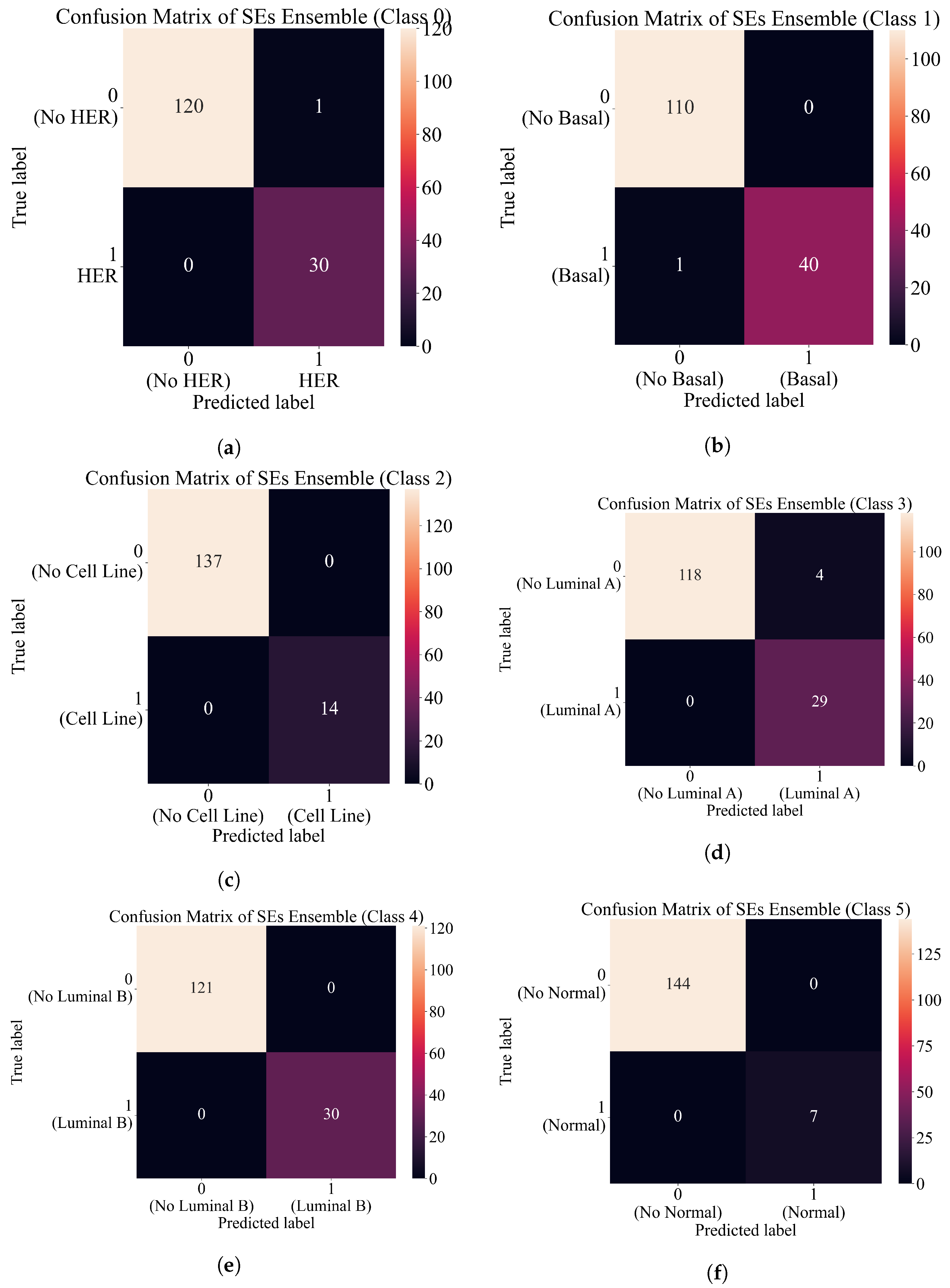
3.4. Final Evaluation on the Original Dataset
- First approach—using sets of the best SEs to create an ensemble.
- Second approach—combine the outputs of the best SEs with the original dataset and use the dataset to train the decision tree classifier.
- For each SE in the ensemble provides input variable values to calculate the output. Use this output in the Sigmoid function (Equation (2)) to determine the binary value (0 or 1).
- Combines the output of all SEs for a class into one output. If there are 40 SEs for one class, i.e., 30 output values of at least half of the generated output values must be the same value so that the final output is correctly classified.
- After the combination of all ensemble SE outputs into one output array, apply ACC, AUC, precision, recall, and F1-score to compute the evaluation metric performance.
4. Discussion
5. Conclusions
- The dimensionality reduction method (PCA) can greatly reduce the number of input dataset variables.
- The oversampling methods have a great influence on the performance of the GPSC since high accuracy of the obtained SEs was achieved.
- The proposed methodology of training using the 5CV method generated a large set of SEs, and in combination with the decision tree, the classifier contributed to the robust system, which could be used for the accurate classification of the breast cancer type.
- The application of the developed RHVS method proved to be crucial in finding the optimal hyperparameter combination on each oversampled dataset and obtaining SEs obtained with this combination of GPSC hyperparameters achieved high classification accuracy.
- The method is great for solving datasets with a large number of input variables and a small number of samples.
- The benefit of utilizing the GPSC method is that after each training round, a SE is obtained that is easier to understand and process, i.e., requires low computational resources.
- The benefit of utilizing different oversampling methods is to obtain multiple sets of symbolic expressions, which could potentially solve overfitting that can occur due to the small number of dataset samples.
- Although the number of input dataset variables is reduced, the large number of dataset oversampling variations can prolong the time required to train GPSC on each dataset.
- The RHVS method found the optimal combination of GPSC hyperparameters on each oversampled dataset variation, which means each time a new dataset variation was utilized, a RHVS method was used to find the combination of hyperparameters for that dataset variation.
- Generally, a long time was required to find the optimal combination of GPSC hyperparameters using the RHVS method.
Author Contributions
Funding
Institutional Review Board Statement
Informed Consent Statement
Data Availability Statement
Conflicts of Interest
Appendix A. Modification of Mathematical Functions
Appendix B. SEs Obtained in This Research
- Use the initial dataset, perform standard scaling and the PCA dimensionality reduction method to obtain 144 input variables. Transform the target variable from string to integer form using ordinal encoder and then one-hot encoder to binarize each class integer, creating one array for each class (one-versus-rest approach).
- Use the dataset to calculate the output for each SE and use that output as the input value in the sigmoid function (Equation (2)) to determine the output class (0 or 1).
References
- Feltes, B.C.; Chandelier, E.B.; Grisci, B.I.; Dorn, M. Cumida: An extensively curated microarray database for benchmarking and testing of machine learning approaches in cancer research. J. Comput. Biol. 2019, 26, 376–386. [Google Scholar] [CrossRef] [PubMed]
- Grisci, B.I.; Feltes, B.C.; Dorn, M. Neuroevolution as a tool for microarray gene expression pattern identification in cancer research. J. Biomed. Inform. 2019, 89, 122–133. [Google Scholar] [CrossRef] [PubMed]
- Karthik, D.; Kalaiselvi, K. MRMR-GWICA: A hybrid gene selection and ensemble clustering framework for breast cancer gene expression data. AIP Conf. Proc. 2022, 2393, 020064. [Google Scholar]
- Hamim, M.; El Moudden, I.; Pant, M.D.; Moutachaouik, H.; Hain, M. A hybrid gene selection strategy based on fisher and ant colony optimization algorithm for breast cancer classification. Int. J. Online Biomed. Eng. 2021, 17, 148–163. [Google Scholar] [CrossRef]
- Afif, G.G.; Astuti, W. Cancer Detection based on Microarray Data Classification Using FLNN and Hybrid Feature Selection. J. Resti (Rekayasa Sist. Dan Teknol. Informasi) 2021, 5, 794–801. [Google Scholar] [CrossRef]
- Tang, W.; Wan, S.; Yang, Z.; Teschendorff, A.E.; Zou, Q. Tumor origin detection with tissue-specific miRNA and DNA methylation markers. Bioinformatics 2018, 34, 398–406. [Google Scholar] [CrossRef] [PubMed] [Green Version]
- Jain, I.; Jain, V.K.; Jain, R. Correlation feature selection based improved-binary particle swarm optimization for gene selection and cancer classification. Appl. Soft Comput. 2018, 62, 203–215. [Google Scholar] [CrossRef]
- Shukla, A.K.; Singh, P.; Vardhan, M. A two-stage gene selection method for biomarker discovery from microarray data for cancer classification. Chemom. Intell. Lab. Syst. 2018, 183, 47–58. [Google Scholar] [CrossRef]
- Lu, H.; Chen, J.; Yan, K.; Jin, Q.; Xue, Y.; Gao, Z. A hybrid feature selection algorithm for gene expression data classification. Neurocomputing 2017, 256, 56–62. [Google Scholar] [CrossRef]
- Mohapatra, P.; Chakravarty, S.; Dash, P. Microarray medical data classification using kernel ridge regression and modified cat swarm optimization based gene selection system. Swarm Evol. Comput. 2016, 28, 144–160. [Google Scholar] [CrossRef]
- Shreem, S.S.; Abdullah, S.; Nazri, M.Z.A. Hybrid feature selection algorithm using symmetrical uncertainty and a harmony search algorithm. Int. J. Syst. Sci. 2016, 47, 1312–1329. [Google Scholar] [CrossRef]
- Alromema, N.; Syed, A.H.; Khan, T. A Hybrid Machine Learning Approach to Screen Optimal Predictors for the Classification of Primary Breast Tumors from Gene Expression Microarray Data. Diagnostics 2023, 13, 708. [Google Scholar] [CrossRef] [PubMed]
- Grisci, B. Breast Cancer Gene Expression—Cumida. 2020. Available online: https://www.kaggle.com/datasets/brunogrisci/breast-cancer-gene-expression-cumida (accessed on 15 April 2023).
- Abdi, H.; Williams, L.J. Principal component analysis. Wiley Interdiscip. Rev. Comput. Stat. 2010, 2, 433–459. [Google Scholar] [CrossRef]
- Pedregosa, F.; Varoquaux, G.; Gramfort, A.; Michel, V.; Thirion, B.; Grisel, O.; Blondel, M.; Prettenhofer, P.; Weiss, R.; Dubourg, V.; et al. Scikit-learn: Machine learning in Python. J. Mach. Learn. Res. 2011, 12, 2825–2830. [Google Scholar]
- Bertucci, F.; Finetti, P.; Birnbaum, D. Basal breast cancer: A complex and deadly molecular subtype. Curr. Mol. Med. 2012, 12, 96–110. [Google Scholar] [CrossRef] [Green Version]
- Loibl, S.; Gianni, L. HER2-positive breast cancer. Lancet 2017, 389, 2415–2429. [Google Scholar] [CrossRef]
- Ades, F.; Zardavas, D.; Bozovic-Spasojevic, I.; Pugliano, L.; Fumagalli, D.; De Azambuja, E.; Viale, G.; Sotiriou, C.; Piccart, M. Luminal B breast cancer: Molecular characterization, clinical management, and future perspectives. J. Clin. Oncol. 2014, 32, 2794–2803. [Google Scholar] [CrossRef] [Green Version]
- Ciriello, G.; Sinha, R.; Hoadley, K.A.; Jacobsen, A.S.; Reva, B.; Perou, C.M.; Sander, C.; Schultz, N. The molecular diversity of Luminal A breast tumors. Breast Cancer Res. Treat. 2013, 141, 409–420. [Google Scholar] [CrossRef] [Green Version]
- Dai, X.; Cheng, H.; Bai, Z.; Li, J. Breast cancer cell line classification and its relevance with breast tumor subtyping. J. Cancer 2017, 8, 3131. [Google Scholar] [CrossRef] [Green Version]
- Brownlee, J. Data Preparation for Machine Learning: Data Cleaning, Feature Selection, and Data Transforms in Python; Machine Learning Mastery: San Francisco, CA, USA, 2020. [Google Scholar]
- Han, H.; Wang, W.Y.; Mao, B.H. Borderline-SMOTE: A new over-sampling method in imbalanced data sets learning. In Advances in Intelligent Computing, Proceedings of the International Conference on Intelligent Computing, ICIC 2005, Hefei, China, 23–26 August 2005; Springer: Berlin/Heidelberg, Germany, 2005; Part 1; pp. 878–887. [Google Scholar]
- Fernández, A.; Garcia, S.; Herrera, F.; Chawla, N.V. SMOTE for learning from imbalanced data: Progress and challenges, marking the 15-year anniversary. J. Artif. Intell. Res. 2018, 61, 863–905. [Google Scholar] [CrossRef]
- Nguyen, H.M.; Cooper, E.W.; Kamei, K. Borderline over-sampling for imbalanced data classification. Int. J. Knowl. Eng. Soft Data Paradig. 2011, 3, 4–21. [Google Scholar] [CrossRef] [Green Version]
- Priyanka; Kumar, D. Decision tree classifier: A detailed survey. Int. J. Inf. Decis. Sci. 2020, 12, 246–269. [Google Scholar] [CrossRef]
- Anđelić, N.; Baressi Šegota, S.; Glučina, M.; Lorencin, I. Classification of Faults Operation of a Robotic Manipulator Using Symbolic Classifier. Appl. Sci. 2023, 13, 1962. [Google Scholar] [CrossRef]
- Anđelić, N.; Baressi Šegota, S.; Glučina, M.; Car, Z. Estimation of Interaction Locations in Super Cryogenic Dark Matter Search Detectors Using Genetic Programming-Symbolic Regression Method. Appl. Sci. 2023, 13, 2059. [Google Scholar] [CrossRef]
- Sokolova, M.; Japkowicz, N.; Szpakowicz, S. Beyond accuracy, F-score and ROC: A family of discriminant measures for performance evaluation. In AI 2006: Advances in Artificial Intelligence, Proceedings of the 19th Australian Joint Conference on Artificial Intelligence, Hobart, Australia, 4–8 December 2006; Proceedings 19; Springer: Berlin/Heidelberg, Germany, 2006; pp. 1015–1021. [Google Scholar]
- Davis, J.; Goadrich, M. The relationship between Precision-Recall and ROC curves. In Proceedings of the 23rd International Conference on Machine Learning, Pittsburgh, PA, USA, 25–29 June 2006; pp. 233–240. [Google Scholar]
- Goutte, C.; Gaussier, E. A probabilistic interpretation of precision, recall and F-score, with implication for evaluation. In Advances in Information Retrieval, Proceedings of the 27th European Conference on IR Research, ECIR 2005, Santiago de Compostela, Spain, 21–23 March 2005; Proceedings 27; Springer: Berlin/Heidelberg, Germany, 2005; pp. 345–359. [Google Scholar]


| Reference | Reduction Methods | AI Methods | Results |
|---|---|---|---|
| [4] | ACOC5 | DT, SVM, KNN, RF | ACC: 0.954 |
| [5] | IGAG | FLNN | ACC: 0.856 |
| [6] | MRMD, PCA | RFC | ACC: 0.913 |
| [7] | CFS-PSO | Naive-Bayes | ACC: 0.927 |
| [8] | CMIM-AGA | ELM, SVM, KNN | ACC:0.903 |
| [9] | MIMAGA | ELM | ACC:0.952 |
| [10] | MCSO | RR, OSRR, SVMRBF, SVM Poly, and KRR | ACC: 0.966 |
| [11] | SUF-HSA | IBL | ACC: 0.833 |
| [12] | hybrid Feature Selection sequential framework consisting of minimum Redundancy-Maximum Relevance, two-tailed unpaired t-test, and meta-heuristics | SVM, KNN, ANN, NB, DT, XGBoost | ACC: 0.976 |
| Class Original Name | Integer Representation |
|---|---|
| HER | 0 |
| basal | 1 |
| cell_line | 2 |
| luminal A | 3 |
| luminal B | 4 |
| normal | 5 |
| Class Labels | Label 0 | Label 1 |
|---|---|---|
| 0 | 121 | 30 |
| 1 | 110 | 41 |
| 2 | 137 | 14 |
| 3 | 122 | 29 |
| 4 | 121 | 30 |
| 5 | 144 | 7 |
| Oversampling Method | Class 0 vs. Rest | Class 1 vs. Rest | Class 2 vs. Rest | Class 3 vs. Rest | Class 4 vs. Rest | Class 5 vs. Rest |
|---|---|---|---|---|---|---|
| Original Dataset | 30, 120 | 41, 110 | 14, 137 | 29, 122 | 30, 121 | 7, 144 |
| BorderlineSMOTE | 121, 121 | 110, 110 | 14, 137 | 29, 122 | 121, 121 | 141, 141 |
| SMOTE | 121, 121 | 110, 110 | 137, 137 | 122, 122 | 121, 121 | 144, 144 |
| SVMSMOTE | 121, 121 | 110, 110 | 69, 137 | 71, 122 | 121, 121 | 144, 144 |
| DTC Hyperparameter | Value |
|---|---|
| criterion | ‘gini’ |
| splitter | best |
| max_depth | None |
| min_samples_split | 2 |
| Dataset Class | GPSC Hyperparameters | SEs Length | Average Length |
|---|---|---|---|
| 0 | 1305, 286, 320, (6, 12), 0.027, 0.92, 0.0034, 0.047, 0.000849, 0.992, (, 6538.77), | 57/106/109/61/59 | 78.4 |
| 1 | 1773, 255,115,(5, 15), 0.028, 0.95, 0.013, 0.001, 0.000761, 0.99, (, 3.62), | 51/66/91/100/304 | 122.4 |
| 4 | 1467, 208, 206, (7, 14), 0.028, 0.95, 0.0067, 0.013, 0.00067, 0.998, (, 9994.33), | 86/214/140/92/144 | 135.2 |
| 5 | 1636, 208, 235, (6, 14), 0.013, 0.95, 0.027, 0.0014, 0.00047, 0.99, (, 2091.41), | 74/17/25/11/7 | 26.8 |
| Dataset Class | GPSC Hyperparameters | SEs Length | Average Length |
|---|---|---|---|
| 0 | 1689, 242, 229, (7, 9), 0.021, 0.95, 0.024, 0.0018, 0.000128, 0.9999, (, 4881.51), | 322/99/103/70/28 | 124.4 |
| 1 | 1333, 238, 492, (5, 18), 0.015, 0.9, 0.058, 0.02, 0.000257, 0.99, (, 9422.75), | 68/42/82/34/82 | 61.6 |
| 2 | 1981, 242, 322, (4, 16), 0.034, 0.9, 0.0036, 0.06, 0.000926, 0.99, (, 606.08), | 82/18/21/22/86 | 45.8 |
| 3 | 1927, 284, 196, (7, 14), 0.18, 0.52, 0.026, 0.25, 0.0009, 0.99, (, 7889.12) | 77/128/42/57/33 | 67.4 |
| 4 | 1587, 285, 170, (7, 10), 0.044, 0.032, 0.095, 0.82, 0.000912, 0.99, (, 7425.75), | 391/944/191/155/81 | 352.4 |
| 5 | 1818, 292, 179, (7, 18), 0.045, 0.93, 0.0084, 0.012, 0.000295, 0.99, (, 7910.95), | 27/18/51/18/17 | 26.2 |
| Dataset Class | GPSC Hyperparameters | SEs Length | Average Length |
|---|---|---|---|
| 0 | 1487, 226, 140, (7, 18), 0.015, 0.95, 0.011, 0.017, 0.000373, 0.99, (, 2732.52), | 47/41/58/98/82 | 65.2 |
| 1 | 1384, 213, 429, (5, 16), 0.013, 0.96, 0.017, 0.003, 0.000193, 0.99, (, 4173.5), | 249/66/103/302/185 | 181 |
| 4 | 1393, 201, 113, (4, 8), 0.017, 0.97, 0.0019, 0.0027, 0.000675, 0.99, (, 7489.67), | 138/52/68/294/147 | 138.8 |
| 5 | 1263, 211, 103, (6, 9), 0.011, 0.92, 0.06, 0.0034, 0.00028, 0.99, (, 5345.63), | 96/10/11/91/77 | 57 |
| Evaluation Metric | Value |
|---|---|
| 0.992 | |
| 0.995 | |
| 0.966 | |
| 1.0 | |
| 0.9825 |
| Evaluation Metric | Value |
|---|---|
| 0.994 | |
| 0.993 | |
| 0.984 | |
| 0.99 | |
| 0.987 |
| Reference | Reduction Methods | AI Methods | Results |
|---|---|---|---|
| [4] | ACOC5 | DT, SVM, KNN, RF | ACC: 0.954 |
| [5] | IGAG | FLNN | ACC: 0.856 |
| [6] | MRMD, PCA | RFC | ACC: 0.913 |
| [7] | CFS-PSO | Naive-Bayes | ACC: 0.927 |
| [8] | CMIM-AGA | ELM, SVM, KNN | ACC: 0.903 |
| [9] | MIMAGA | ELM | ACC: 0.952 |
| [10] | MCSO | RR, OSRR, SVMRBF, SVM Poly, and KRR | ACC: 0.966 |
| [11] | SUF-HSA | IBL | ACC: 0.833 |
| [12] | hybrid Feature Selection sequential framework consisting of minimum Redundancy-Maximum Relevance, two-tailed unpaired t-test, and meta-heuristics | SVM, KNN, ANN, NB, DT, XGBoost | ACC: 0.976 |
| This paper | PCA + oversampling methods (BorderlineSMOTE, SMOTE, and SVMSMOTE) | GPSC GPSC + DTC | ACC: 0.992 ACC: 0.994 |
Disclaimer/Publisher’s Note: The statements, opinions and data contained in all publications are solely those of the individual author(s) and contributor(s) and not of MDPI and/or the editor(s). MDPI and/or the editor(s) disclaim responsibility for any injury to people or property resulting from any ideas, methods, instructions or products referred to in the content. |
© 2023 by the authors. Licensee MDPI, Basel, Switzerland. This article is an open access article distributed under the terms and conditions of the Creative Commons Attribution (CC BY) license (https://creativecommons.org/licenses/by/4.0/).
Share and Cite
Anđelić, N.; Baressi Šegota, S. Development of Symbolic Expressions Ensemble for Breast Cancer Type Classification Using Genetic Programming Symbolic Classifier and Decision Tree Classifier. Cancers 2023, 15, 3411. https://doi.org/10.3390/cancers15133411
Anđelić N, Baressi Šegota S. Development of Symbolic Expressions Ensemble for Breast Cancer Type Classification Using Genetic Programming Symbolic Classifier and Decision Tree Classifier. Cancers. 2023; 15(13):3411. https://doi.org/10.3390/cancers15133411
Chicago/Turabian StyleAnđelić, Nikola, and Sandi Baressi Šegota. 2023. "Development of Symbolic Expressions Ensemble for Breast Cancer Type Classification Using Genetic Programming Symbolic Classifier and Decision Tree Classifier" Cancers 15, no. 13: 3411. https://doi.org/10.3390/cancers15133411