
Deep Neural Networks and Machine Learning Radiomics Modelling for Prediction of Relapse in Mantle Cell Lymphoma

 , , , and
Abstract
:Simple Summary
Abstract
1. Introduction
2. Materials and Methods
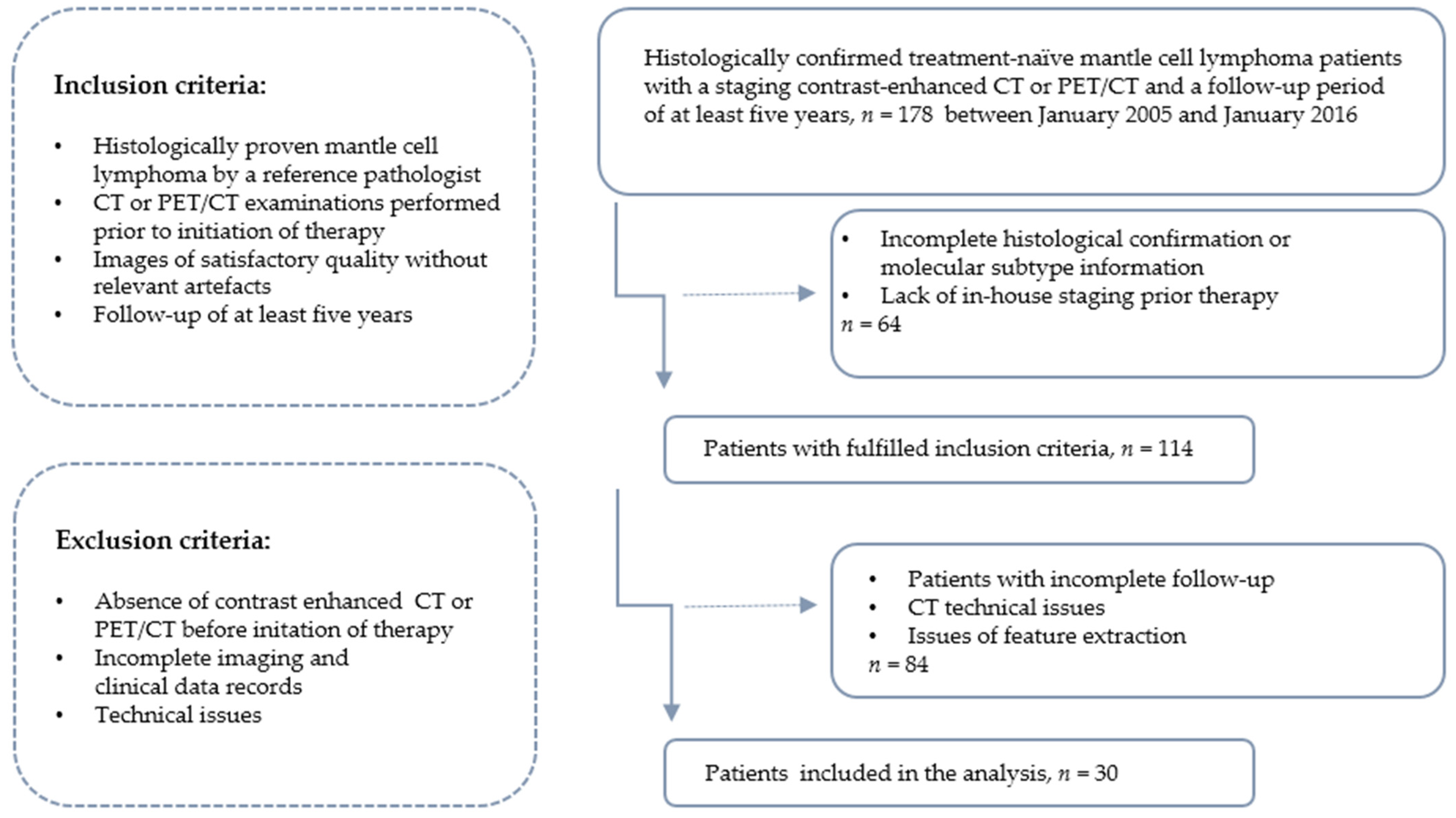
2.1. Patients and Imaging Protocol
2.2. Radiomic-Based Machine Learning as Prediction Model
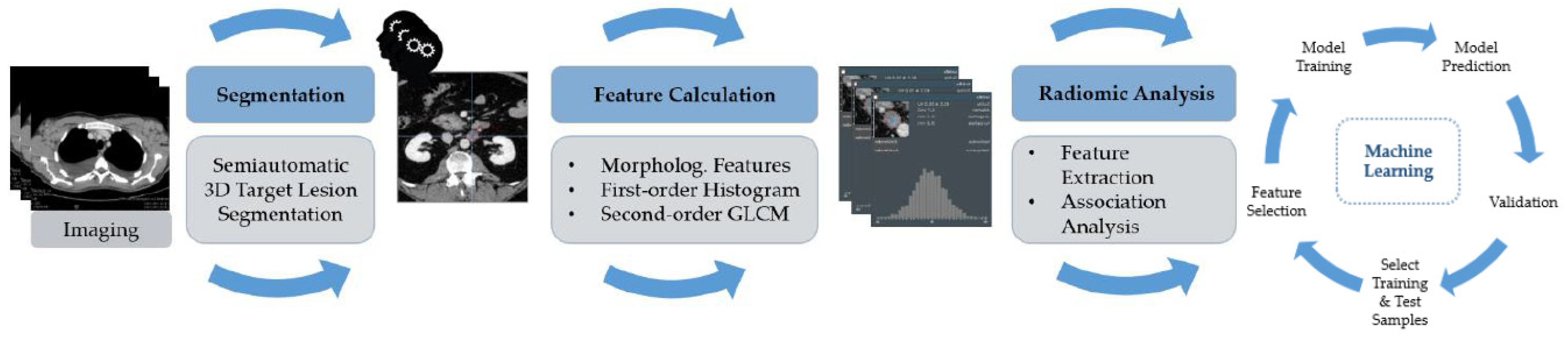
2.2.1. Tumour Segmentation, Data Processing and Feature Extraction
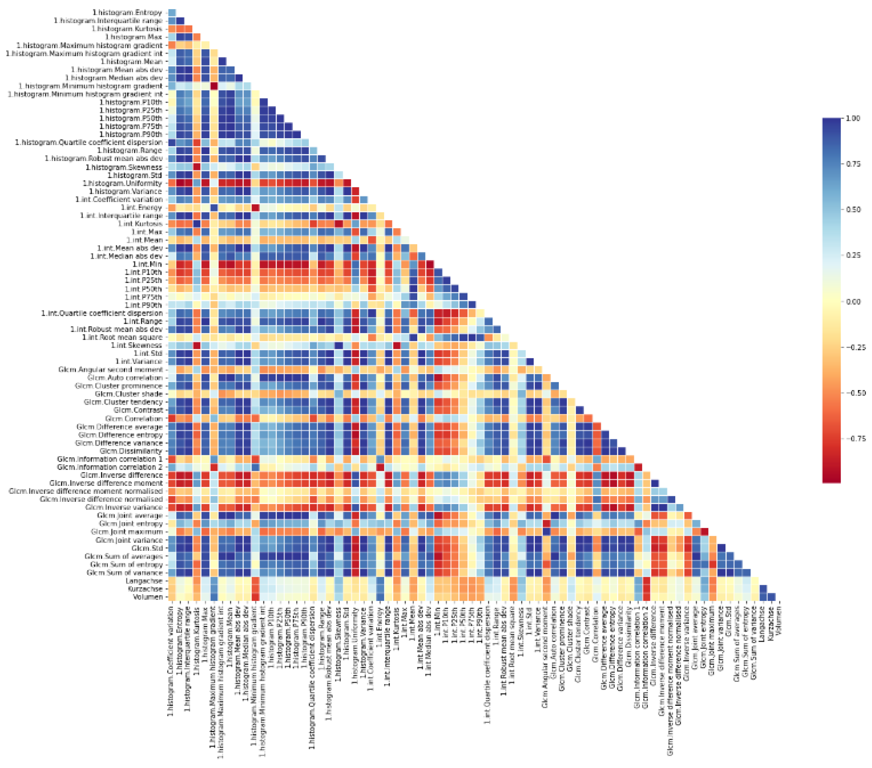
2.2.2. Features Selection
2.2.3. Dataset Characteristics and Preprocessing
2.2.4. Machine Learning (ML) Classification Architectures
2.2.5. ML Model Development and Evaluation
2.3. Neural Network Approach as Prediction Model
2.3.1. Dataset, Training and Validation
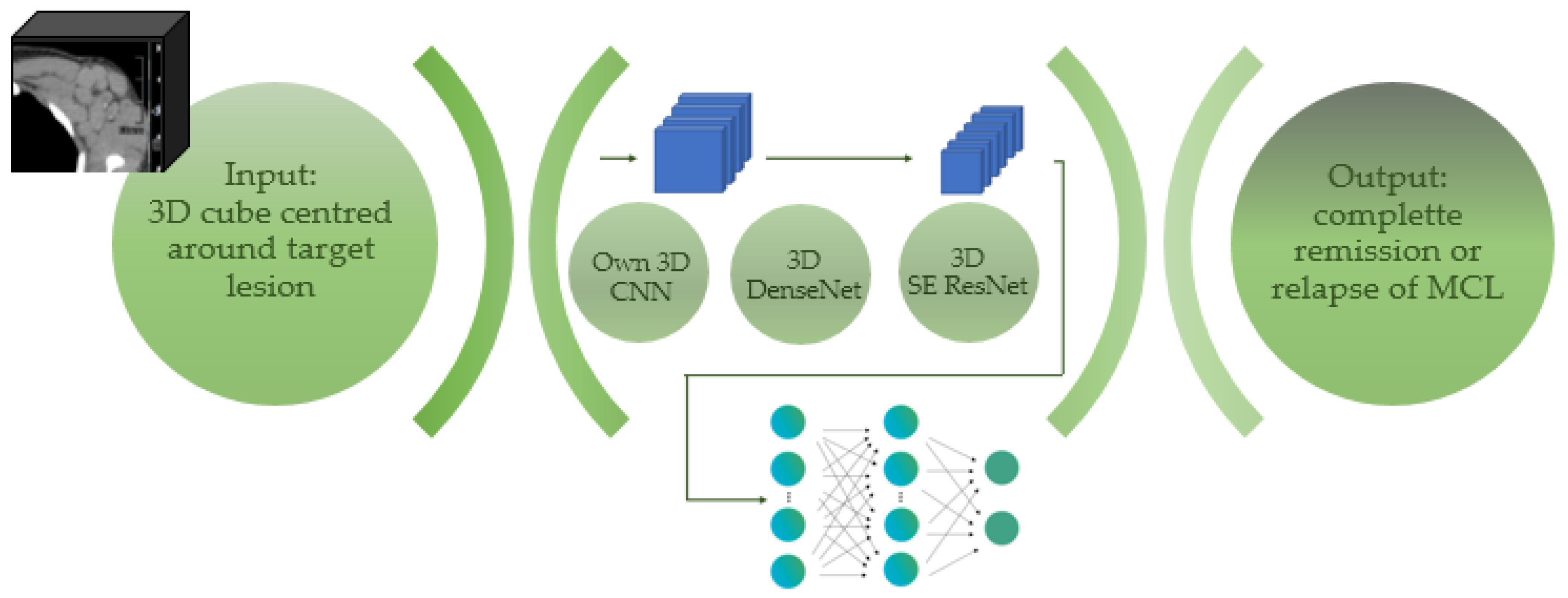
2.3.2. Deep CNN Architecture
3. Results
3.1. Patient Characteristics
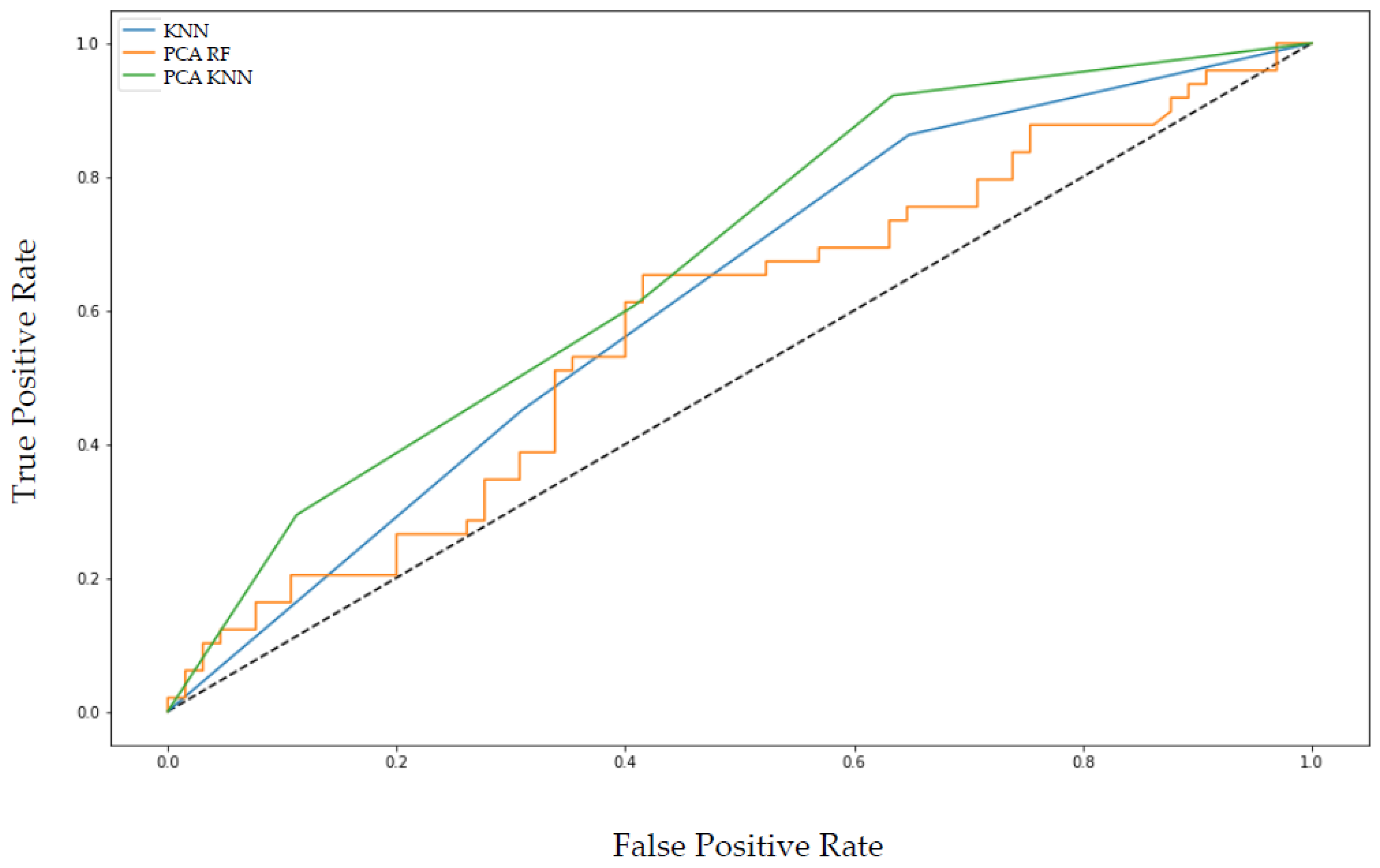
3.2. Radiomic Analysis and the Machine Learning Prediction Model
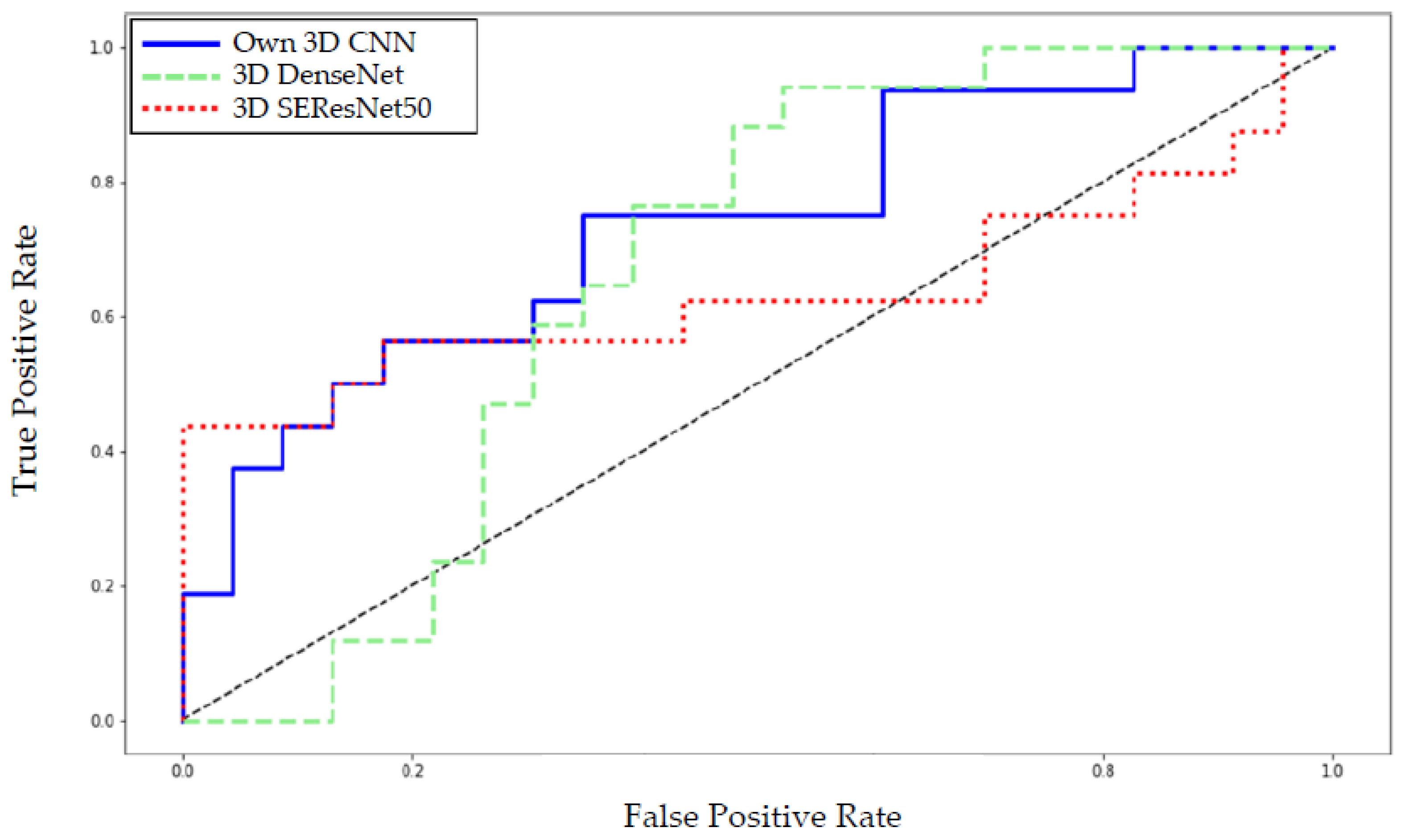
3.3. The CNN-Based Neural Network Approach as Prediction Model
3.4. Comparing the Deep Neural Network with the Machine Learning Approach
4. Discussion
5. Conclusions
Author Contributions
Funding
Institutional Review Board Statement
Informed Consent Statement
Data Availability Statement
Conflicts of Interest
Appendix A

| Setting | Determination |
|---|---|
| Bin Method | FBS |
| Bin Amount | 1 |
| LoG Filter | 0 |
| LoG Sigma | 1 |
| Matrix Aggregation Method | 3D Average Directions |
| Resample Filter | 0 |
| Resample Spacing X | 1 |
| Resample Spacing Y | 1 |
| Resample Spacing Z | 0 |
| Second-Order Distance | 1 |
| Threshold Filter | 0 |
| Threshold Filter Min | −1000 |
| Threshold Filter Max | 3000 |
| Radiomic Features of First Order: Histogram | Radiomic Features of Second Order: Gray Level Co-Occurrence Matrix (GLCM) |
|---|---|
| Skewness | Angular Second Moment |
| Uniformity | Autocorrelation |
| Entropy | Correlation |
| Kurtosis | Contrast |
| Minimum Histogram Gradient | Energy |
| Maximum Histogram Gradient | Joint Average |
| Coefficient Variation | Sum Average |
| Quartile Coefficient Dispersion | Joint Maximum |
| P 10th (10th percentile) | Joint Entropy |
| P 25th (25th percentile) | Sum Entropy |
| P 50th (50th percentile) | Difference Entropy |
| P 90th (90th percentile) | Cluster Prominence |
| Interquartile Range | Cluster Shade |
| Minimum | Cluster Tendency |
| Maximum | Information Correlation |
| Mean | Information Correlation Difference |
| Mean Absolute Deviation | Inverse Difference |
| Median Absolute Deviation | Inverse Difference Normalised |
| Range | Inverse Difference Moment |
| Root Mean Square | Inverse Difference Moment Normalised |
| Standard Deviation | Difference Average |
| Variance | Difference Variance |
| Dissimilarity | |
| Inverse Variance | |
| Joint Variance | |
| Sum Variance |
References
- Epperla, N.; Hamadani, M.; Fenske, T.S.; Costa, L.J. Incidence and survival trends in mantle cell lymphoma. Br. J. Haematol. 2017, 181, 703–706. [Google Scholar] [CrossRef] [PubMed] [Green Version]
- Swerdlow, S.H.; Campo, E.; Pileri, S.A.; Harris, N.L.; Stein, H.; Siebert, R.; Advani, R.; Ghielmini, M.; Salles, G.A.; Zelenetz, A.D.; et al. The 2016 revision of the World Health Organization classification of lymphoid neoplasms. Blood 2016, 127, 2375–2390. [Google Scholar] [CrossRef] [PubMed] [Green Version]
- Kienle, D.; Katzenberger, T.; Ott, G.; Saupe, D.; Benner, A.; Kohlhammer, H.; Barth, T.F.; Höller, S.; Kalla, J.; Rosenwald, A.; et al. Quantitative gene expression deregulation in mantle-cell lymphoma: Correlation with clinical and biologic factors. J. Clin. Oncol. 2007, 25, 2770–2777. [Google Scholar] [CrossRef] [PubMed]
- Rosenwald, A.; Wright, G.; Wiestner, A.; Chan, W.C.; Connors, J.M.; Campo, E.; Gascoyne, R.D.; Grogan, T.M.; Muller-Hermelink, H.K.; Smeland, E.B.; et al. The proliferation gene expression signature is a quantitative integrator of oncogenic events that predicts survival in mantle cell lymphoma. Cancer Cell 2003, 3, 185–197. [Google Scholar] [CrossRef] [Green Version]
- Salaverria, I.; Zettl, A.; Beà, S.; Moreno, V.; Valls, J.; Hartmann, E.; Ott, G.; Wright, G.; Lopez-Guillermo, A.; Chan, W.C.; et al. Specific secondary genetic alterations in mantle cell lymphoma provide prognostic information independent of the gene expression–based proliferation signature. J. Clin. Oncol. 2007, 25, 1216–1222. [Google Scholar] [CrossRef]
- Tiemann, M.; Schrader, C.; Klapper, W.; Dreyling, M.H.; Campo, E.; Norton, A.; Berger, F.; Kluin, P.; Ott, G.; Pileri, S.; et al. Histopathology, cell proliferation indices and clinical outcome in 304 patients with mantle cell lymphoma (MCL): A clinicopathological study from the European MCL Network. Br. J. Haematol. 2005, 131, 29–38. [Google Scholar] [CrossRef]
- Dreyling, M.; Campo, E.; Hermine, O.; Jerkeman, M.; le Gouill, S.; Rule, S.; Shpilberg, O.; Walewski, J.; Ladetto, M. Newly diagnosed and relapsed mantle cell lymphoma: ESMO Clinical Practice Guidelines for diagnosis, treatment and follow-up. Ann. Oncol. 2017, 28, iv62–iv71. [Google Scholar] [CrossRef]
- Swerdlow, S.H.; Campo, E.; Harris, N.L.; Jaffe, E.S.; Pileri, S.A.; Stein, H.; Thiele, J.; Vardiman, J.W. WHO Classification of Tumours of Haematopoietic and Lymphoid Tissues. WHO Classification of Tumours, 4th ed.; WHO Press: Geneva, Switzerland, 2017; Volume 2. [Google Scholar]
- Geisler, C.H.; Kolstad, A.; Laurell, A.; Andersen, N.S.; Pedersen, L.B.; Jerkeman, M.; Eriksson, M.; Nordström, M.; Kimby, E.; Boesen, A.M. Long-term progression-free survival of mantle cell lymphoma after intensive front-line immu-nochemotherapy with in vivo–purged stem cell rescue: A nonrandomized phase 2 multicenter study by the Nordic Lymphoma Group. Blood. J. Am. Soc. Hematol. 2008, 112, 2687–2693. [Google Scholar]
- Cook, G.J.R.; Goh, V. What can artificial intelligence teach us about the molecular mechanisms underlying disease? Eur. J. Pediatr. 2019, 46, 2715–2721. [Google Scholar] [CrossRef] [Green Version]
- Lambin, P.; Rios-Velazquez, E.; Leijenaar, R.; Carvalho, S.; van Stiphout, R.G.P.M.; Granton, P.; Zegers, C.M.L.; Gillies, R.; Boellard, R.; Dekker, A.; et al. Radiomics: Extracting more information from medical images using advanced feature analysis. Eur. J. Cancer 2012, 48, 441–446. [Google Scholar] [CrossRef] [Green Version]
- Lambin, P.; Leijenaar, R.T.H.; Deist, T.M.; Peerlings, J.; de Jong, E.E.C.; van Timmeren, J.; Sanduleanu, S.; Larue, R.T.H.M.; Even, A.J.G.; Jochems, A.; et al. Radiomics: The bridge between medical imaging and personalized medicine. Nat. Rev. Clin. Oncol. 2017, 14, 749–762. [Google Scholar] [CrossRef] [PubMed]
- Schieber, M.; Gordon, L.I.; Karmali, R. Current overview and treatment of mantle cell lymphoma. F1000Research 2018, 7, 1136. [Google Scholar] [CrossRef] [PubMed]
- Hill, H.A.; Qi, X.; Jain, P.; Nomie, K.; Wang, Y.; Zhou, S.; Wang, M.L. Genetic mutations and features of mantle cell lymphoma: A systematic review and meta-analysis. Blood Adv. 2020, 4, 2927–2938. [Google Scholar] [CrossRef] [PubMed]
- Nadeu, F.; Martin-Garcia, D.; Clot, G.; Díaz-Navarro, A.; Duran-Ferrer, M.; Navarro, A.; Vilarrasa-Blasi, R.; Kulis, M.; Royo, R.; Gutiérrez-Abril, J.; et al. Genomic and epigenomic insights into the origin, pathogenesis, and clinical behavior of mantle cell lymphoma subtypes. Blood 2020, 136, 1419–1432. [Google Scholar] [CrossRef] [PubMed]
- Hoster, E.; Dreyling, M.; Klapper, W.; Gisselbrecht, C.; Van Hoof, A.; Kluin-Nelemans, J.C.; Pfreundschuh, M.; Reiser, M.; Metzner, B.; Einsele, H.; et al. A new prognostic index (MIPI) for patients with advanced-stage mantle cell lymphoma. Blood 2008, 111, 558–565. [Google Scholar] [CrossRef] [PubMed]
- Hoster, E.; Rosenwald, A.; Berger, F.; Bernd, H.-W.; Hartmann, S.; Loddenkemper, C.; Barth, T.F.; Brousse, N.; Pileri, S.; Rymkiewicz, G.; et al. Prognostic value of Ki-67 index, cytology, and growth pattern in mantle-cell lymphoma: Results from randomized trials of the European Mantle Cell Lymphoma Network. J. Clin. Oncol. 2016, 34, 1386–1394. [Google Scholar] [CrossRef] [PubMed]
- Ladetto, M.; Magni, M.; Pagliano, G.; De Marco, F.; Drandi, D.; Ricca, I.; Astolfi, M.; Matteucci, P.; Guidetti, A.; Mantoan, B.; et al. Rituximab induces effective clearance of minimal residual disease in molecular relapses of mantle cell lymphoma. Biol. Blood Marrow Transplant. 2006, 12, 1270–1276. [Google Scholar] [CrossRef] [Green Version]
- Pott, C.; Hoster, E.; Delfau-Larue, M.-H.; Beldjord, K.; Böttcher, S.; Asnafi, V.; Plonquet, A.; Siebert, R.; Callet-Bauchu, E.; Andersen, N.; et al. Molecular remission is an independent predictor of clinical outcome in patients with mantle cell lymphoma after combined immunochemotherapy: A European MCL intergroup study. Blood 2010, 115, 3215–3223. [Google Scholar] [CrossRef]
- Martin, P.; Chadburn, A.; Christos, P.; Weil, K.; Furman, R.R.; Ruan, J.; Elstrom, R.; Niesvizky, R.; Ely, S.; DiLiberto, M. Outcome of deferred initial therapy in mantle-cell lymphoma. J. Clin. Oncol. 2009, 27, 1209–1213. [Google Scholar] [CrossRef]
- Steinbuss, G.; Kriegsmann, M.; Zgorzelski, C.; Brobeil, A.; Goeppert, B.; Dietrich, S.; Mechtersheimer, G.; Kriegsmann, K. Deep Learning for the Classification of Non-Hodgkin Lymphoma on Histopathological Images. Cancers 2021, 13, 2419. [Google Scholar] [CrossRef]
- Davnall, F.; Yip, C.S.P.; Ljungqvist, G.; Selmi, M.; Ng, F.; Sanghera, B.; Ganeshan, B.; Miles, K.A.; Cook, G.J.; Goh, V. Assessment of tumor heterogeneity: An emerging imaging tool for clinical practice? Insights Imaging 2012, 3, 573–589. [Google Scholar] [CrossRef] [PubMed] [Green Version]
- Burrell, R.A.; McGranahan, N.; Bartek, J.; Swanton, C. The causes and consequences of genetic heterogeneity in cancer evolution. Nature 2013, 501, 338–345. [Google Scholar] [CrossRef] [PubMed]
- Stanta, G.; Bonin, S. Overview on clinical relevance of intra-tumor heterogeneity. Front. Med. 2018, 5, 85. [Google Scholar] [CrossRef] [PubMed] [Green Version]
- Schürch, C.M.; Federmann, B.; Quintanilla-Martinez, L.; Fend, F. Tumor heterogeneity in lymphomas: A different breed. Pathobiology 2018, 85, 130–145. [Google Scholar] [CrossRef]
- Gillies, R.J.; Kinahan, P.E.; Hricak, H. Radiomics: Images are more than pictures, they are data. Radiology 2016, 278, 563–577. [Google Scholar] [CrossRef] [Green Version]
- Ibrahim, A.; Primakov, S.; Beuque, M.; Woodruff, H.; Halilaj, I.; Wu, G.; Refaee, T.; Granzier, R.; Widaatalla, Y.; Hustinx, R.; et al. Radiomics for precision medicine: Current challenges, future prospects, and the proposal of a new framework. Methods 2021, 188, 20–29. [Google Scholar] [CrossRef]
- Sollini, M.; Antunovic, L.; Chiti, A.; Kirienko, M. Towards clinical application of image mining: A systematic review on artificial intelligence and radiomics. Eur. J. Nucl. Med. Mol. Imaging 2019, 46, 2656–2672. Available online: https://link.springer.com/article/10.1007/s00259-019-04372-x (accessed on 17 December 2021). [CrossRef] [Green Version]
- Mayerhoefer, M.E.; Riedl, C.C.; Kumar, A.; Gibbs, P.; Weber, M.; Tal, I.; Schilksy, J.; Schöder, H. Radiomic features of glucose metabolism enable prediction of outcome in mantle cell lymphoma. Eur. J. Nucl. Med. Mol. Pediatr. 2019, 46, 2760–2769. [Google Scholar] [CrossRef] [Green Version]
- Limkin, E.J.; Reuzé, S.; Carré, A.; Sun, R.; Schernberg, A.; Alexis, A.; Deutsch, E.; Ferté, C.; Robert, C. The complexity of tumor shape, spiculatedness, correlates with tumor radiomic shape features. Sci. Rep. 2019, 9, 4329. [Google Scholar] [CrossRef] [Green Version]
- Jeong, W.K.; Jamshidi, N.; Felker, E.R.; Raman, S.S.; Lu, D.S. Radiomics and radiogenomics of primary liver cancers. Clin. Mol. Hepatol. 2019, 25, 21–29. [Google Scholar] [CrossRef]
- Horvat, N.; Bates, D.D.B.; Petkovska, I. Novel imaging techniques of rectal cancer: What do radiomics and radiogenomics have to offer? A literature review. Abdom. Radiol. 2019, 44, 3764–3774. [Google Scholar] [CrossRef] [PubMed]
- Lohmann, P.; Kocher, M.; Ceccon, G.; Bauer, E.K.; Stoffels, G.; Viswanathan, S.; Ruge, M.I.; Neumaier, B.; Shah, N.J.; Fink, G.R.; et al. Combined FET PET/MRI radiomics differentiates radiation injury from recurrent brain metastasis. NeuroImage Clin. 2018, 20, 537–542. [Google Scholar] [CrossRef] [PubMed]
- Huang, S.-Y.; Franc, B.L.; Harnish, R.J.; Liu, G.; Mitra, D.; Copeland, T.P.; Arasu, V.A.; Kornak, J.; Jones, E.F.; Behr, S.C.; et al. Exploration of PET and MRI radiomic features for decoding breast cancer phenotypes and prognosis. Npj Breast Cancer 2018, 4, 24. [Google Scholar] [CrossRef] [PubMed] [Green Version]
- Acharya, U.R.; Hagiwara, Y.; Sudarshan, V.K.; Chan, W.Y.; Ng, K.H. Towards precision medicine: From quantitative imaging to radiomics. J. Zhejiang Univ. Sci. B 2018, 19, 6–24. [Google Scholar] [CrossRef] [Green Version]
- Coroller, T.P.; Agrawal, V.; Narayan, V.; Hou, Y.; Grossmann, P.; Lee, S.W.; Mak, R.H.; Aerts, H.J. Radiomic phenotype features predict pathological response in non-small cell lung cancer. Radiother. Oncol. 2016, 119, 480–486. [Google Scholar] [CrossRef] [Green Version]
- Antunes, J.; Viswanath, S.; Rusu, M.; Valls, L.; Hoimes, C.; Avril, N.; Madabhushi, A. Radiomics Analysis on FLT-PET/MRI for Characterization of Early Treatment Response in Renal Cell Carcinoma: A Proof-of-Concept Study. Transl. Oncol. 2016, 9, 155–162. [Google Scholar] [CrossRef] [Green Version]
- Zwanenburg, A.; Vallières, M.; Abdalah, M.A.; Aerts, H.J.W.L.; Andrearczyk, V.; Apte, A.; Ashrafinia, S.; Bakas, S.; Beukinga, R.J.; Boellaard, R.; et al. The image biomarker standardization initiative: Standardized quantitative radiomics for high-throughput image-based phenotyping. Radiology 2020, 295, 328–338. [Google Scholar] [CrossRef] [Green Version]
- Götz, M.; Maier-Hein, K.H. Optimal statistical incorporation of independent feature stability information into radiomics studies. Sci. Rep. 2020, 10, 737. [Google Scholar] [CrossRef]
- Zwanenburg, A. Radiomics in nuclear medicine: Robustness, reproducibility, standardization, and how to avoid data analysis traps and replication crisis. Eur. J. Pediatr. 2019, 46, 2638–2655. [Google Scholar] [CrossRef]
- Lippi, M.; Gianotti, S.; Fama, A.; Casali, M.; Barbolini, E.; Ferrari, A.; Fioroni, F.; Iori, M.; Luminari, S.; Menga, M.; et al. Texture analysis and multiple-instance learning for the classification of malignant lymphomas. Comput. Methods Programs Biomed. 2019, 185, 105153. [Google Scholar] [CrossRef]
- Xu, H.; Guo, W.; Cui, X.; Zhuo, H.; Xiao, Y.; Ou, X.; Zhao, Y.; Zhang, T.; Ma, X. Three-dimensional texture analysis based on PET/CT images to distinguish hepatocellular carcinoma and hepatic lymphoma. Front. Oncol. 2019, 9, 844. [Google Scholar] [CrossRef] [PubMed] [Green Version]
- Tatsumi, M.; Isohashi, K.; Matsunaga, K.; Watabe, T.; Kato, H.; Kanakura, Y.; Hatazawa, J. Volumetric and texture analysis on FDG PET in evaluating and predicting treatment response and recurrence after chemotherapy in follicular lymphoma. Int. J. Clin. Oncol. 2019, 24, 1292–1300. [Google Scholar] [CrossRef] [PubMed]
- Ganeshan, B.; Miles, K.A.; Babikir, S.; Shortman, R.; Afaq, A.; Ardeshna, K.M.; Groves, A.M.; Kayani, I. CT-based texture analysis potentially provides prognostic information complementary to interim fdg-pet for patients with hodgkin’s and aggressive non-hodgkin’s lymphomas. Eur. Radiol. 2017, 27, 1012–1020. [Google Scholar] [CrossRef] [Green Version]
- Santiago, R.; Jimenez, J.O.; Forghani, R.; Muthukrishnan, N.; Del Corpo, O.; Karthigesu, S.; Haider, M.Y.; Reinhold, C.; Assouline, S. CT-based radiomics model with machine learning for predicting primary treatment failure in diffuse large B-cell Lymphoma. Transl. Oncol. 2021, 14, 101188. [Google Scholar] [CrossRef]
- Wang, H.; Zhou, Y.; Li, L.; Hou, W.; Ma, X.; Tian, R. Current status and quality of radiomics studies in lymphoma: A systematic review. Eur. Radiol. 2020, 30, 6228–6240. [Google Scholar] [CrossRef]
- Zhu, S.; Xu, H.; Shen, C.; Wang, Y.; Xu, W.; Duan, S.; Chen, H.; Ou, X.; Chen, L.; Ma, X. Differential diagnostic ability of 18F-FDG PET/CT radiomics features between renal cell carcinoma and renal lymphoma. Q. J. Nucl. Med. Mol. Imaging 2019, 65, 72–78. [Google Scholar] [CrossRef]
- Milgrom, S.A.; Elhalawani, H.; Lee, J.; Wang, Q.; Mohamed, A.S.R.; Dabaja, B.S.; Pinnix, C.C.; Gunther, J.R.; Court, L.; Rao, A.; et al. A PET radiomics model to predict refractory mediastinal hodgkin lymphoma. Sci. Rep. 2019, 9, 1322. [Google Scholar] [CrossRef] [Green Version]
- Suh, H.B.; Choi, Y.S.; Bae, S.; Ahn, S.S.; Chang, J.H.; Kang, S.-G.; Kim, E.H.; Kim, S.H.; Lee, S.-K. Primary central nervous system lymphoma and atypical glioblastoma: Differentiation using radiomics approach. Eur. Radiol. 2018, 28, 3832–3839. [Google Scholar] [CrossRef]
- Kang, D.; Park, J.E.; Kim, Y.-H.; Kim, J.H.; Oh, J.Y.; Kim, J.; Kim, Y.; Kim, S.T.; Kim, H.S. Diffusion radiomics as a di-agnostic model for atypical manifestation of primary central nervous system lymphoma: Development and multicenter external validation. Neuro-Oncology 2018, 20, 1251–1261. [Google Scholar] [CrossRef] [Green Version]
- Reinert, C.P.; Krieg, E.-M.; Bösmüller, H.; Horger, M. Mid-term response assessment in multiple myeloma using a texture analysis approach on dual energy-CT-derived bone marrow images—A proof of principle study. Eur. J. Radiol. 2020, 131, 109214. [Google Scholar] [CrossRef]
- Reinert, C.P.; Federmann, B.; Hofmann, J.; Bösmüller, H.; Wirths, S.; Fritz, J.; Horger, M. Computed tomography textural analysis for the differentiation of chronic lymphocytic leukemia and diffuse large B cell lymphoma of Richter syndrome. Eur. Radiol. 2019, 29, 6911–6921. [Google Scholar] [CrossRef] [PubMed]
- Reinert, C.P.; Kloth, C.; Fritz, J.; Nikolaou, K.; Horger, M. Discriminatory CT-textural features in splenic infiltration of lymphoma versus splenomegaly in liver cirrhosis versus normal spleens in controls and evaluation of their role for longitudinal lymphoma monitoring. Eur. J. Radiol. 2018, 104, 129–135. [Google Scholar] [CrossRef] [PubMed]
- Nicolasjilwan, M.; Hu, Y.; Yan, C.; Meerzaman, D.; Holder, C.; Gutman, D.; Jain, R.; Colen, R.; Rubin, D.; Zinn, P. TCGA Glioma Phenotype Research Group Addition of MR imaging features and genetic biomarkers strengthens glioblastoma survival prediction in TCGA patients. J. Neuroradiol. 2015, 42, 212–221. [Google Scholar] [CrossRef] [PubMed] [Green Version]
- Mohri, M.; Rostamizadeh, A.; Talwalkar, A. Foundations of Machine Learning; MIT Press: Cambridge, MA, USA, 2012; Chapter 1; pp. 1–3. [Google Scholar]
- Koza, J.R.; Bennett, F.H.; Andre, D.; Keane, M.A. Automated Design of Both the Topology and Sizing of Analog Electrical Circuits Using Genetic Programming. In Artificial Intelligence in Design’ 96; Gero, J.S., Sudweeks, F., Eds.; Springer: Dordrecht, The Netherlands, 1996; pp. 151–170. [Google Scholar]
- Korotcov, A.; Tkachenko, V.; Russo, D.P.; Ekins, S. Comparison of deep learning with multiple machine learning methods and metrics using diverse drug discovery data sets. Mol. Pharm. 2017, 14, 4462–4475. [Google Scholar] [CrossRef] [PubMed]
- Greenspan, H.; Van Ginneken, B.; Summers, R.M. Guest editorial deep learning in medical imaging: Overview and future promise of an exciting new technique. IEEE Trans. Med. Imaging 2016, 35, 1153–1159. [Google Scholar] [CrossRef]
- Schmidhuber, J. Deep learning in neural networks: An overview. Neural Netw. 2015, 61, 85–117. [Google Scholar] [CrossRef] [Green Version]
- Rajkomar, A.; Lingam, S.; Taylor, A.G.; Blum, M.; Mongan, J. High-throughput classification of radiographs using deep convolutional neural networks. J. Digit. Imaging 2017, 30, 95–101. [Google Scholar] [CrossRef]
- Haralick, R.M.; Shanmugam, K.; Dinstein, I.H. Textural Features for Image Classification. IEEE Trans. Syst. Man Cybern. 1973, SMC-3, 610–621. [Google Scholar] [CrossRef] [Green Version]
- Duin, R.P.; Pekalska, E. Dissimilarity Representation for Pattern Recognition, The: Foundations and Applications; World Scientific: Singapore, 2005; Volume 64. [Google Scholar]
- Sánchez-Maroño, N.; Alonso-Betanzos, A.; Tombilla-Sanromán, M. Filter Methods for Feature Selection—A Comparative Study. In International Conference on Intelligent Data Engineering and Automated Learning; Springer: Berlin/Heidelberg, Germany, 2007; pp. 178–187. [Google Scholar]
- Alhaj, T.A.; Siraj, M.M.; Zainal, A.; Elshoush, H.T.; Elhaj, F. Feature selection using information gain for improved structural-based alert correlation. PLoS ONE 2016, 11, e0166017. [Google Scholar] [CrossRef] [Green Version]
- Kira, K.; Rendell, L.A. A Practical Approach to Feature Selection. In Machine Learning Proceedings 1992; Elsevier: Amsterdam, The Netherlands, 1992; pp. 249–256. [Google Scholar] [CrossRef]
- Urbanowicz, R.J.; Meeker, M.; La Cava, W.; Olson, R.S.; Moore, J.H. Relief-based feature selection: Introduction and review. J. Biomed. Inform. 2018, 85, 189–203. [Google Scholar] [CrossRef]
- Hall, M.; Frank, E.; Holmes, G.; Pfahringer, B.; Reutemann, P.; Witten, I.H. The WEKA data mining software: An update. ACM SIGKDD Explor. Newsl. 2009, 11, 10–18. [Google Scholar] [CrossRef]
- Kononenko, I. Estimating attributes: Analysis and extensions of RELIEF. In Proceedings of the European Conference on Machine Learning, Catania, Italy, 6–8 April 1994; pp. 171–182. [Google Scholar]
- Cui, X.; Li, Y.; Fan, J.; Wang, T. A novel filter feature selection algorithm based on relief. Appl. Intell. 2021, 52, 5063–5081. [Google Scholar] [CrossRef]
- Kononenko, I.; Šimec, E.; Robnik-Šikonja, M. Overcoming the myopia of inductive learning algorithms with RELIEFF. Appl. Intell. 1997, 7, 39–55. [Google Scholar] [CrossRef]
- Sidey-Gibbons, J.A.M.; Sidey-Gibbons, C.J. Machine learning in medicine: A practical introduction. BMC Med. Res. Methodol. 2019, 19, 64. [Google Scholar] [CrossRef] [PubMed] [Green Version]
- Rajkomar, A.; Dean, J.; Kohane, I. Machine learning in medicine. N. Engl. J. Med. 2019, 380, 1347–1358. [Google Scholar] [CrossRef]
- Parmar, C.; Grossmann, P.; Bussink, J.; Lambin, P.; Aerts, H.J.W.L. Machine Learning methods for Quantitative Radiomic Biomarkers. Sci. Rep. 2015, 5, 13087. [Google Scholar] [CrossRef]
- Pedregosa, F.; Varoquaux, G.; Gramfort, A.; Michel, V.; Thirion, B.; Grisel, O.; Blondel, M.; Prettenhofer, P.; Weiss, R.; Dubourg, V. Scikit-learn: Machine learning in Python. J. Mach. Learn. Res. 2011, 12, 2825–2830. [Google Scholar]
- Breiman, L. Random forests. Mach. Learn. 2001, 45, 5–32. [Google Scholar] [CrossRef] [Green Version]
- Liaw, A.; Wiener, M. Classification and regression by randomForest. R News 2002, 2, 18–22. [Google Scholar]
- Laaksonen, J.; Oja, E. Classification with learning k-nearest neighbors. In Proceedings of the International Conference on Neural Networks (ICNN′96), Washington, DC, USA, 3–6 June 1996; pp. 1480–1483. [Google Scholar]
- Kayalibay, B.; Jensen, G.; van der Smagt, P. CNN-based segmentation of medical imaging data. arXiv 2017, arXiv:1701.03056. [Google Scholar] [CrossRef]
- Li, K.; Zhang, R.; Cai, W. Deep learning convolutional neural network (DLCNN): Unleashing the potential of (18)F-FDG PET/CT in lymphoma. Am. J. Nucl. Med. Mol. Imaging 2021, 11, 327–331. [Google Scholar] [PubMed]
- Roth, H.R.; Lu, L.; Liu, J.; Yao, J.; Seff, A.; Cherry, K.; Kim, L.; Summers, R.M. Improving computer-aided detection using convolutional neural networks and random view aggregation. IEEE Trans. Med. Imaging 2015, 35, 1170–1181. [Google Scholar] [CrossRef] [PubMed] [Green Version]
- Sibille, L.; Seifert, R.; Avramovic, N.; Vehren, T.; Spottiswoode, B.; Zuehlsdorff, S.; Schäfers, M. 18F-FDG PET/CT uptake classification in lymphoma and lung cancer by using deep convolutional neural networks. Radiology 2020, 294, 445–452. [Google Scholar] [CrossRef] [PubMed] [Green Version]
- Yuan, C.; Zhang, M.; Huang, X.; Xie, W.; Lin, X.; Zhao, W.; Li, B.; Qian, D. Diffuse large B-cell lymphoma segmentation in PET-CT images via hybrid learning for feature fusion. Med. Phys. 2021, 48, 3665–3678. [Google Scholar] [CrossRef] [PubMed]
- Blanc-Durand, P.; Jégou, S.; Kanoun, S.; Berriolo-Riedinger, A.; Bodet-Milin, C.; Kraeber-Bodéré, F.; Carlier, T.; Le Gouill, S.; Casasnovas, R.-O.; Meignan, M.; et al. Fully automatic segmentation of diffuse large B cell lymphoma lesions on 3D FDG-PET/CT for total metabolic tumour volume prediction using a convolutional neural network. Eur. J. Nucl. Med. Mol. Pediatr. 2020, 48, 1362–1370. [Google Scholar] [CrossRef]
- Bibault, J.-E.; Giraud, P.; Housset, M.; Durdux, C.; Taieb, J.; Berger, A.; Coriat, R.; Chaussade, S.; Dousset, B.; Nordlinger, B.; et al. Deep Learning and Radiomics predict complete response after neo-adjuvant chemoradiation for locally advanced rectal cancer. Sci. Rep. 2018, 8, 12611. [Google Scholar] [CrossRef]
- Jain, P.; Wang, M. Mantle cell lymphoma: 2019 update on the diagnosis, pathogenesis, prognostication, and management. Am. J. Hematol. 2019, 94, 710–725. [Google Scholar] [CrossRef] [Green Version]
- Abrisqueta, P.; Scott, D.; Slack, G.; Steidl, C.; Mottok, A.; Gascoyne, R.; Connors, J.; Sehn, L.; Savage, K.; Gerrie, A. Observation as the initial management strategy in patients with mantle cell lymphoma. Ann. Oncol. 2017, 28, 2489–2495. [Google Scholar] [CrossRef]
- Rogers, W.; Seetha, S.T.; Refaee, T.A.G.; Lieverse, R.I.Y.; Granzier, R.W.Y.; Ibrahim, A.; Keek, S.A.; Sanduleanu, S.; Primakov, S.P.; Beuque, M.P.L.; et al. Radiomics: From qualitative to quantitative imaging. Br. J. Radiol. 2020, 93, 20190948. [Google Scholar] [CrossRef]
- Aerts, H.J.W.L.; Velazquez, E.R.; Leijenaar, R.T.H.; Parmar, C.; Grossmann, P.; Carvalho, S.; Bussink, J.; Monshouwer, R.; Haibe-Kains, B.; Rietveld, D.; et al. Decoding tumour phenotype by noninvasive imaging using a quantitative radiomics approach. Nat. Commun. 2014, 5, 4006. [Google Scholar] [CrossRef]
- Liu, Y.; Kim, J.; Balagurunathan, Y.; Li, Q.; Garcia, A.L.; Stringfield, O.; Ye, Z.; Gillies, R.J. Radiomic features are associated with EGFR mutation status in lung adenocarcinomas. Clin. Lung Cancer 2016, 17, 441–448.e6. [Google Scholar] [CrossRef] [PubMed] [Green Version]
- Yoon, H.J.; Sohn, I.; Cho, J.H.; Lee, H.Y.; Kim, J.-H.; Choi, Y.-L.; Kim, H.; Lee, G.; Lee, K.S.; Kim, J. Decoding tumor phenotypes for ALK, ROS1, and RET fusions in lung adenocarcinoma using a radiomics approach. Medicine 2015, 94, e1753. [Google Scholar] [CrossRef] [PubMed]
- Dagogo-Jack, I.; Shaw, A.T. Tumour heterogeneity and resistance to cancer therapies. Nat. Rev. Clin. Oncol. 2018, 15, 81–94. [Google Scholar] [CrossRef] [PubMed]
- Korfiatis, P.; Kline, T.L.; Lachance, D.H.; Parney, I.F.; Buckner, J.C.; Erickson, B.J. Residual Deep Convolutional Neural Network Predicts MGMT Methylation Status. J. Digit. Imaging 2017, 30, 622–628. [Google Scholar] [CrossRef]
- Lin, H.; Zheng, W.; Peng, X. Orientation-Encoding CNN for Point Cloud Classification and Segmentation. Mach. Learn. Knowl. Extr. 2021, 3, 601–614. [Google Scholar] [CrossRef]
- Pickens, A.; Sengupta, S. Benchmarking Studies Aimed at Clustering and Classification Tasks Using K-Means, Fuzzy C-Means and Evolutionary Neural Networks. Mach. Learn. Knowl. Extr. 2021, 3, 695–719. [Google Scholar] [CrossRef]
- Araújo, V.J.S.; Guimarães, A.J.; de Campos Souza, P.V.; Rezende, T.S.; Araújo, V.S. Using resistin, glucose, age and BMI and pruning fuzzy neural network for the construction of expert systems in the prediction of breast cancer. Mach. Learn. Knowl. Extr. 2019, 1, 466–482. [Google Scholar] [CrossRef] [Green Version]
- Škrlj, B.; Kralj, J.; Lavrač, N.; Pollak, S. Towards robust text classification with semantics-aware recurrent neural archi-tecture. Mach. Learn. Knowl. Extr. 2019, 1, 575–589. [Google Scholar] [CrossRef] [Green Version]
- Vallières, M.; Zwanenburg, A.; Badic, B.; Cheze, C.; Rest, L.; Visvikis, D.; Hatt, M. Responsible Radiomics Research for Faster Clinical Translation. J. Nucl. Med. 2018, 59, 189–193. [Google Scholar] [CrossRef]
- Berenguer, R.; del Rosario Pastor-Juan, M.; Canales-Vazquez, J.; Castro-García, M.; Villas, M.V.; Masilla Legorburo, F.; Sabater, S. Radiomics of CT Features May Be Nonreproducible and Redundant: Influence of CT Acquisition Parameters. Radiology 2018, 288, 407–415. [Google Scholar] [CrossRef] [Green Version]
- Hayes, D.F. Biomarker validation and testing. Mol. Oncol. 2014, 9, 960–966. [Google Scholar] [CrossRef] [PubMed]
- Shukla-Dave, A.; Obuchowski, N.A.; Chenevert, T.L.; Jambawalikar, S.; Schwartz, L.H.; Malyarenko, D.; Huang, W.; Noworolski, S.M.; Young, R.J.; Shiroishi, M.S.; et al. Quantitative imaging biomarkers alliance (QIBA) recommendations for improved precision of DWI and DCE-MRI derived biomarkers in multicenter oncology trials. J. Magn. Reson. Imaging 2019, 49, e1–e301. [Google Scholar] [CrossRef] [PubMed]
- Ger, R.B.; Zhou, S.; Chi, P.-C.M.; Lee, H.J.; Layman, R.R.; Jones, A.K.; Goff, D.L.; Fuller, C.D.; Howell, R.M.; Li, H.; et al. Comprehensive investigation on controlling for CT imaging variabilities in radiomics studies. Sci. Rep. 2018, 8, 13047. [Google Scholar] [CrossRef] [PubMed] [Green Version]
- Hagiwara, A.; Fujita, S.; Ohno, Y.; Aoki, S. Variability and standardization of quantitative imaging: Monoparametric to multiparametric quantification, radiomics, and artificial intelligence. Investig. Radiol. 2020, 55, 601. [Google Scholar] [CrossRef]
- Montagnon, E.; Cerny, M.; Cadrin-Chênevert, A.; Hamilton, V.; Derennes, T.; Ilinca, A.; Vandenbroucke-Menu, F.; Turcotte, S.; Kadoury, S.; Tang, A. Deep learning workflow in radiology: A primer. Insights Imaging 2020, 11, 1–15. [Google Scholar] [CrossRef] [Green Version]
- Kocak, B.; Durmaz, E.S.; Ates, E.; Kilickesmez, O. Radiomics with artificial intelligence: A practical guide for beginners. Diagn. Interv. Radiol. 2019, 25, 485–495. [Google Scholar] [CrossRef]
- Rogasch, J.M.M.; Hundsdoerfer, P.; Hofheinz, F.; Wedel, F.; Schatka, I.; Amthauer, H.; Furth, C. Pretherapeutic FDG-PET total metabolic tumor volume predicts response to induction therapy in pediatric Hodgkin’s lymphoma. BMC Cancer 2018, 18, 521. [Google Scholar] [CrossRef] [Green Version]
- van Timmeren, J.E.; Cester, D.; Tanadini-Lang, S.; Alkadhi, H.; Baessler, B. Radiomics in medical imaging—“How-to” guide and critical reflection. Insights Imaging 2020, 11, 1–16. [Google Scholar] [CrossRef]
- Weisman, A.J.; Kieler, M.W.; Perlman, S.B.; Hutchings, M.; Jeraj, R.; Kostakoglu, L.; Bradshaw, T.J. Convolutional neural networks for automated PET/CT detection of diseased lymph node burden in patients with lymphoma. Radiol. Artif. Intell. 2020, 2, e200016. [Google Scholar] [CrossRef]
- Mayerhoefer, M.E.; Riedl, C.C.; Kumar, A.; Dogan, A.; Gibbs, P.; Weber, M.; Staber, P.B.; Huicochea Castellanos, S.; Schöder, H. [18F] FDG-PET/CT radiomics for prediction of bone marrow involvement in mantle cell lymphoma: A retrospective study in 97 patients. Cancers 2020, 12, 1138. [Google Scholar] [CrossRef]
- Zhou, Z.; Jain, P.; Lu, Y.; Macapinlac, H.; Wang, M.L.; Son, J.B.; Pagel, M.D.; Xu, G.; Ma, J. Computer-aided detection of mantle cell lymphoma on 18F-FDG PET/CT using a deep learning convolutional neural network. Am. J. Nucl. Med. Mol. Imaging 2021, 11, 260. [Google Scholar] [PubMed]
- Albano, D.; Bosio, G.; Bianchetti, N.; Pagani, C.; Re, A.; Tucci, A.; Giubbini, R.; Bertagna, F. Prognostic role of baseline 18F-FDG PET/CT metabolic parameters in mantle cell lymphoma. Ann. Nucl. Med. 2019, 33, 449–458. [Google Scholar] [CrossRef] [PubMed]
- Hosein, P.J.; Pastorini, V.H.; Paes, F.M.; Eber, D.; Chapman, J.R.; Serafini, A.N.; Alizadeh, A.A.; Lossos, I.S. Utility of positron emission tomography scans in mantle cell lymphoma. Am. J. Hematol. 2011, 86, 841–845. [Google Scholar] [CrossRef] [PubMed]
- Bailly, C.; Carlier, T.; Berriolo-Riedinger, A.; Casasnovas, O.; Gyan, E.; Meignan, M.; Moreau, A.; Burroni, B.; Djaileb, L.; Gressin, R. Prognostic value of FDG-PET in patients with mantle cell lymphoma: Results from the LyMa-PET Project. Haematologica 2020, 105, e33. [Google Scholar] [CrossRef] [Green Version]
- Bodet-Milin, C.; Touzeau, C.; Leux, C.; Sahin, M.; Moreau, A.; Maisonneuve, H.; Morineau, N.; Jardel, H.; Moreau, P.; Gallazini-Crépin, C.; et al. Prognostic impact of 18F-fluoro-deoxyglucose positron emission tomography in untreated mantle cell lymphoma: A retrospective study from the GOELAMS group. Eur. J. Nucl. Med. Mol. Pediatr. 2010, 37, 1633–1642. [Google Scholar] [CrossRef]
- Karam, M.; Ata, A.; Irish, K.; Feustel, P.J.; Mottaghy, F.M.; Stroobants, S.G.; Verhoef, G.E.; Chundru, S.; Douglas-Nikitin, V.; Wong, C.-Y.O.; et al. FDG positron emission tomography/computed tomography scan may identify mantle cell lymphoma patients with unusually favorable outcome. Nucl. Med. Commun. 2009, 30, 770–778. [Google Scholar] [CrossRef]
- Fernández-Delgado, M.; Cernadas, E.; Barro, S.; Amorim, D. Do we need hundreds of classifiers to solve real world classification problems? J. Mach. Learn. Res. 2014, 15, 3133–3181. [Google Scholar]
- Freedman, A.N.; Seminara, D.; Gail, M.H.; Hartge, P.; Colditz, G.A.; Ballard-Barbash, R.; Pfeiffer, R.M. Cancer risk pre-diction models: A workshop on development, evaluation, and application. J. Natl. Cancer Inst. 2005, 97, 715–723. [Google Scholar] [CrossRef]


| Characteristic | Number |
|---|---|
| Sex | |
| Male | 26 (86.7%) |
| Female | 4 (13.3%) |
| Average age (range) | 62.2 ± 9.7 years (42–76) |
| Ann Arbor Stage | |
| Stage I | 0 |
| Stage II | 2 (6.7%) |
| Stage III | 5 (16.7%) |
| Stage IV | 23 (76.7%) |
| Patients’ status in 5-years follow up | |
| Complete remission (CR) | 17 (57%) |
| Relapse of disease (RD) | 13 (43%) |
| Machine Learning Models | Accuracy | Precision | Sensitivity | F1-Score | AUC |
|---|---|---|---|---|---|
| KNN | 0.63 ± 0.02 | 0.64 ± 0.01 | 0.63 ± 0.02 | 0.62 ± 0.02 | 0.62 ± 0.02 |
| PCA KNN | 0.64 ± 0.02 | 0.64 ± 0.01 | 0.63 ± 0.02 | 0.62 ± 0.02 | 0.62 ± 0.02 |
| RF | 0.47 ± 0.07 | 0.50 ± 0.09 | 0.47 ± 0.07 | 0.45 ± 0.08 | 0.49 ± 0.07 |
| PCA RF | 0.58 ± 0.02 | 0.61 ± 0.04 | 0.58 ± 0.02 | 0.58 ± 0.02 | 0.58 ± 0.02 |
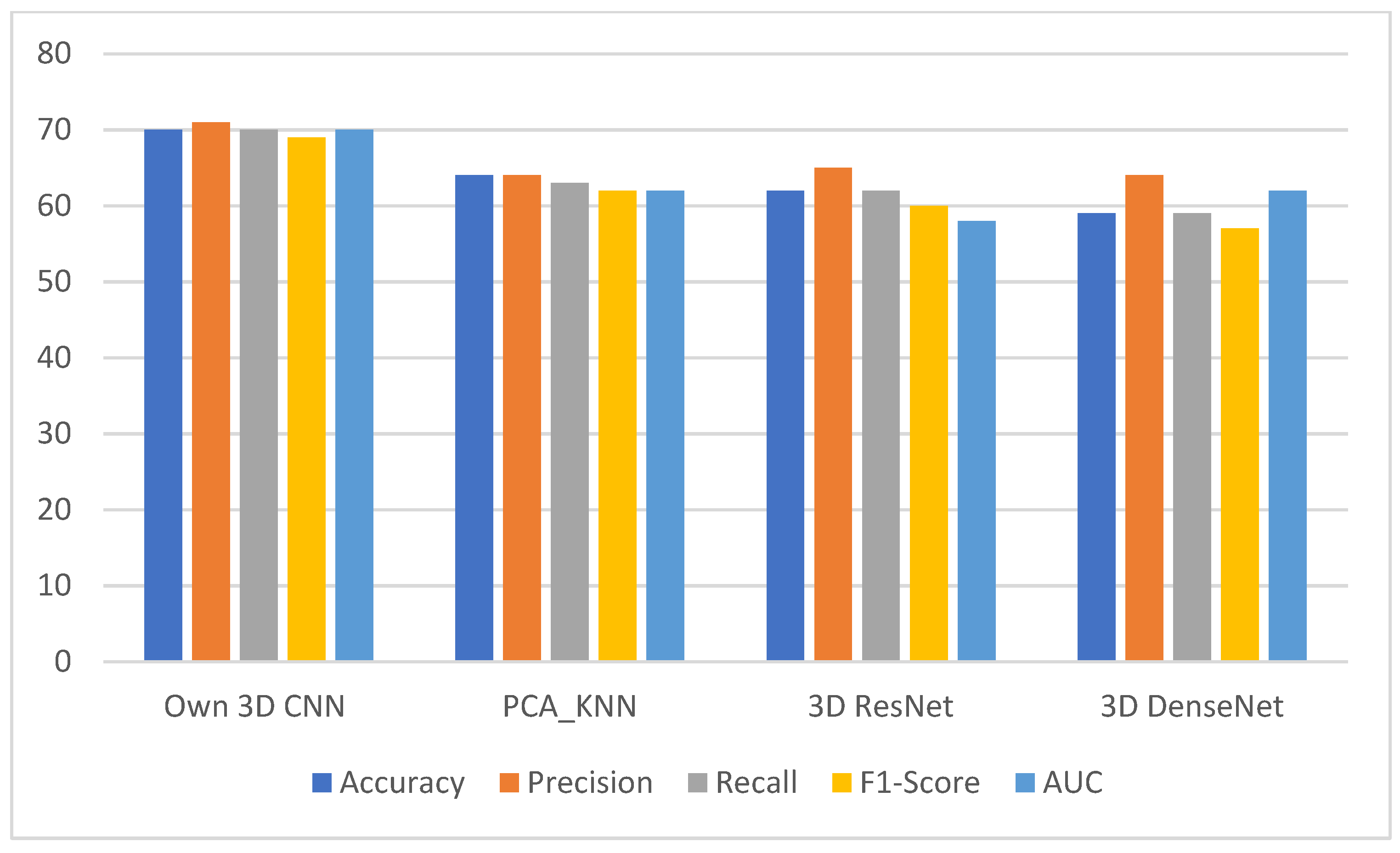
| Deep Learning Models | Accuracy | Precision | Sensitivity | F1-Score | AUC |
|---|---|---|---|---|---|
| Own 3D Net | 0.70 ± 0.02 | 0.71 ± 0.02 | 0.70 ± 0.02 | 0.69 ± 0.01 | 0.70 ± 0.04 |
| 3D DenseNet | 0.59 ± 0.05 | 0.64 ± 0.07 | 0.59 ± 0.05 | 0.57 ± 0.06 | 0.58 ± 0.13 |
| SEResNet50 | 0.62 ± 0.04 | 0.65 ± 0.07 | 0.62 ± 0.05 | 0.60 ± 0.04 | 0.62 ± 0.06 |
Publisher’s Note: MDPI stays neutral with regard to jurisdictional claims in published maps and institutional affiliations. |
© 2022 by the authors. Licensee MDPI, Basel, Switzerland. This article is an open access article distributed under the terms and conditions of the Creative Commons Attribution (CC BY) license (https://creativecommons.org/licenses/by/4.0/).
Share and Cite
Lisson, C.S.; Lisson, C.G.; Mezger, M.F.; Wolf, D.; Schmidt, S.A.; Thaiss, W.M.; Tausch, E.; Beer, A.J.; Stilgenbauer, S.; Beer, M.; et al. Deep Neural Networks and Machine Learning Radiomics Modelling for Prediction of Relapse in Mantle Cell Lymphoma. Cancers 2022, 14, 2008. https://doi.org/10.3390/cancers14082008
Lisson CS, Lisson CG, Mezger MF, Wolf D, Schmidt SA, Thaiss WM, Tausch E, Beer AJ, Stilgenbauer S, Beer M, et al. Deep Neural Networks and Machine Learning Radiomics Modelling for Prediction of Relapse in Mantle Cell Lymphoma. Cancers. 2022; 14(8):2008. https://doi.org/10.3390/cancers14082008
Chicago/Turabian StyleLisson, Catharina Silvia, Christoph Gerhard Lisson, Marc Fabian Mezger, Daniel Wolf, Stefan Andreas Schmidt, Wolfgang M. Thaiss, Eugen Tausch, Ambros J. Beer, Stephan Stilgenbauer, Meinrad Beer, and et al. 2022. "Deep Neural Networks and Machine Learning Radiomics Modelling for Prediction of Relapse in Mantle Cell Lymphoma" Cancers 14, no. 8: 2008. https://doi.org/10.3390/cancers14082008