1. Introduction
Adenoid cystic carcinomas (AdCys) are a rare and heterogenous subgroup of head and neck carcinomas. The combination of rare occurrence and heterogeneity even between two samples of the same tumor subtype makes histological differentiation from other types of head and neck cancers challenging [
1].
Previous studies have shown different levels of protein expressions in different types of salivary gland carcinomas (SGC) and MALDI imaging has successfully been used to confirm those results [
2,
3].
As a label-free imaging technique, MALDI imaging allows for the spatially resolved measurement of biomolecules in thin tissue sections. It has been demonstrated to be a useful tool for cancer research for the classification of different tumor species and the discovery of potential tumor marker proteins [
4,
5]
In combination with modern data analysis pipelines, MALDI imaging can be used for binary tumor classification as shown in [
6,
7,
8]. Recent results attained with more advanced machine learning show the applicability of MALDI imaging for the histologically challenging subtyping of different epithelial ovarian cancers [
9].
One of the most successful modern machine learning approaches is deep learning [
10]. Deep learning describes a class of artificial neural networks with multiple hidden layers that are used to solve a multitude of problems ranging from scene recognition for self-driving cars to medical applications such as tumor classification and segmentation in magnetic resonance imaging [
11,
12,
13]. A detailed overview of deep learning in medical imaging is given in [
14]. The type of artificial neural networks most commonly used in medical image and signal processing tasks is convolutional neural networks (CNNs) [
15]. With the increasing amount of labelled data available, this type of network has been used to achieve state-of-the-art performance in numerous tasks, such as image classification, speech recognition, and scene labeling [
16]. In some medical tasks, such as the detection of breast cancer metastasis, CNN-based machine learning approaches already outperform human experts [
17], [
18] and show promising results in the classification of skin diseases [
19].
With deep neural networks being used for critical decision-making in fields such as the aforementioned self-driving vehicles and tumor detection, there is a new need for understanding and interpreting the results of such algorithms. In recent years this goal has been worked toward by research in the field of explainable artificial intelligence (XAI) [
20].
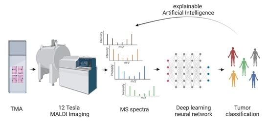
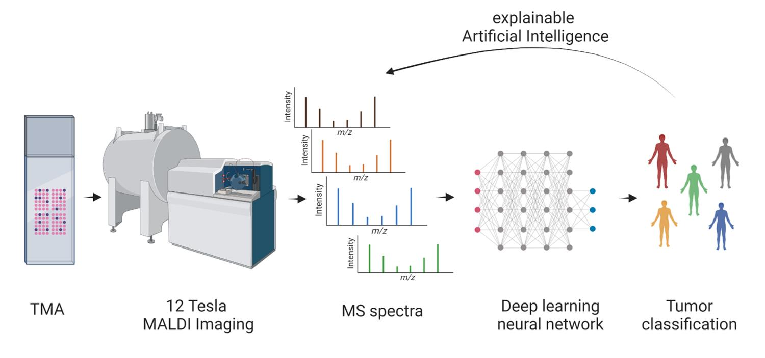
With this study, we aim to show that high mass resolution MALDI imaging supplemented with deep learning can be used to address the need to differentiate AdCys, which arise in the salivary gland from other types of SGCs. Additionally, we employ methods of explainable AI to identify masses which are significant for the detection of AdCys and match them to possible proteins. The spatially resolved nature of MALDI imaging allows us to compare the mass distributions with other histological methods.
To our knowledge, this approach has for the first time succeeded in performing an automated deep-learning-based classification of AdCys in comparison to other SGC subtypes. Since our analysis is based on MALDI-imaging and therefore includes a spatial component, we were able to analyze our results using methods of XAI and match them with histopathological insights.
2. Materials and Methods
2.1. TMA Preparation
Nineteen SGC samples (for clinicopathological data see
Table S1) from previously created tissue microarrays (TMAs) were included in the study. Samples were selected and reviewed by two pathologists with special expertise in the field as previously described (PMID: 34378164). Briefly, primary SGC FFPE blocks were retrieved from the archives of the Institute of Pathology at the University Hospital of Cologne. All diagnoses were critically reviewed using a panel of IHC and FISH tests (PMID: 34378164) before inclusion in the study. Four tissue cylinders with a diameter of 1.2 mm per case were included in the TMA. Additionally, we included tonsil and appendix samples from six healthy patients, which served as a technical control (
Table 1). Handling of patient material and data were in accordance with the ethical standards of the University of Cologne and the Helsinki Declaration of 1975 and its later amendments. Patients gave their written informed consent to participation.
2.2. Sample Preparation
TMA sections (6 µm) were mounted on indium tin oxide (ITO)-coated glass slides. Sample preparation was performed using SunTissuePrep (SunChrom, Friedrichsdorf, Germany). The protocol was consistent with previously published protocols [
21]. In brief, the subsequent steps were performed: deparaffinization, washing with xylene and ethanol, pH conditioning, and antigen retrieval. For on-tissue enzyme digestion, a trypsin solution of 2 µg/µL trypsin (Promega Gold) in 50 mM AMBIC buffer and 10% ACN was used. As the spraying device, the SunCollect System (SunChrom, Friedrichsdorf, Germany) was used. Digestion was performed with the SunDigest chamber (SunChrom, Friedrichsdorf, Germany) in basic mode. The matrix used for the experiments consisted of 10 mg/mL CHCA in 60% ACN and 0.2% TFA and was applied with the SunCollect.
2.3. MALDI Measurement
A dual source ESI/MALDI-FT-ICR mass spectrometer equipped with a dynamically harmonized analyzer cell (solariX XR, Bruker Daltonics Inc., Billerica, MA, USA) and a 12 T refrigerated actively shielded superconducting magnet (Bruker Biospin, Wissembourg, France) instrument was used for MALDI imaging. The instrument was operated in positive ionization, broadband mode (mass range 590–4000 m/z) with a 1 MW time domain (FID length: 1.677 s; mass resolution at m/z 1047: ~175,000). The measurement method was linearly calibrated with the Peptide Mix II (Bruker Daltonics) between 700 and 3200 Da (rms: 0.188 ppm, n = 8). The laser settings were optimized for spectral quality and peak magnitude (minimum focus, 9% laser power, 50 shots @ 2 kHz). MALDI imaging data were acquired using FlexImaging version 5.0 and ftmsControl version 2.3.0 (Bruker Daltonics) with a raster size of 50 µm.
2.4. Data Preprocessing
Using the SCiLS Lab Software (Bruker Daltonik, Bremen, Germany) we re-binned the individual spectra into equidistant 0.3 mDa bins and a mass range of 590 m/z–2000 m/z, which led to 217,984 data points per pixel. We performed no baseline removal or global normalization but normalized the intensities for each pixel to a range between 0 and 1.
With the co-registered microscopy images, we excluded all pixels that were part of a core but contained no tissue.
We also used the SCiLS Lab Software to find the 500 peaks best correlated with the highest pure matrix peak and created a dataset where all values in the range of 0.02 Da of these peaks were set to zero.
2.5. Deep-Learning-Based Classification
For the deep-learning task of tumor subtyping we treated each individual spectrum which corresponded to one measured spot as independent measurements with a single label. As described by [
22], these individual spectra possess similarities to images and can be processed using many of the same techniques proposed for image classification tasks.
Spectra are also similar to time-series data. Convolutional neural networks excel at solving practical problems on both types of datasets [
10].
We evaluated multiple different neural network architectures, including multiple combinations of fully connected and convolutional layers paired with pooling layers and leaky rectified linear units [
23] as activation function. All networks were implemented in Pytorch [
24] and the training was performed using the Adam optimizer at a learning rate of 0.001. All calculations were performed on a single Nvidia GeForce RTX 2080 Ti.
We evaluated all network architectures using 5-fold -cross-validation with random splits that aimed to preserve the ratio between the eight classes.
2.6. Deep Lift
DeepLift is one method of interpreting the results of a deep neural network, which allow for scoring the negative and positive contributions of each input feature to the predictions of a specific label. For a more detailed explanation we refer to the original work [
25]. We applied this method to our classification model to identify potential discriminative masses for each tumor subtype. We calculated the 10 input features with the highest positive contribution for each class.
2.7. Clustering with densMAP
To visualize the results of the DeepLift analysis, we performed a nonlinear supervised dimensionality reduction using densMAP [
26]. This method allowed us to visualize the high dimensional data points in our dataset. It is based on uniform manifold approximation and projection (UMAP) [
27] but learns to preserve and takes into account local density in the input space. As features we used the masses calculated in 2.6, and reduced the dimensionality to 2.
2.8. Comparison with Microscopy Images and Histological Assessment
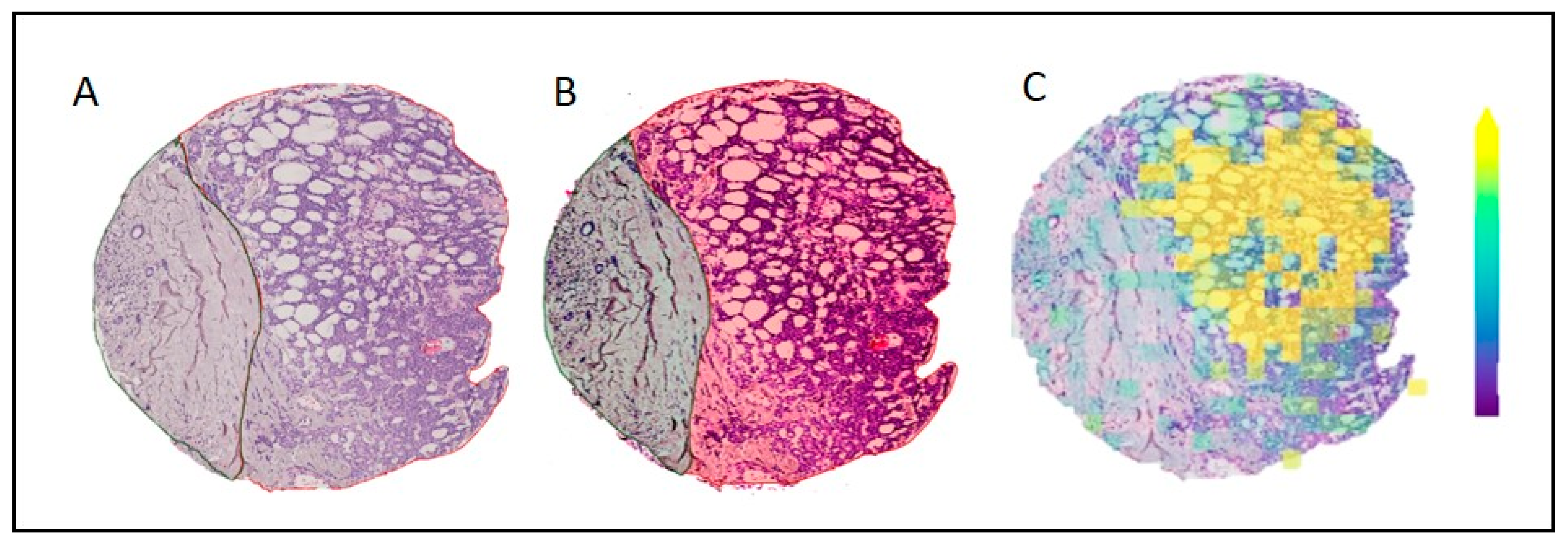
Finally, we visualized the distribution of the most significant predicted masses for the class AdCy. Using the SCiLS Lab Software, we overlaid this distribution onto a microscopy image of a core that contained AdCy tissue as well as healthy connective tissue. This allowed us to understand if the algorithm picked tumor-specific features or based its assessment on other characteristics of the sample.
3. Results
3.1. Network Architecture
On a small subset of the data, we observed the best performance using a convolutional neural net with six convolutional layers, each followed by a max pooling layer, and a final fully connected layer. We used this network architecture for all following experiments.
3.2. Classification Results
The final per-class classification accuracy, averaged over all test sets, is presented in
Table 2. The highest per-class accuracy was achieved on the control spot, which contained no tissue and was therefore the most homogenous class. The per-class accuracy of all SGC subtypes ranged from 83% to 87%. The lowest accuracy was achieved on the class Anos, which consists of multiple different not-further- specified adenocarcinomas of the salivary gland and shows a high level of heterogeneity.
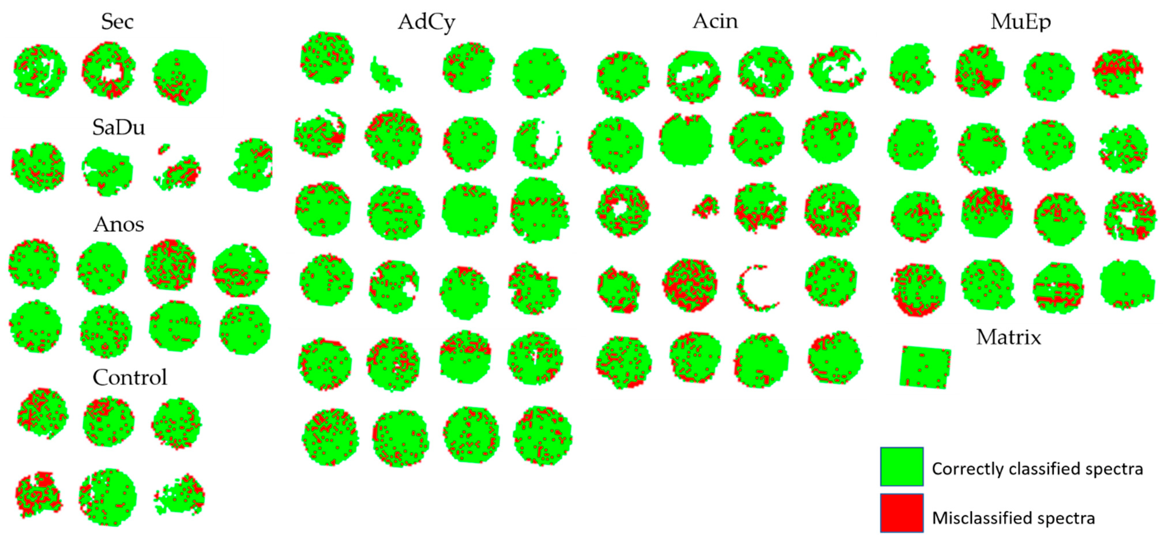
In
Figure 1, we visualize the classification results in the original pixel layout. We show correctly classified spectra represented as pixels in green and mark misclassifications in red. This visually demonstrates that the classification accuracy did not differ between different tumor subtypes or patients but that there were individual cores with higher percentages of misclassified spectra. We did not observe any correlation of the level of correctly classified spectra with histopathological features. We also evaluated the per-core accuracy by choosing the majority label for all pixels in one core. This resulted in 100% correct core-wise classification.
3.3. Predicted Masses
We analyzed the contribution of each mass to the prediction of each class using DeepLift. We then focused on the top ten contributions per class and further analyzed our dataset in regard to this list of masses. We filtered the resulting list of 80 masses (10 masses per class with 8 classes, see
Table S2) for duplicates and found that only 64 out of 80 masses appeared only in one tumor entity. The subset that contained duplicates can be matched to a measurement artifact. Therefore, we excluded this set from further analysis.
3.4. Clustering with densMAP
In
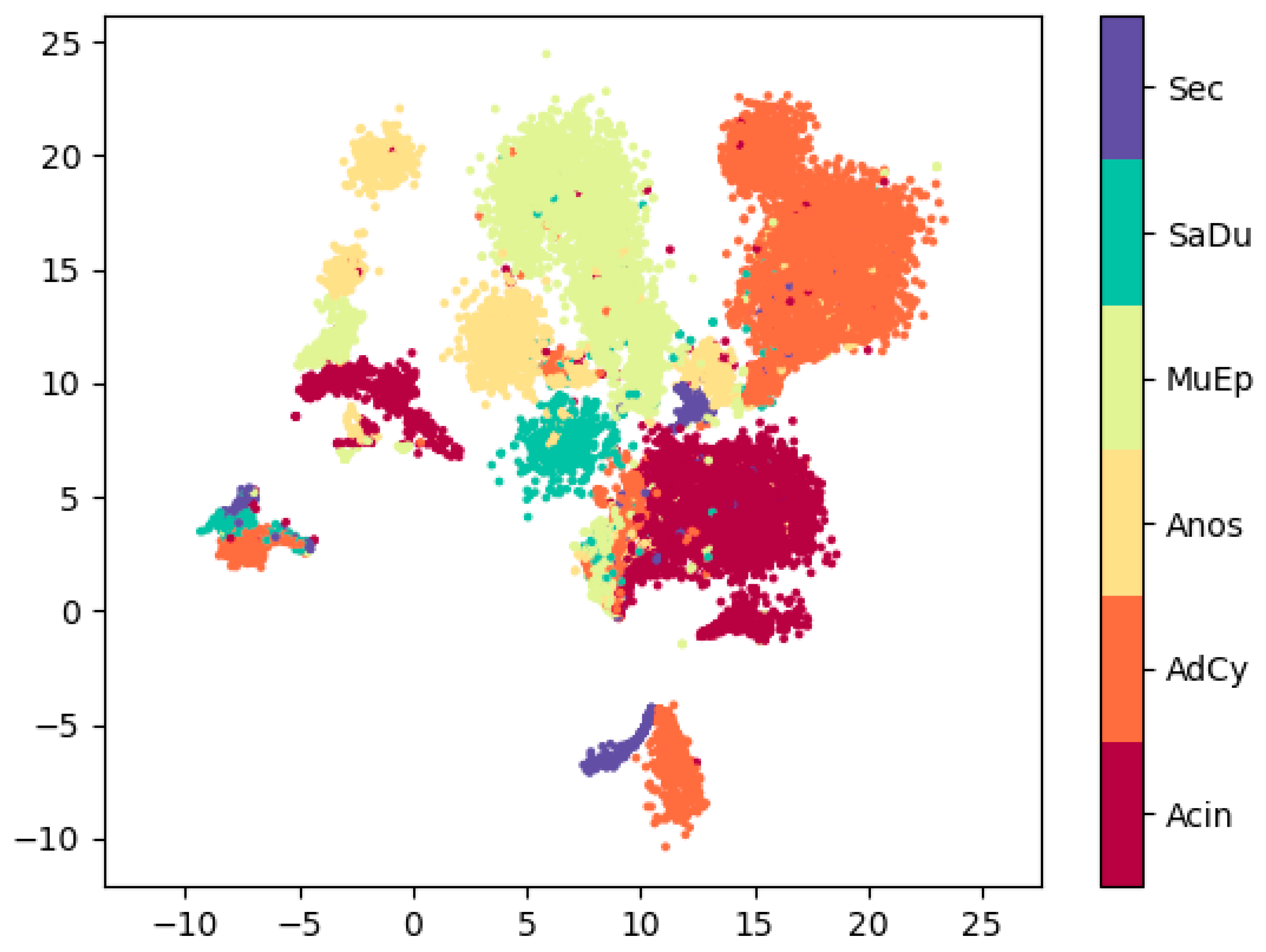
Figure 2 we plot the results of the dimensionality reduction using densMAP. The three SGC entities with the highest number of samples and therefore spectra (Acin, AdCy and MuEp) each show one large cluster containing the majority of samples. All three form additional smaller clusters. Further evaluation shows that these additional clusters all predominantly contain samples from one core. In the
Supplementary Materials we provide an interactive version of the above plot in which each point is mapped to its core. For the other SGC subtypes there is less of a clear clustering. This is expected for Anos, since these are a heterogenous group of SGCs. For the Sec, the class with the lowest number of samples, we observed strong inter-core differences. As a result, we get three distinct clusters, one for each Sec core.
3.5. Spatial Distribution and Comparison with Microscopic Imaging
We compared the distribution of the mass peak with the strongest positive contribution for the class AdCy to a microscopic view of a core that contained tumor tissue as well as healthy connective tissue (
Figure 3). This shows a high relative intensity in the tumor area and allows a differentiation between the two tissue types. With this result we show that the algorithm is picking up tumor-specific features.
4. Discussion
In this study we used high-resolution MALDI imaging data from a 12-Tesla instrument for a deep-learning approach. The aim was to provide a high classification accuracy on a challenging dataset consisting of six different SGC tumor subtypes, including AdCy, and healthy control samples.
Until now, high mass resolution MALDI imaging has been used to discriminate between different pathological regions in SGCs [
28] but not to differentiate between different subtypes of SGCs. In a similar way, deep-learning approaches to high-resolution MALDI imaging are, to the best of our knowledge, limited to binary classification tasks on mouse models [
29], and had not been applied before to tumor subtyping of SGCs.
With the aid of deep learning, we achieved above 80 percent per pixel classification accuracy on all tumor subtypes and a perfect whole-TMA core classification.
To get the most benefit out of the high mass resolution, we further applied techniques of explainable AI. This allowed us to interpret the results and predict masses that are most significant in predicting AdCy and other SGC entities. In this study, we applied DeepLift to get a list of ten masses per class with the strongest positive influence on the correct classification. This provided a better understanding of the results from a black-box-like deep-learning algorithm. Even before using these results for further experiments, this led us to discover a measurement artifact which allowed us to exclude 16 masses from further data analysis.
Using the predicted masses as features for a nonlinear dimensionality reduction method (NLDR) provides an extra layer of interpretability to the otherwise opaque classification approach. NLDR methods such as UMAP are a useful tool to visualize high-dimensional data [
30]. We applied densMAP, an augmented version of UMAP which has shown to provide better clustering with regard to the local density of the samples in the original space. The resulting plot shows that the majority of the data points originate from the three most prevalent SGC subtypes in our dataset, forming one large cluster each. A closer inspection reveals that there are single data points of each class appearing in clusters predominantly belonging to another class. This is in line with the high but not perfect classification accuracy of our deep-learning model. By investigating the origin of data points forming the smaller clusters we found that they almost exclusively represented single cores (interactive
Figure S1).
In the final step of our analysis, we mapped the mass with the most significant positive contribution to the class AdCy to microscopic images and histopathological annotations. Specifically, we validated our results by analyzing the distribution of this mass on a core that contained AdCy and healthy connective tissue. Since our dataset was composed almost exclusively of tumor tissue, this core presents an edge case. The fact that we observed a distinct distribution only in the tumor tissue of the core validates our approach. Additionally, this allows us to confirm the applicability of our deep-learning algorithm in the presence of small amounts of label noise (we incorrectly labelled the healthy tissue in this core as AdCy). This is consistent with the literature on this topic [
31] and supports our core-wise labelling strategy.
While we were able to interpret our classification results and get significant masses for the prediction of different SGC subtypes, we could not reliably match those experimental finds to specific proteins. Further work needs to be done in this protein identification task. Currently available technical and algorithmical solutions and absent dedicated databases do not provide satisfactory and verifiable results in this regard.
In contrast to our approach in which we searched for the presence of masses, another option for further study lies in the identification of masses with significant negative predictive power for certain SGC subtypes.
Regarding the applicability to a clinical setting, a recently published work shows that machine learning algorithms trained on MALDI imaging measurement of TMAs can successfully be transferred to classification tasks on whole sections [
32]. While these results were obtained with lung cancer patients, it seems likely that these results hold true for the tissue types and classification tasks presented in our study, since the experimental setup shows strong similarities and in both studies the task is cancer subtyping.
5. Conclusions
We were able to show that high mass resolution MALDI imaging in combination with deep learning can be used for tumor subtyping in SGCs. With methods of explainable AI and data visualization strategies based on nonlinear dimensionality reduction, we gained additional insights, for example into the homogeneity of the AdCy proteome among different patients. Additionally we were able to provide an intuitive understanding of deep-learning results by visualization of tumor-specific features combined with histopathological images. These allow us to verify the plausibility of our results and propose specific masses as a basis for further research into marker identification. Given the likely transferability of our TMA-based results, we see the potential for MALDI imaging as an additional diagnostic tool for the demanding task of SGC subtyping on the one hand and a general approach for other cancer entities on the other. To reach this goal, the following points have to be addressed: First, results should be evaluated in a larger independent tumor cohort. Secondly, the “black box” of deep learning can be further opened by methods of explainable AI for a better understanding of carcinogenesis, and in the long run enable better diagnostic and treatment regimes for cancers.
Supplementary Materials
The following supporting information can be downloaded at:
https://www.mdpi.com/article/10.3390/cancers14174342/s1, Table S1: Clinicopathological data; Table S2: Most significant masses for each tumor subclass; Interactive Figure S1: Interactive dense map clustering viewable in web browser, created using [
33].
Author Contributions
Conceptualization, O.G.-L., F.v.E. and F.H.; methodology, D.P. (David Pertzborn), C.A., G.E., O.G.-L., O.J.L., J.K., D.P. (Daniela Pelzel) and F.H.; software, D.P. (David Pertzborn); writing—original draft preparation, D.P. (David Pertzborn), F.v.E. and F.H.; writing—review and editing, F.v.E. and F.H.; supervision, F.v.E. and F.H. All authors have read and agreed to the published version of the manuscript.
Funding
This research was funded by the Carl Zeiss Foundation and CRIMSON-Coherent Raman Imaging for the molecular study of origin of diseases (EU Horizon 2020-ICT, grant number 101016923).
Institutional Review Board Statement
The study was conducted in accordance with the Declaration of Helsinki and approved by the Ethics Committee of the University of Cologne (protocol number 20-1588_1; date 6 May 2021).
Informed Consent Statement
Informed consent was obtained from all subjects involved in the study.
Data Availability Statement
The original data presented in the study are included in the article. Further inquiries can be directed to the corresponding author.
Conflicts of Interest
The authors declare no conflict of interest.
References
- Lorini, L.; Ardighieri, L.; Bozzola, A.; Romani, C.; Bignotti, E.; Buglione, M.; Guerini, A.; Lombardi, D.; Deganello, A.; Tomasoni, M.; et al. Prognosis and management of recurrent and/or metastatic head and neck adenoid cystic carcinoma. Oral Oncol. 2021, 115, 105213. [Google Scholar] [CrossRef] [PubMed]
- Wolber, P.; Nachtsheim, L.; Hoffmann, F.; Klußmann, J.P.; Meyer, M.; von Eggeling, F.; Guntinas-Lichius, O.; Quaas, A.; Arolt, C. Trophoblast cell surface antigen 2 (Trop-2) protein is highly expressed in salivary gland carcinomas and represents a potential therapeutic target. Head Neck Pathol. 2021, 15, 1147–1155. [Google Scholar] [CrossRef] [PubMed]
- Mayer, M.; Nachtsheim, L.; Hoffmann, F.; von Eggeling, F.; Guntinas-Lichius, O.; Prinz, J.; Klußmann, J.P.; Quaas, A.; Arolt, C.; Wolber, P. CD138 Is Expressed in Different Entities of Salivary Gland Cancer and Their Lymph Node Metastases and Therefore Represents a Potential Therapeutic Target. Int. J. Mol. Sci. 2022, 23, 9037. [Google Scholar] [CrossRef] [PubMed]
- Hoffmann, F.; Umbreit, C.; Krüger, T.; Pelzel, D.; Ernst, G.; Kniemeyer, O.; Guntinas-Lichius, O.; Berndt, A.; von Eggeling, F. Identification of proteomic markers in head and neck cancer using maldi–ms imaging, lc–ms/ms, and immunohistochemistry. Proteom. Clin. Appl. 2019, 13, 1700173. [Google Scholar] [CrossRef]
- Meding, S.; Nitsche, U.; Balluff, B.; Elsner, M.; Rauser, S.; Schöne, C.; Nipp, M.; Maak, M.; Feith, M.; Ebert, M.P.; et al. Tumor classification of six common cancer types based on proteomic profiling by MALDI imaging. J. Proteome Res. 2012, 11, 1996–2003. [Google Scholar] [CrossRef] [PubMed]
- Casadonte, R.; Kriegsmann, M.; Kriegsmann, K.; Hauk, I.; Meliß, R.; Müller, C.; Kriegsmann, J. Imaging mass spectrometry-based proteomic analysis to differentiate melanocytic nevi and malignant melanoma. Cancers 2021, 13, 3197. [Google Scholar] [CrossRef]
- Kriegsmann, M.; Casadonte, R.; Kriegsmann, J.; Dienemann, H.; Schirmacher, P.; Kobarg, J.H.; Schwamborn, K.; Stenzinger, A.; Warth, A.; Weichert, W. Reliable Entity Subtyping in Non-small Cell Lung Cancer by Matrix-assisted Laser Desorption/Ionization Imaging Mass Spectrometry on Formalin-fixed Paraffin-embedded Tissue Specimens. Mol. Cell. Proteom. 2016, 15, 3081–3089. [Google Scholar] [CrossRef]
- Kriegsmann, M.; Casadonte, R.; Maurer, N.; Stoehr, C.; Erlmeier, F.; Moch, H.; Junker, K.; Zgorzelski, C.; Weichert, W.; Schwamborn, K.; et al. Mass spectrometry imaging differentiates chromophobe renal cell carcinoma and renal oncocytoma with high accuracy. J. Cancer 2020, 11, 6081–6089. [Google Scholar] [CrossRef]
- Klein, O.; Kanter, F.; Kulbe, H.; Jank, P.; Denkert, C.; Nebrich, G.; Schmitt, W.D.; Wu, Z.; Kunze, C.A.; Sehouli, J.; et al. MALDI-imaging for classification of epithelial ovarian cancer histotypes from a tissue microarray using machine learning methods. Proteom. Clin. Appl. 2019, 13, 1700181. [Google Scholar] [CrossRef]
- Goodfellow, I.; Bengio, Y.; Courville, A. Deep Learning; MIT Press: Cambridge, MA, USA, 2016. [Google Scholar]
- Chen, L.; Zhan, W.; Tian, W.; He, Y.; Zou, Q. Deep integration: A multi-label architecture for road scene recognition. IEEE Trans. Image Process. 2019, 28, 4883–4898. [Google Scholar] [CrossRef]
- Khan, M.A.; Ashraf, I.; Alhaisoni, M.; Damaševičius, R.; Scherer, R.; Rehman, A.; Bukhari, S.A.C. Multimodal brain tumor classification using deep learning and robust feature selection: A machine learning application for radiologists. Diagnostics 2020, 10, 565. [Google Scholar] [CrossRef] [PubMed]
- Naser, M.A.; Deen, M.J. Brain tumor segmentation and grading of lower-grade glioma using deep learning in MRI images. Comput. Biol. Med. 2020, 121, 103758. [Google Scholar] [CrossRef] [PubMed]
- Zhou, S.K.; Greenspan, H.; Davatzikos, C.; Duncan, J.S.; Van Ginneken, B.; Madabhushi, A.; Prince, J.L.; Rueckert, D.; Summers, R.M. A review of deep learning in medical imaging: Imaging traits, technology trends, case studies with progress highlights, and future promises. Proc. IEEE 2021, 109, 820–838. [Google Scholar] [CrossRef]
- Sarvamangala, D.; Kulkarni, R.V. Convolutional neural networks in medical image understanding: A survey. Evol. Intell. 2021, 15, 1–22. [Google Scholar] [CrossRef]
- Gu, J.; Wang, Z.; Kuen, J.; Ma, L.; Shahroudy, A.; Shuai, B.; Liu, T.; Wang, X.; Wang, G.; Cai, J.; et al. Recent advances in convolutional neural networks. Pattern Recognit. 2018, 77, 354–377. [Google Scholar] [CrossRef]
- Liu, Y.; Gadepalli, K.; Norouzi, M.; Dahl, G.E.; Kohlberger, T.; Boyko, A.; Venugopalan, S.; Timofeev, A.; Nelson, P.Q.; Corrado, G.S.; et al. Detecting cancer metastases on gigapixel pathology images. arXiv 2017, arXiv:1703.02442. [Google Scholar]
- Vulli, A.; Srinivasu, P.N.; Sashank, M.S.K.; Shafi, J.; Choi, J.; Ijaz, M.F. Fine-Tuned DenseNet-169 for Breast Cancer Metastasis Prediction Using FastAI and 1-Cycle Policy. Sensors 2022, 22, 2988. [Google Scholar] [CrossRef]
- Srinivasu, P.N.; SivaSai, J.G.; Ijaz, M.F.; Bhoi, A.K.; Kim, W.; Kang, J.J. Classification of skin disease using deep learning neural networks with MobileNet V2 and LSTM. Sensors 2021, 21, 2852. [Google Scholar] [CrossRef]
- Das, A.; Rad, P. Opportunities and challenges in explainable artificial intelligence (xai): A survey. arXiv 2020, arXiv:2006.11371. [Google Scholar]
- Arolt, C.; Meyer, M.; Hoffmann, F.; Wagener-Ryczek, S.; Schwarz, D.; Nachtsheim, L.; Beutner, D.; Odenthal, M.; Guntinas-Lichius, O.; Buettner, R.; et al. Expression profiling of extracellular matrix genes reveals global and entity-specific characteristics in adenoid cystic, mucoepidermoid and salivary duct carcinomas. Cancers 2020, 12, 2466. [Google Scholar] [CrossRef]
- Behrmann, J.; Etmann, C.; Boskamp, T.; Casadonte, R.; Kriegsmann, J.; Maass, P. Deep learning for tumor classification in imaging mass spectrometry. Bioinformatics 2018, 34, 1215–1223. [Google Scholar] [CrossRef] [PubMed]
- Maas, A.L.; Hannun, A.Y.; Ng, A.Y. Rectifier nonlinearities improve neural network acoustic models. In Proceedings of the 30 th International Conference on Machine Learning, Atlanta, GA, USA, 16–21 June 2013. [Google Scholar]
- Paszke, A.; Gross, S.; Massa, F.; Lerer, A.; Bradbury, J.; Chanan, G.; Killeen, T.; Lin, Z.; Gimelshein, N.; Antiga, L. Pytorch: An imperative style, high-performance deep learning library. Adv. Neural Inf. Process. Syst. 2019, 32, 1–12. [Google Scholar]
- Shrikumar, A.; Greenside, P.; Kundaje, A. Learning important features through propagating activation differences. In Proceedings of the 34th International Conference on Machine Learning, Sydney, Australia, 6–11 August 2017. [Google Scholar]
- Narayan, A.; Berger, B.; Cho, H. Assessing single-cell transcriptomic variability through density-preserving data visualization. Nat. Biotechnol. 2021, 39, 765–774. [Google Scholar] [CrossRef] [PubMed]
- McInnes, L.; Healy, J.; Melville, J. Umap: Uniform manifold approximation and projection for dimension reduction. arXiv 2018, arXiv:1802.03426. [Google Scholar]
- Sommella, E.; Salviati, E.; Caponigro, V.; Grimaldi, M.; Musella, S.; Bertamino, A.; Cacace, L.; Palladino, R.; Di Mauro, G.; Marini, F.; et al. MALDI Mass Spectrometry Imaging highlights specific metabolome and lipidome profiles in salivary gland tumor tissues. Metabolites 2022, 12, 530. [Google Scholar] [CrossRef]
- Abdelmoula, W.M.; Stopka, S.A.; Randall, E.C.; Regan, M.; Agar, J.N.; Sarkaria, J.N.; Wells, W.M.; Kapur, T.; Agar, N.Y.R. massNet: Integrated processing and classification of spatially resolved mass spectrometry data using deep learning for rapid tumor delineation. Bioinformatics 2022, 38, 2015–2021. [Google Scholar] [CrossRef]
- Gardner, W.; Cutts, S.M.; Phillips, D.R.; Pigram, P.J. Understanding mass spectrometry images: Complexity to clarity with machine learning. Biopolymers 2021, 112, e23400. [Google Scholar] [CrossRef]
- Rolnick, D.; Veit, A.; Belongie, S.; Shavit, N. Deep learning is robust to massive label noise. arXiv 2017, arXiv:1705.10694. [Google Scholar]
- Janßen, C.; Boskamp, T.; Hauberg-Lotte, L.; Behrmann, J.; Deininger, S.; Kriegsmann, M.; Kriegsmann, K.; Steinbuß, G.; Winter, H.; Muley, T.; et al. Robust subtyping of non-small cell lung cancer whole sections through MALDI mass spectrometry imaging. Proteom. Clin. Appl. 2022, 16, 2100068. [Google Scholar] [CrossRef]
- Bokeh, D. Bokeh: Python Library for Interactive Visualization. 2018. Available online: http://www.bokeh.pydata.org (accessed on 14 July 2022).
| Publisher’s Note: MDPI stays neutral with regard to jurisdictional claims in published maps and institutional affiliations. |
© 2022 by the authors. Licensee MDPI, Basel, Switzerland. This article is an open access article distributed under the terms and conditions of the Creative Commons Attribution (CC BY) license (https://creativecommons.org/licenses/by/4.0/).

 ,
, 


