Article

A Novel Kalman Filter with State Constraint Approach for the Integration of Multiple Pedestrian Navigation Systems

1
Mobile Multi-Sensor Systems (MMSS) Research Group, Department of Geomatics Engineering, University of Calgary, 2500 University Drive NW, Calgary, AB T2N 1N4, Canada
2
College of Automation, Harbin Engineering University, Harbin 150001, China
3
GNSS Research Center, Wuhan University, 129 Luoyu Road, Wuhan 430079, China
*
Author to whom correspondence should be addressed.
Micromachines 2015, 6(7), 926-952; https://doi.org/10.3390/mi6070926
Submission received: 31 May 2015 / Revised: 8 July 2015 / Accepted: 9 July 2015 / Published: 16 July 2015
(This article belongs to the Special Issue Next Generation MEMS-Based Navigation—Systems and Applications)

Abstract

:
Numerous solutions/methods to solve the existing problems of pedestrian navigation/localization have been proposed in the last decade by both industrial and academic researchers. However, to date there are still major challenges for a single pedestrian navigation system (PNS) to operate continuously, robustly, and seamlessly in all indoor and outdoor environments. In this paper, a novel method for pedestrian navigation approach to fuse the information from two separate PNSs is proposed. When both systems are used at the same time by a specific user, a nonlinear inequality constraint between the two systems’ navigation estimates always exists. Through exploring this constraint information, a novel filtering technique named Kalman filter with state constraint is used to diminish the positioning errors of both systems. The proposed method was tested by fusing the navigation information from two different PNSs, one is the foot-mounted inertial navigation system (INS) mechanization-based system, the other PNS is a navigation device that is mounted on the user’s upper body, and adopting the pedestrian dead reckoning (PDR) mechanization for navigation update. Monte Carlo simulations and real field experiments show that the proposed method for the integration of multiple PNSs could improve each PNS’ navigation performance.

1. Introduction

The last few years have witnessed major progress in the development of pedestrian navigation systems (PNS). Common users of PNS mainly include the following:
  • First responders (e.g., emergency search and rescue personnel, police and military forces).
  • Recreational users (e.g., self-guided tourists, hikers, athletic trainers).
  • Other personnel (e.g., elderly people, visually impaired).
Micro-Electro-Mechanical System (MEMS) inertial sensors, miniature Global Navigation Satellite System (GNSS) receivers and wireless transmitters, Radio Frequency Identification Devices (RFID) chips, Bluetooth devices, and so on, are now widely used in PNS. MEMS inertial sensors, including accelerometers, gyroscopes, magnetometers, and barometers, are usually called self-contained sensors or inertial measurement units (IMU). Currently, most of the sensors mentioned above can be easily found in various consumer products, especially in the well-developed market for smart devices such as smart phones, smart watches, smart glasses, tablet computers, etc. Based on these sensors and devices, numerous researchers have been dedicated to PNS research. However, to date there are still major challenges for PNS to continuously, robustly, and seamlessly operate in all indoor and outdoor environments.

2. Literature Review and Problem Description

Most of the proposed techniques in recently published literature for PNS is concentrated in one of the following three groups:
  • Radio-navigation systems (GNSS, Cellular Networks).
  • Indoor infrastructure-based systems (RFID, Wi-Fi, Bluetooth, UWB (Ultra-wideband)).
  • MEMS sensor-based systems (inertial navigation system (INS), pedestrian dead reckoning (PDR)).

2.1. The Radio-Navigation Systems

GNSS is the primary source of information to provide the position of a PNS. However, GNSS can provide position information only under ideal conditions which require open environments (i.e., open space areas). In other words, the system works sporadically in urban and canopy areas due to signal blockage and attenuation [1]. Cellular network-based PNS were firstly described in [2], however, according to [3], in signal degraded areas such a system could suffer from poor accuracy and very low vertical resolution. This is a serious problem as in some extreme applications (e.g., indoor rescue), the location of the user on specific floors or in specific rooms is of great importance [4].

2.2. The Indoor Infrastructure-Based Systems

Numerous solutions to pedestrian navigation in indoor environments have been suggested in related literature. One effective way to meet this requirement is to use a RFID-based system [5]. In such an operation, the RFID tags should be installed beforehand at known locations; also, a device containing a RFID reader and an antenna should be carried by the user. When the user passes by a tag, the reader could then retrieve its location. However, such service is not always useful and applicable when a seamless location over large areas is required. Similarly, the Wi-Fi-, Bluetooth-, and UWB-based navigation methods could also provide efficient indoor navigation services [6]. However, the main reason for not always employing these methods for PNS is the obvious requirement of building dependent infrastructures.

2.3. The Micro-Electro-Mechanical System (MEMS) Sensor Based Systems

For MEMS sensor-based systems, due to the fact that MEMS sensors still have high noise ratio, the use of unaided Inertial Navigation System (INS) mechanization for PNS is very limited [7]. Considering the unique features of human walking steps, an effective approach to restrict the INS derived navigation errors is to mount the MEMS sensors on a foot of a user [8]. In such a mode of operation, when stance phases of the foot are periodically detected, the Zero Velocity Update (ZUPT) technique will be triggered to estimate and correct the INS navigation solution errors, as well as the inertial sensors’ inherent biases using a Kalman Filter (KF). Although the INS/ZUPT method could sometimes produce a relatively good navigation solution, however, due to the low observability of the heading error from the ZUPT, as well as the relatively large deterministic and random biases of the MEMS inertial sensors [9], and in cases of running scenarios, zero velocity intervals cannot be easily detected; thus, the deviations of navigation solutions continue to grow with time.
The other MEMS sensor-based approach is the Pedestrian Dead Reckoning (PDR) mechanization which also exploits the kinematics of human walking [10,11]. The main idea of PDR mechanization is to use accelerometer measurements to detect the user’s walking steps, estimate step length and propagate the user’s position using a measured azimuth between every two consecutive steps [12]. To data, various methods of step detection and step length calculation have already reached practical levels of accuracy whether the user walks in low-speed or runs in high-speed; thus, only the long-term azimuth accuracy remains challenging [13,14,15]. Moreover, it is noteworthy that the misalignment of the MEMS IMU with respect to a user’s body needs to be known [16,17]. Therefore, the PDR-based PNS is better rigidly mounted on the user’s upper body (e.g., chest and waist) since the misalignment can be almost unchangeable [18]. In addition, the user’s upper body does not block the GNSS signals, and the integration of PDR with a GNSS receiver could provide a PNS with superior performance in comparison with either stand-alone GNSS receivers or PDRs. GNSS-derived positions are excellent external measurements for updating the PDR, thus improving the PDR’s long-term accuracy. Similarly, the PDR can provide precise position solutions for GNSS signal reacquisition after outages in a short period of time. Moreover, it is noteworthy that why we prefer to choose this PDR/GNSS approach for the upper body mounted PNS instead of the INS/GNSS approach is that during GNSS outage periods, the INS positional errors will typically drift as a function of the cubical time, due to gyro drift. For instance, during 5 min of GNSS outage, the position error of the INS (e.g., the MEMS IMU embedded in the Samsung Note 2) could diverge by hundreds of kilometers [19].

2.4. The Multiple Systems Integration

From the above literature review, we can conclude that there is no navigation technology that, on its own, can provide a reliable, robust, and infrastructure-free solution to the problem of positioning a pedestrian in all kinds of indoor environments. Only a navigation system that acts in cooperation with a multitude of navigation technologies with complementary properties has the potential to fully solve pedestrian navigation problems. Because navigation technologies with complementary properties are generally based upon different physical phenomena, the most favorable location of the different sub navigation systems on the body of the user also differs. For example, GNSS-/Wi-Fi-/Bluetooth-/UWB-based systems are all best mounted or held on the upper body of the user because then it is least likely that other body parts will block the external signals; for using the INS mechanization-based PNS, the IMU is best mounted on a foot of a user, since the foot could then periodically become stationary whenever the user walks or runs; meanwhile for PDR-based PNS, it is best mounted on the user’s upper body, so that the user’s body does not block the GNSS signals, as well, the misalignment of the IMU with respect to the user’s body can be kept almost unchangeable, so if all navigation systems are located on different points of the user’s body, they will track the position of different points of the user’s body. Hence, there is a question about how to combine and make full use of these navigation solutions at the same time to further improve the accuracies of each sub-system. Also, considering the fact that in safety-related applications, it is imprudent to depend on a single navigation technique. Consequently, the concept of combining complementary navigation systems should be accepted for commercial applications.
Several forms of architecture have been proposed for the integration of multiple systems based PNS. Brand and Phillips [20] introduced the use of two MEMS IMUs for PNS fastened to each foot. The relative position updates between them are used to further improve both systems’ navigation results. Their method set up a local radio frequency (RF) infrastructure which uses RF phase changes between a reference signal located in a waist pack and the one coming from a transmitter located on each boot. Finally, a series of foot-to-foot range measurements can be updated. A drawback of this method is the use of RF infrastructure which is not available in most consumer devices. Bancroft [21] also placed two IMUs placed on the feet with the centralized KF method. The relative time-varying distances between them were regarded as a constant, which means the errors between the real distance and the assumed constant were ignored. Skog et al. [22] derived an inequality constraint to accurately describe the relative time-varying distances between the two foot-mounted IMUs. In addition, different from the centralized KF approach, they first introduced the idea of the state constraint KF into this problem, and changed the dual IMUs’ information-fusing problem into a weighted least squares problem. Laverne et al. [23] have also experimented with utilizing dual foot-mounted IMUs. Extremely high navigation accuracy has been reported by them, where ultra-sonic ranging was performed between two high-end IMUs (HG1930, Honeywell, Phoenix, AZ, USA) with gyro bias drifts only a few degrees per hour). Also, they announced that foot-to-foot range improved the heading estimate dramatically. However, these high-end IMUs are too bulky and expensive for regular pedestrian use, but the results indicate that high accuracy could also be achieved in future mass-market systems when small MEMS IMUs have improved in accuracy. Zampella et al. [24] proposed a new indoor PNS prototype which fuses the navigation results of a UWB-based system and a foot INS/ZUPT system through a probability density function (PDF) truncation approach, which requires a lot of calculations to approximate the truncated PDF mean and covariance. Also, this method does not consider the UWB non-line-of-sight conditions, namely when there exists the UWB signal outages.
In this research, we investigate the integration of multiple PNSs with constraints between them and propose a novel information fusion architecture that can be used to further improve the navigation accuracies of each PNS. In our mode of operation, if multiple PNSs are used at the same time by a user, the relative positions between any two PNSs are not fixed. However, there should be an upper bound on how far apart the two PNSs can be, so that the navigation solutions of the two systems together can compose a combined navigation solution which will explore the maximum spatial separation information of the two systems. The fusion of the two systems’ navigation solutions can be regarded as a KF with a state constraint problem. This requires the modifications of the two systems’ error state KF to exploit this additional information in order to estimate the optimal navigation solutions based on the state constrained KF algorithm. This method was first proposed by Simon and Chia [25], which considers a linear system and measurements describing movement of a land-based vehicle.
The remainder of this paper is organized as follows: a brief description of the state constrained KF is provided in Section 3. The INS/ZUPT and PDR/GNSS systems are then respectively discussed in Section 4 and Section 5, followed by the state constrained KF approach on the combined PNSs in Section 6. In Section 7, the performance of the new approach is analyzed through both simulation and the operational field experiments.

3. State Constraint Kalman Filter (KF)

This section first provides a brief summary of the unconstrained KF state estimate. Then the state constrained KF is shown as well as the method to solve the constrained KF problem. Finally, the solutions to four different constraint scenarios are separately presented.

3.1. State Unconstrained KF

Assuming x is a random vector with the dimension n, and has a nonsingular covariance matrix, P . We say that x is with Gaussian distribution only if its probability density function (PDF), p ( x ) , satisfies:
p ( x ) = 1 ( 2 π ) n / 2 1 | P | 1 / 2 exp [ 1 2 ( x m ) T P 1 ( x m ) ]
in which m = E [ x ] , P = E [ ( x m ) ( x m ) T ] , E [ ] is the expectation operator. For the standard linear KF system model:
{ x k = F  x k - 1 + w k - 1 z k = H x k + v k
w k - 1 and vk are jointly Gaussian. When measurement z k is given, through the application of KF, we could get the optimal estimate, x ^ k , i.e., the minimum variance estimate. Referring [26], x ^ k is given by:
x ^ k = E [ x k | z k ] = m k + Pk x z ( P k z z ) 1 ( z k z ¯ k )
where m k = E [ xk ] , Pk x z is the covariance matrix of xk and z k , Pk z z is the covariance matrix of z k . As x ^ k is conditionally Gaussian given z k , so we say x ^ k and z k are jointly Gaussian. Similar to Equation (1), p ( x | z ) is the conditional PDF of x given z :
p ( x | z ) = 1 ( 2 π ) n / 2 1 | P | 1 / 2 exp [ 1 2 ( x x ^ ) T P 1 ( x x ^ ) ]
where P is the covariance matrix of the KF estimate, which can be calculated as:
P = P xx P x z ( P z z ) 1 P z x
and the KF estimate x ^ is the calculation of x that maximizes p ( x | z ) .

3.2. State Constrained KF

Assuming that the state x of the linear system model given Equation (2) satisfies the equality constraint:
Γ ( x ) = d
or the inequality constraint,
Γ ( x ) d
where Γ ( ) is a known linear or nonlinear operator for x , and d is a known vector. After normal KF process, if the state does not satisfy the above given constraints, we need to find a new state estimate, x ˜ .

3.3. Maximum Probability Algorithm

Obtaining the new constrained state can be solved through the maximum probability algorithm [25]. We know that the KF estimate is the value of x that maximizes p ( x | z ) in Equation (4). Similarly, the constrained state can be derived by calculating the new estimate, x ˜ , so that p ( x | z ) is further maximized and x ˜ satisfies the constraints. Maximizing p ( x | z ) is the same as maximizing its natural logarithm:
x ˜ = max x ˜  p ( x ˜ | z )    = max x ˜ {ln[ p ( x ˜ | z ) ] }    = max x ˜ { ( x ˜ x ^ ) T P 1 ( x ˜ x ^ ) 2 } ln { 1 ( 2 π ) n / 2 1 | P | 1 / 2 }    = min x ˜ [ ( x ˜ x ^ ) T P 1 ( x ˜ x ^ ) ]    = min x ˜ [ x ˜ T P 1 x ˜ 2 x ^ T P 1 x ˜ + x ^ T P 1 x ^ ]
in which x ^ is the KF state estimate, thus x ^ T P 1 x ^ is a known component before applying the constraint. The constrained estimate x ˜ can therefore be calculated using the following Equations (9) and (10):
x ˜ = min x ˜ [ x ˜ T P 1 x ˜ 2 x ^ T P 1 x ˜ ]
s . t .     Γ ( x ˜ ) = d    o r    Γ ( x ˜ ) d

3.4. The Solutions to the State Constrained KF

The constraints given in Equations (9) and (10) can be divided into four different scenarios. If the operator Γ ( ) is linear, namely, Γ ( x ˜ ) = κ x ˜ , we then have the linear equality constraint, κ x ˜ = d , or the linear inequality constraint, κ x d . Worth noting is that κ is a known constant r × n matrix with full rank r , and d is a known r × 1 vector, namely the number of rows in κ is the number of constraints. If κ is a square matrix, the state is fully constrained, but κ is not full rank which means we have redundant state constraints, at this time we need to remove the linearly dependent rows from κ until κ is full rank. Similarly, if Γ ( ) is a non-linear operator, we assume Γ ( x ˜ ) = η ( x ˜ ) , in which η ( x ˜ ) is the nonlinear expression of x ˜ . We then have the non-linear equality constraint, η ( x ˜ ) = d , or the nonlinear inequality constraint, η ( x ˜ ) d . The solutions to the four different state constrained KF scenarios are separately given as follows.

3.4.1. The State Linear Equality Constrained Solution

According to Equations (9) and (10), the problem we want to solve here can be written as:
x ˜ = min x ˜ [ x ˜ T P 1 x ˜ 2 x ^ T P 1 x ˜ ]
s . t .    κ  x ˜ = d
To get the solution x ˜ , we form the Lagrange function [25]:
L ( x ˜ ,  λ ) = x ˜ T P 1 x ˜ 2 x ^ T P 1 x ˜ + λ T ( 2 κ  x ˜ 2 d )
For the convenience of calculation, the constraint of Equation (12) was written as 2  κ  x ˜ = 2  d . The first order conditions for the minimum of Equation (11) are:
{ ( x ˜ , λ ) x ˜ = 2 P 1 ( x ˜ x ^ ) 2 κ T λ = 0 ( x ˜ , λ ) λ = κ x ˜ d = 0
Then the Equation (14) gives the following solutions ( λ , x ˜ ) :
{ λ = ( κ P κ T ) 1 ( κ x ^ d ) x ˜ = x ^ P κ T ( κ P κ T ) 1 ( κ x ^ d )
After we get the new constrained state, x ˜ , we also need to update the new state error covariance, P * . From Equation (15), we have:
x x ˜ = x x ^ + P κ T ( κ  p  κ T ) 1 [ κ x ^ d ( κ x d ) ]    = [ Ι P κ T ( κ  p  κ T ) 1 κ ] ( x x ^ )    = ( Ι μ ) ( x x ^ )
in which P  κ T ( κ P κ T ) 1  κ is denoted by μ , and x is the true state. Then the constrained new state error covariance, P * , can be expressed as:
P * = E ( x x ˜ ) ( x x ˜ ) T ]       = E { [ ( Ι μ ) ( x x ^ ) ] [ ( Ι μ ) ( x x ^ ) ] T }       = ( Ι μ ) P ( Ι μ ) T

3.4.2. The State Linear Inequality Constrained Solution

Assuming that the KF state satisfies the inequality constraint, the constrained state, x ˜ , can be derived as:
x ˜ = min x ˜ ( x ˜ T P 1 x ˜ 2 x ^ T P 1 x ˜ )
s . t .    κ  x ˜ d
The above problem is known as a Quadratic Programming (QP) of the mathematical optimization [27]. QP problems can be solved using the active set algorithm, which reduces the number of constraints to those which are active within the solution to the QP problem. The basic strategy of active set algorithm is that first we make an explicit estimate of the active set, and then take a step toward the solution using a simplified QP problem in which the constraints in this estimated active set are satisfied as equalities, a brief explanation to this algorithm can be seen in [27] (pp. 240–245). For instance, we take into consideration the Equations (18) and (19) as an example of the problem. Supposing we have s inequality constraints, q of the s inequality constraints are active at the solution of Equation (18), denoted by κ * . The q rows of κ that correspond to the active constraints, are denoted by d * , and the q components of d correspond to the active constraints. If the correct set of active constraints is known a priori then the solution to the problem given in Equations (18) and (19) is also the solution to the equality constraint problem:
x ˜ = min x ˜ ( x ˜ T P 1 x ˜ 2 x ^ T P 1 x ˜ )
s . t .     κ * x ˜ = d *
So it is demonstrated that the inequality constraint problem of Equations (18) and (19) is equivalent to the equality constraint problem only and if only we know the correct a priori active sets, at this time the solution-solving method given in Section 3.4.1 also applies to the state inequality constraint problem.

3.4.3. The State Non-Linear Equality Constrained Solution

The problem we want to solve at this time can be expressed as:
x ˜ = min x ˜ ( x ˜ T P 1 x ˜ 2 x ^ T P 1 x ˜ )
s . t .     η ( x ˜ ) = d
in which η ( x ˜ ) is the non-linear expression of x ˜ . We suppose that the linear model in Equation (2) has been estimated by the KF procedure, and yields an unconstrained estimate x ^ . Assuming that x ^ is “close” to the constrained estimate x ˜ , at this time the non-linear constraint problem can be linearized (Taylor’s expansion) around the current unconstrained state estimate, x ^ :
η ( x ˜ ) d = η ( x ^ ) + [ η ( x ^ ) ] T ( x ˜ x ^ ) + 1 2 ( x ˜ x ^ ) T η ( x ^ ) ( x ˜ x ^ ) + d
in which η ( x ^ ) and η ( x ^ ) denote the first and second partial derivatives of η ( x ) with respect to x , replacing x with x ^ . Neglecting the second-order and higher terms yields:
η ( x ^ ) x ˜ d η ( x ^ ) + [ η ( x ^ ) ] T x ^
The above equation is equivalent to the linear constraint κ ˜ x ˜ = d ˜ , in which:
κ ˜ = [ η ( x ^ ) ] T
d ˜ = d η ( x ^ ) + [ η ( x ^ ) ] T x ^
So the method presented in Section 3.4.1 can also be used to solve the nonlinear inequality constraint problem after the constraint is linearized.

3.4.4. The State Non-Linear Inequality Constrained Solution

The problem we want to solve is shown as:
x ˜ = min x ˜ ( x ˜ T P 1 x ˜ 2 x ^ T P 1 x ˜ )
s . t .     η ( x ^ ) d
Similar to Section 3.4.3, the non-linear constraint can first be linearized, then the problem will be changed into the linear inequality constraint problem. If the set of the active constraints was known a priori, then the linear inequality constraint will be equivalent to the equality constraint, and the method given in Section 3.4.1 is also applicable.

4. The Inertial Navigation System/Zero Velocity Update (INS/ZUPT) System

We fuse different PNSs to evaluate the state constrained KF algorithm. One PNS is a foot-mounted INS/ZUPT system, which operates in two parts: INS Mechanization to compute the position, velocity and attitude; and an EKF-based ZUPT is triggered to estimate and composite the navigation state errors.

4.1. INS Mechanization

The continuous model (differential equation) of INS mechanization can be given as follows [19,28]:
[ r ˙ n v ˙ n T ˙ b n ] = [ D 1 v n T b n f b 2 ( Ω i e n + Ω e n n ) + g n T b n ( Ω i b b Ω i n b ) ]
where the navigation frame, n, is the local-level frame (local North, East, and Down, i.e., N-E-D), rn = [ r x r y r z ] T is the INS derived position, v n = [ v x v y v z ] T denotes the velocity, and T b n is the transition matrix describing the body frame b relative to n frame, the attitude vector, ε (pitch, roll and heading), can be derived from T b n , f b denotes the accelerometer output, and ω b the angular velocity measured by the gyroscope. To get the navigation solution, we assume the sampling period of INS is Δ t , the non-linear function ξ denotes INS mechanization. At time step k, the navigation solution xk i n s = [ r k n v k n ε k ] T can be updated as:
xk i n s = ξ ( x k 1 , fk b , ω k b ) ,    x 0 i n s = [ i n i t i a l v a l u e ]
in which x 0 is the initial value of INS. More details about the discrete representation of INS mechanization can be found in [29,30].

4.2. INS Error Model

The INS error model used in this research is given in the following compact form [29]:
δ x ˙ i n s = [ D 1 δ v n N n ε ( 2 Ω i e n + Ω e n n ) δ v n + V n ( 2 δ ω i e n + δ ω e n n ) + δ g n Ω i n n ε δ ω i n n ] + G i n s w i n s
where the vector δ xk i n s = [ δ r k n δ v k n δ ε k ] T is the INS error state including error components of position, velocity and attitude. w i n s is the sensor noise vector, and G i n s is the noise distribution matrix. Equation (32) can be briefly represented by:
δ x ˙ i n s = F i n s δ x i n s + G i n s w i n s
The above equation is the first-order differentiation of the error state δ x i n s . A detailed expression of Equation (33) can be found in [29]. F i n s is the dynamic coefficient matrix which contains the INS error models for the position, velocity, and attitude. The discrete-time form of Equation (33) can be written as:
δ x k + 1 i n s = Φ k + 1 ,  k i n s δ xk i n s + Gk i n s w k i n s
where Φ k + 1 ,  k i n s is the discrete-time error state transition matrix from epoch k to k + 1.

4.3. INS Error Correction Using ZUPT

The discrete measurement model at time step k is expressed as:
δ z k i n s / z u pt = H k i n s / z u pt δ xk i n s + ν k i n s / z u pt
where δ z k i n s / z u pt is the measurement vector, which is the true velocity (zero velocity) of the system minus the velocity vector derived from the INS during the system’s static mode. ν k i n s / z u pt is the measurement noise matrix. The measurement matrix H k i n s / z u pt is:
H k i n s / z u pt = [ 0 3 × 3 I 3 × 3 0 3 × 3 ]
Every time the state errors δ x i n s are updated, these are applied to the INS navigation solution, then δ x i n s is reset, which means the error state prediction procedure is no longer required.
In this research, we have achieved good zero-velocity detection results using the detection method described in [31] and [32]. Their detection methods are checked through the magnitude of the acceleration, magnitude of gyroscope, and local acceleration variance. Several papers, including [33] and [34], etc., have also discussed zero-velocity detection methods in detail. Readers can refer to this literature for more information on the detection procedure.

5. The Pedestrian Dead Reckoning/Global Navigation Satellite System (PDR/GNSS) System

This section will presents the PDR/GNSS system prototype. The information on user’s travelled distance and heading given by PDR mechanization are merged with the GNSS-derived observations through standard KF.

5.1. PDR Mechanization

The PDR algorithm can be implemented in the following mechanization [35]:
{ E   k + 1 = E k + S k sin ( ψ k ) N   k + 1 = N k + S k cos ( ψ k )
in which Ek+1 is the PDR navigation estimation along local east at time step k + 1, Nk+1 is the PDR navigation estimation along local north at time step k + 1, Sk is the estimated pedestrian step length from time step k to k + 1, ψ k is the estimated pedestrian step heading at time step k. Worth noting is that the given PDR mechanization only represents a 2-dimension (2D) navigation scheme.

5.2. PDR Error Model

The complete discrete PDR error transition model is given as follows [36]:
{ δ E k + 1 = δ E k + S k cos ( ψ k ) ψ k + sin ( ψ k ) δ S k δ N k + 1 = δ N k S k sin ( ψ k ) δ ψ k + cos ( ψ k ) δ S k δ ψ k + 1 = δ ψ k + Δ t  δ b k δ S k + 1 = δ S k + ( w S ) k δ b k + 1 = ( 1 α Δ t ) δ b k + ( w b ) k
where δ E and δ N are respectively the eastern and northern position errors; δ ψ is the error on the heading induced by the Z (up) gyro bias error δ b , which is considered as the random process with zero mean, the correlation time T c = α - 1 and the driven noise w b ; the step length error δ S is considered as a white noise w S with the variance σ S 2 . Similar to the INS error model, then Equation (38) can be written as:
δ x k + 1 pdr = Φ k + 1 ,  k pdr δ xk pdr + Gk pdr w k pdr
where the vector δ x pdr = [ δ E δ N δ ψ δ S δ b ] T is the PDR error state vector. Then the transition matrix, Φ k + 1 ,  k pdr , from time step k to k + 1 can be written as:
Φ k + 1 ,  k pdr = [ 1 0 S k cos ( ψ k ) sin ( ψ k ) 0 0 1 S k sin ( ψ k ) cos ( ψ k ) 0 0 0 1 0 Δ t 0 0 0 1 0 0 0 0 0 ( 1 α Δ t ) ]

5.3. PDR Error State Correction Using GNSS

The measurement model has the following linear form:
δ z k pdr / gn s s = H k pdr / gn s s δ xk pdr + ν k pdr / gn s s
where the measurement noise vector, ν pdr / gn s s , is assumed to be a zero-mean white Gaussian noise process. The measurement matrix, H k pdr / gn s s , should have the form:
H k pdr / gn s s = [ I 3 × 3 0 3 × 2 ]
The measurement vector is:
δ z k pdr / gn s s = [ E k g n s s E k P d r N k g n s s N k P d r ψ k g n s s ψ k pdr ] T
in which E k gn s s is the GNSS-measured east position at time step k; Nk gn s s is the measured north position from the GNSS; ψ k gn s s is the GNSS heading. The common method to determine ψ k gn s s is the use of GNSS velocities, and is given by:
ψ k gn s s = arctan ( V k g n s s , E V k g n s s , n )
where Vk gn s s , E is the east GNSS-derived velocity at time step k, and Vk gn s s ,  n is the north GNSS velocity.

6. Information Fusion of Two Navigation Systems Using State Constraint KF

In this section, we first formulate the constraint between two PNSs’ navigation states, then derive the solution to the constraint problem by applying the method given in Section 3.

6.1. Constraint between Two Navigation Systems

Assuming that we have two PNSs: one is the INS/ZUPT system, the other one is the PDR/GNSS system. We denote the first two elements of INS/ZUPT system’s navigation state, X i n s = [ r n v n ε ] T , as X 1 = [ r x r y ] T , in which r x and r y are respectively the position solutions along the direction of local East and North. The first two states of PDR/GNSS system’s navigation state, X pdr = [ E N ψ S b ] T , is expressed as X 2 = [ E N ] T . We denote the combined navigation solution of the two PNSs as:
X = [ X i n s X p d r ] T
As depicted in Section 1, the INS/ZUPT system is mounted on a user’s foot, the PDR/GNSS system is held on the upper body of the user. During the navigation process, there is always a maximum horizontal distance between the two PNSs, namely:
| | X 1 X 2 | | 2 d 2
where d is a constant representing the maximum distance. For the convenience of the further matrix calculations, Equation (46) can be simplified by:
| | κ X | | 2 = ( κ  X ) T ( κ X ) d 2
in which matrix κ is expressed as:
κ = [ I 2 × 2 0 2 × 7 I 2 × 2 0 2 × 3 ]
The combined position solution X should always satisfy Equation (47), if not, when | | κ X | | 2 > d 2 , we should employ the state constraint KF to restrict X onto the space of Equation (47). So the constrained new estimate, X ˜ , can be calculated as:
X ˜ = min X ˜ ( X ˜ T P 1 X ˜ 2 X ^ T P 1 X ˜ )
s . t .     ( κ  X ˜ ) T ( κ X ˜ ) d 2
where P in Equation (49) is the covariance matrix of the combined position solution, X , which is obtained from the EKF-based INS. Worth noting is that for each navigation system, the position part of the navigation state covariance matrix is updated separately for each EKF. When the combined navigation state does not satisfy ( κ  X ) T ( κ X ) d 2 , the state constraint algorithm will be applied. At this time, the combined covariance matrix Cov for Equation (49) can then be expressed as:
P = [ P 9 × 9 i n s 0 9 × 5 0 5 × 9 P 5 × 5 p d r ]
in which P 9 × 9 i n s and P 5 × 5 pdr are the covariance matrices respectively representing the navigation error standard deviations of the INS/ZUPT system and PDR/GNSS system.

6.2. The Solution to the Constraint Problem

From Equation (50) we can see the given constraint is an in-equality problem, and both ( κ  X ) T ( κ X ) and d 2 can be regarded as the 1 × 1 matrices, so Equation (50) cannot be written in the form of several rows, which means there is only one constraint set. So the optimal solution X * (a feasible point of the constraint) to the problem given in Equation (50) should definitely satisfy the equality constraint:
( κ  X * ) T ( κ X * ) = d 2
such that the in-equality constraint, ( κ  X ) T ( κ X ) d 2 , is an active constraint of X * . Thus, the problem given in Equations (49) and (50) can be changed into:
X ˜ = min X ˜ ( X ˜ T P 1 X ˜ 2 X ^ T P 1 X ˜ )
s . t .     ( κ  X ˜ ) T ( κ X ˜ ) = d 2
Then the constraint in Equation (54) can be linearized (Taylor’s expansion) about the current unconstrained state estimate, X ^ . Neglecting the second-order and higher terms of the Taylor’s expansion, we have:
( 2 κ T  κ  X ^ ) T X * = d 2 ( κ  X ^ ) T ( κ X ^ ) + ( 2 κ T  κ  X ^ ) T X ^
The Equation (55) is equivalent to the linear constraint, κ ˜ X * = d ˜ , in which:
κ ˜ = ( 2 κ T  κ  X ^ ) T
d ˜ = d 2 ( κ  X ^ ) T ( κ X ^ ) + ( 2 κ T  κ  X ^ ) T X ^
So the solution to the problem in Equations (53) and (54) is given as:
X * = X ^ P κ ˜ T ( κ ˜ P  κ ˜ T ) 1 ( κ ˜ X ^ d ˜ )
According to Section 3.4.1, the new covariance of the constrained navigation solution, represented by P * , is updated as follows:
P * = ( Ι μ ) P ( Ι μ ) T
in which μ is expressed as:
μ = P κ ˜ T ( κ ˜ P  κ ˜ T ) 1 κ ˜
In terms of the system implementation, as well as theoretically compared to the existing techniques given in the literature review those also use spatial constraints, it can be seen from the above Equations (58) and (59) that our proposed method only requires slightly more computational effort than the unconstrained filter. That is all because our proposed approach is quite similar to the way of implementing an Extended Kalman filter (EKF), which relies on the linearization of the system and measurement equations. The linearization of the constraint is done beforehand, such that the implementation procedure of the constraint filter is as easy as substituting the KF-derived navigation state X ^ and state covariance P into Equations (58) and (59).
However, the constraint filter given in [21] requires much higher computational complexity because of the additional quadratic programming problem that needs to be solved. To get the solution to the constraint filter, first, the authors changed the quadratic problem into a Lagrange multiplier λ-based quadratic equation root-finding problem. A nonlinear polynomial function was then constructed, and to find the roots to the nonlinear polynomial function, one must resort to some numerical root finding methods, in [21], Newton’s method is used, then, based on the iteration of the Newton’s method, the Lagrange multiplier λ can be found, consequently the solution to the constraint filter can then be further resolved. For implementing such a constraint filter, the computational burden is mainly caused by the multiple iterative calculations to find a converged Lagrange multiplier λ.
Similarly, compared to the method given by Zampella et al. [24], their constraint filter adopts a probability density function (PDF) truncation approach, which requires a lot of calculations to approximate the truncated PDF mean and covariance. To be specific, their constraint filter uses a particle filter way to calculate the propagation of the mean and covariance of the propagated states of the constraint filter. Moreover, in the conclusion part of [24], the authors also address that it requires many calculation burdens to implement their constraint filter.

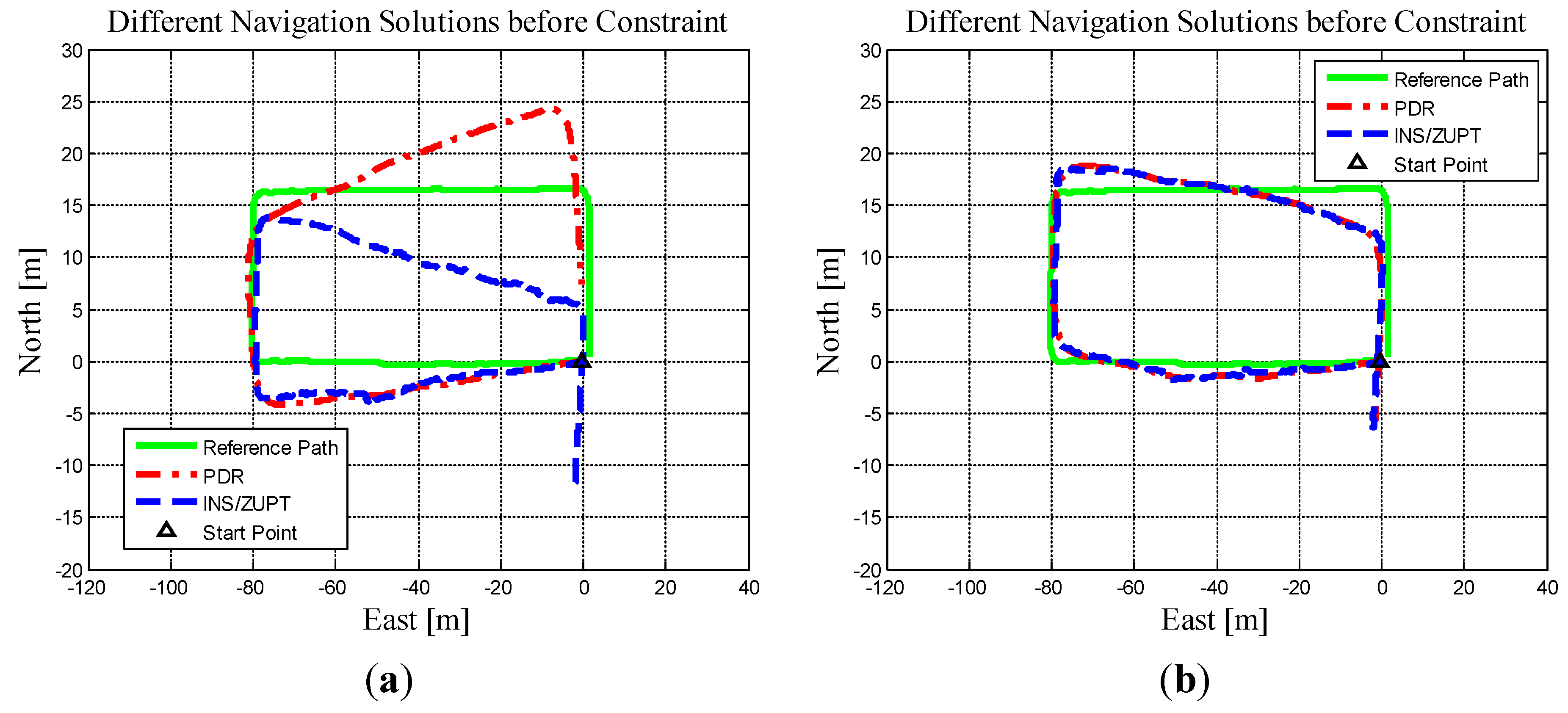
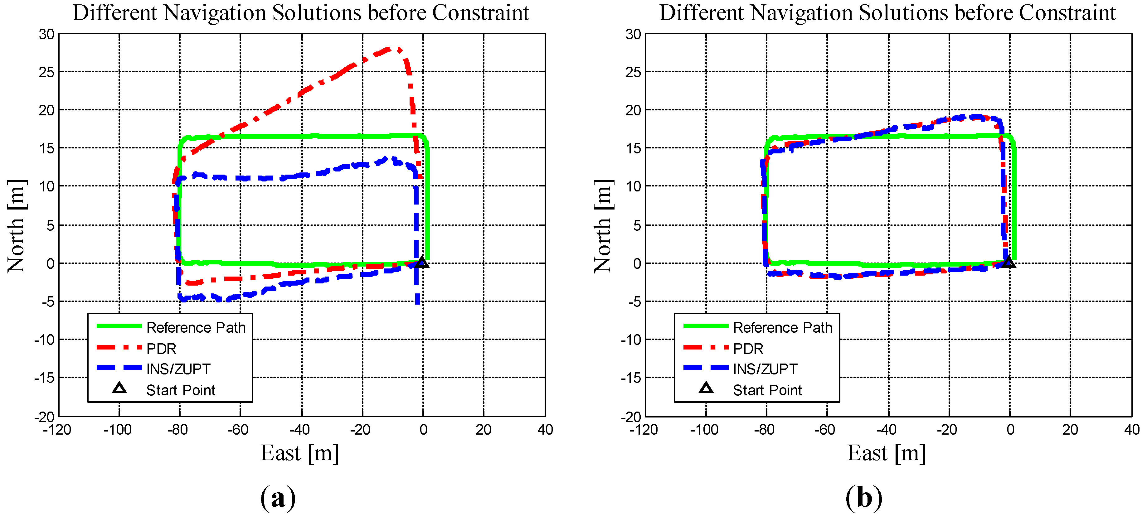
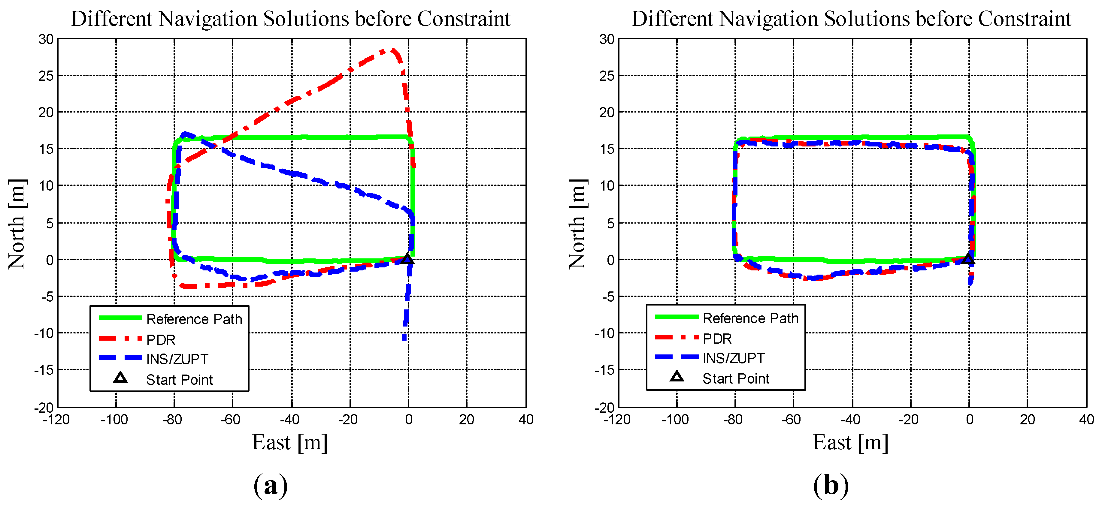
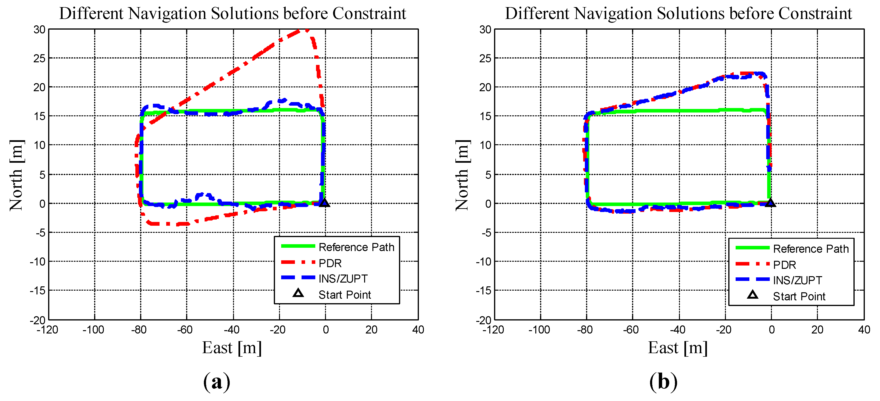
7. Results and Discussion Experimental Evaluation

For evaluating the proposed PNS approach, we conducted both the Monte Carlo simulation as well as the real field experiments. For the real experiments, first a basic experiment conducted in a GNSS available environments illustrating how the proposed algorithm works was conducted, the basic experiment was done in a GNSS available area. Then the multiple paths-based experiments were done in a GNSS-denied indoor environment.

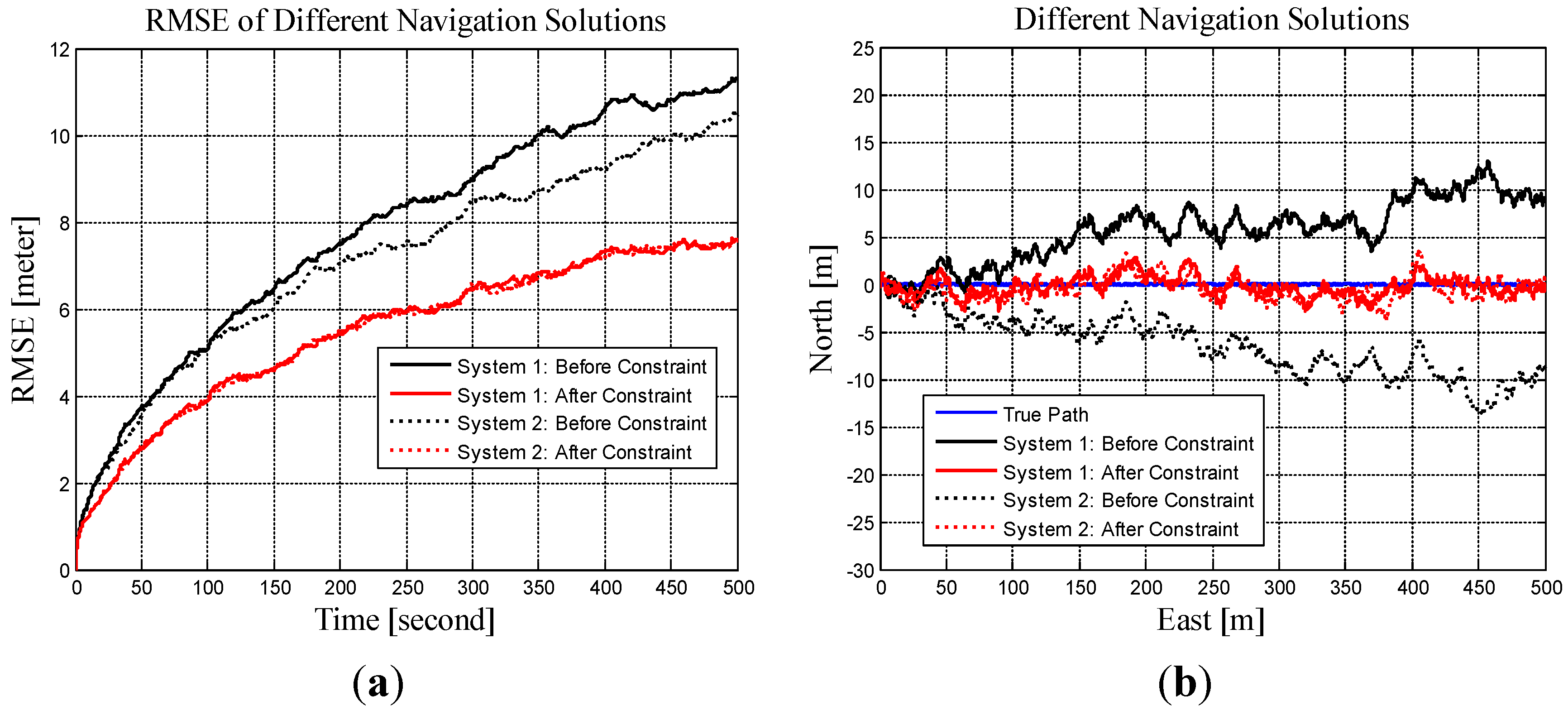
7.1. Monte Carlo Simulation

We consider the positioning of two PNSs mounted on two different parts of the user’s body. The combined positioning solutions of both systems can be expressed as:
x = [ r 1 E ( k ) r 1 N ( k ) r 2 E ( k ) r 2 N ( k ) ]
where rji (k) means the coordinate of the j-th system along the direction of i (local East or North) at time step k. We assume rji ( k ) is updated recursively as:
{ r 1 E ( k ) = r 1 E ( k 1 ) + v 1 E ( k 1 ) Δ t + s 1 E ( k 1 ) r 1 N ( k ) = r 1 N ( k 1 ) + v 1 N ( k 1 ) Δ t + s 1 N ( k 1 ) r 2 E ( k ) = r 2 E ( k 1 ) + v 2 E ( k 1 ) Δ t + s 2 E ( k 1 ) r 2 N ( k ) = r 2 N ( k 1 ) + v 2 N ( k 1 ) Δ t + s 2 N ( k 1 )
in which v j i ( k 1 ) is the speed of the j-th navigation system along the direction of i between time step k − 1 and k. Due to the errors of the used sensors, r j i is updated in consideration of noise. s j i ( k 1 ) is the position increment error of the j-th system along the direction of i. We assume the disturbed position increment, s j i , is with Gaussian distribution and can thus be expressed as:
s j i N { 0 ,    q j i }
in which q j i is the error variance of the disturbed position increment. At this time, the position error covariance, Pk , of the combined state x is updated as:
Pk = P k 1 + Q k
where P 0 is the initial position error covariance, and Q has the form:
Q = [ q 1 E 0 0 0 0 q 1 N 0 0 0 0 q 2 E 0 0 0 0 q 2 N ]
At this time, the maximum relative distance of the two systems should be a priori known, which means:
| | r 1 E ( k ) r 2 E ( k ) | | 2 + | | r 1 N ( k ) r 2 N ( k ) | | 2 d
where d is the maximum distance between the two systems. We assume that the user walks straight toward local East from the start coordinate of ( 0 , 0 ) ; the update rates of both PNSs are 100 Hz; the walking speed is set as 1 m/s, namely v 1 E = v 2 E = 1 m/s, v 1 N = v 2 N = 0 m/s; q j i = 0.05 2 m2; P 0 is initialized as a 4 × 4 null matrix; d is set as 1.5 m. We perform 30 Monte Carlo simulations, each time for 500 s.
Figure 1a shows both systems’ RMSE (Root-Mean-Square Error) values over time before and after applying the constraint approaches. The RMSE values are averaged over 30 Monte Carlo simulations. Figure 1b shows the results of one representative simulation. From Figure 1 and Figure 2 we can see that after applying the two constraint approaches, the state estimation errors could be effectively constrained.
Figure 1. (a) RMSE (Root-Mean-Square Error) versus time; (b) Trajectories of one simulation.
Micromachines 06 00926 g001
Figure 2. (a) Reference trajectory and (b) GPS (Global Position System) estimated trajectory (from Pedestrian Dead Reckoning/Global Navigation Satellite System (PDR/GNSS) system).
Micromachines 06 00926 g002

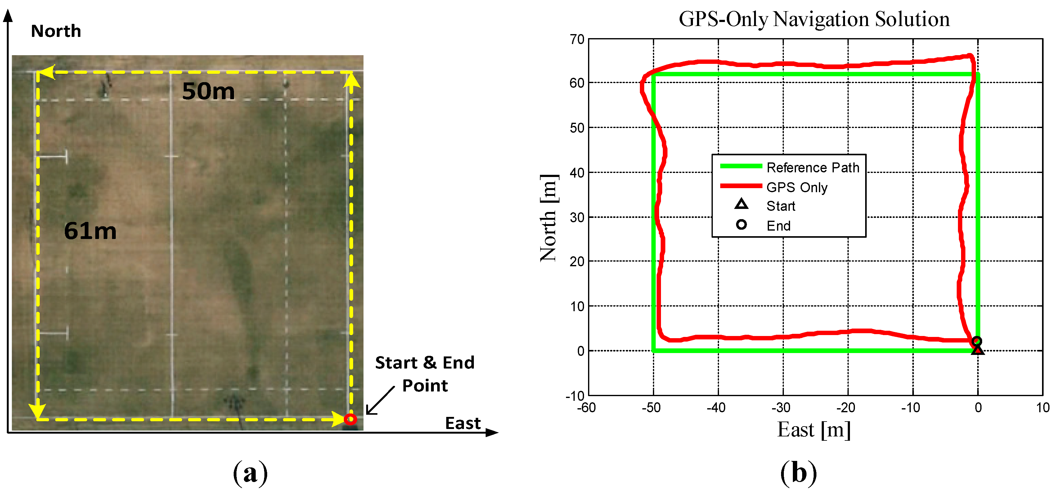
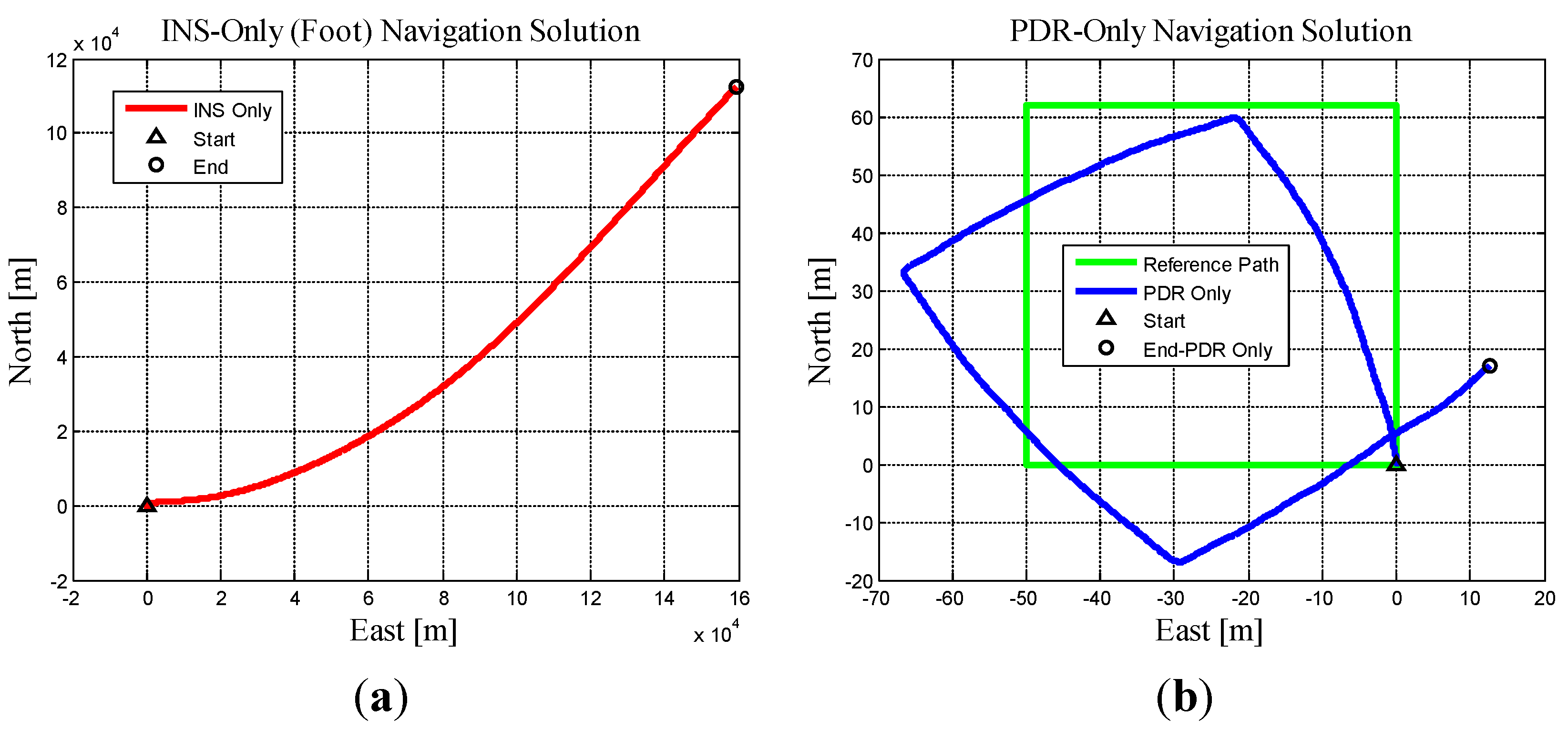
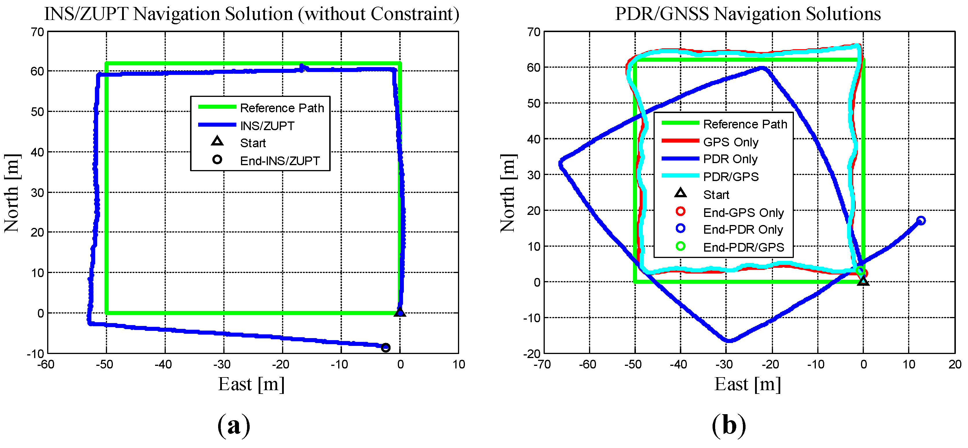
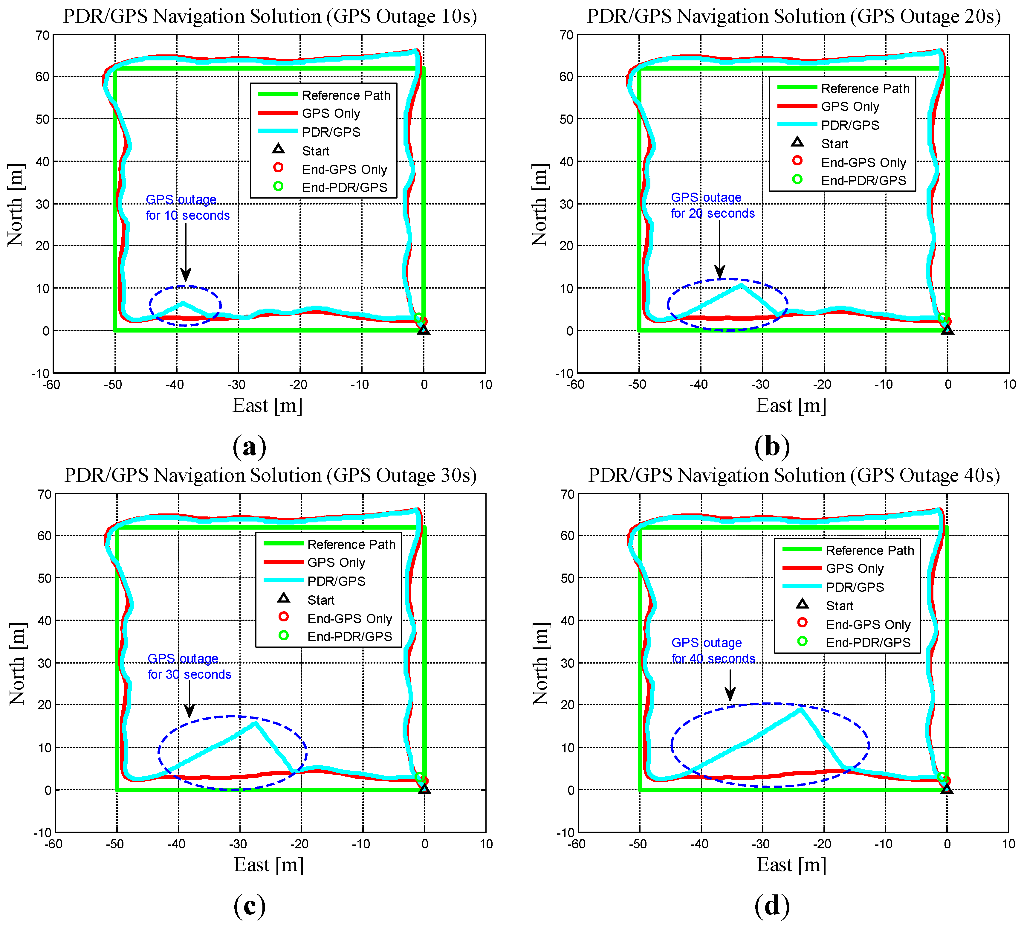
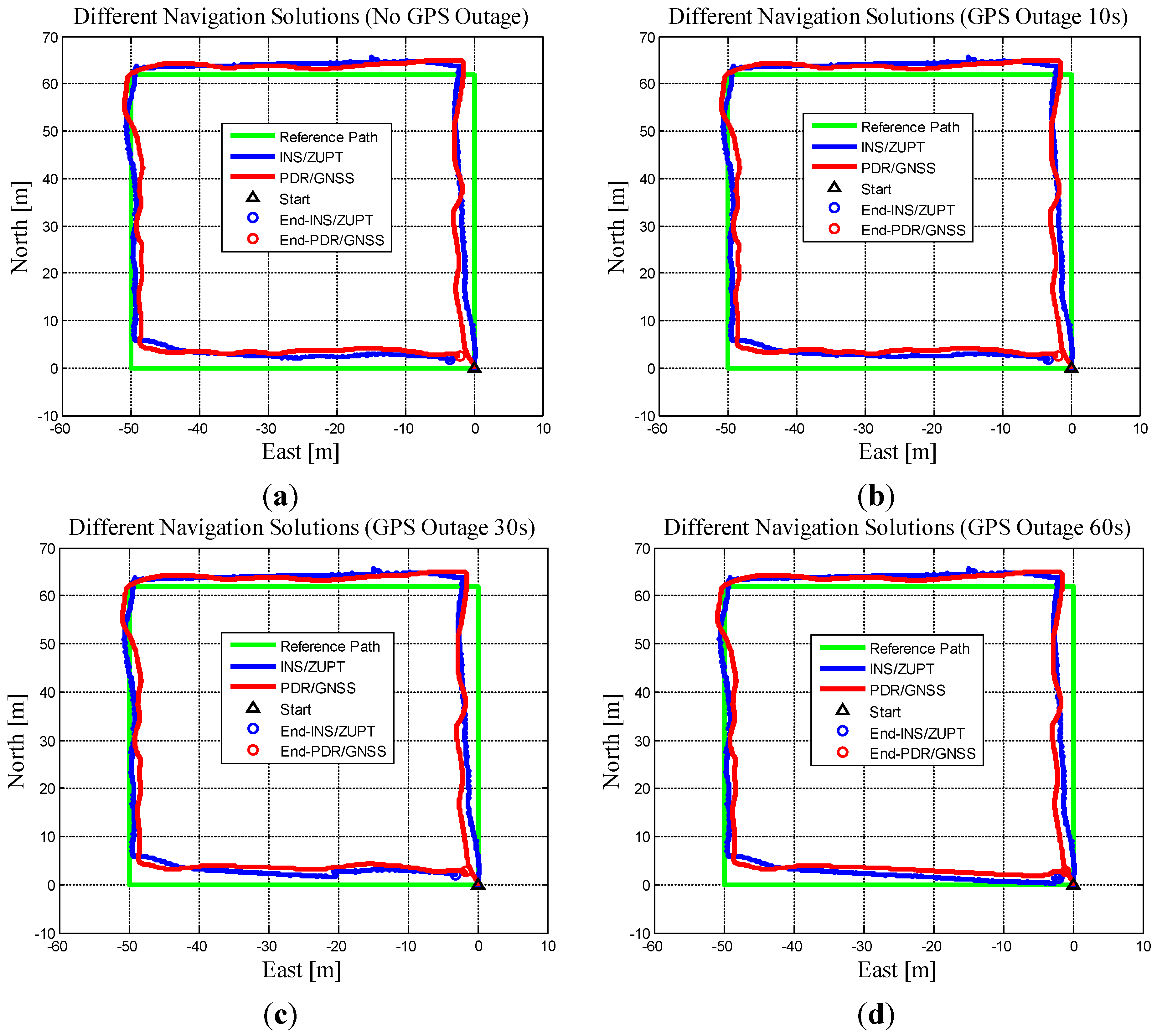
7.2. Experiments in Outdoor Environments

Two identical MEMS IMUs (embedded in two Samsung Note 2 smart-phones) including GPS (Global Position System) receivers were used to conduct the experiment. One phone was mounted on the right shoe, the other was held in the user’s right hand (keep levelled during the walking). The sampling rate of the IMU is 100 Hz, and the GPS update rate is 1 Hz. The experiment was conducted for 8 min on a standard football field (half size) within the University of Calgary’s campus area. The experiment was carried out along a rectangle-shaped line. The side of the rectangle was 61 m in length and 50 m in width, resulting in a total walking distance of 222 m. The sides of the rectangle were either parallel or vertical to the local true North and East. The ground truth, walking direction, and start and end points (which were the same) can be seen in Figure 2a.
In this research, as we have to integrate different sources of measurements together at the same time, precise synchronization or time correction between different sensors/devices is needed. For a single smartphone, because sensor sampling rate in an Android-based device is predefined and is not very stable. Programmatically, we cannot change that, at least not from application level. For solving this problem, we use the interpolation method to compensate for the uneven sensor sampling rate reflected in our smart-phones. Through interpolation, basically, we can get the sensor data with any pre-defined sampling rate.
For the synchronization issue of the sensors between two Android-based devices, there always exist an almost constant time difference between any two deceives, we need to do the temporal calibration before-hand. The temporal calibration procedure can be done easily in an open sky environment. We then use the precise GPS time recorded by two smartphones as a time reference, based on it, we can calibrate the almost unchangeable temporal bias of the sensors between the two smartphones. Due to some uncertain factors of the hardware layers of the smartphones, every time when we start recording the raw sensor data, a quite small/limited change may be added on the calibrated temporal bias. We have done tens of tests and experimentally found that such limited changes are always less than 0.1 s. If the user walks with a normal walking speed of 1 m/s, the resulting constant error distances between the two phones will always be controlled within 0.1 m. Such an error level is totally acceptable, and can be regarded as a variance of the distance constraint between the two phones.
As the GPS receiver embedded in the smart-phone is the low-cost and miniature device, this leads to limited positional accuracy. From Figure 2b we can see that the GPS could continuously provide the trajectory within ±5 m level positional accuracy during the experiments. Worth noting is that all the flowing experiment results are shown in the local geographic frame.
The following Figure 3a shows the INS-only navigation solution of foot mounted INS/ZUPT system. It can be seen that without any aiding information, the position errors diverge to hundreds of kilometers after 8 min of the experiment, due to the relative large noise ratio of the smart-phone’s low-cost MEMS inertial sensors. Figure 3b shows the PDR-only result when using the gyroscope-derived heading. As explained above that azimuth estimation is the most challenging aspect of PDR. Due to the in-run gyroscope bias, the ultimate accuracy and quality of the navigation solution degraded gradually with the walked distance. The position error at the end of the test is around 20 m.
Figure 4a shows the INS/ZUPT system’s navigation result. When the INS was frequently aided by ZUPTs, the error accumulation is well bounded for a short period of time (within 5 min). However, when the user walked for a long time, small error accumulation was noticed, these errors were primarily driven by the errors in the heading estimation as well as the large in-run bias instability of the inertial sensor, leading to position error on the order of 5 m after about 5 min of walking. The maximum error was seen at the end of the walk with almost 10 m. Such error level is reasonable given the quality of the used smart-phone’s cheap MEMS inertial sensors. As we don’t have reference trajectory with which to evaluate the entire trip’s absolute accuracy, however, the user ended the walking very close to the original starting point (0, 0, 0), the INS/ZUPT derived position was displaced about 10 m, indicating a probable accuracy of approximately 4 percent of the traveled distance.
Figure 4b shows the navigation results obtained from the PDR/GNSS sub-system when there is no GPS signal outages. As can be seen from the figure that the integrated system performed quite well which was actually expected when aided by periodical GPS derived positions. Since the satellite visibility is relatively good over the trajectory, to assess the performance of the constraint algorithm’s positioning capability during GPS signal outage periods, the GPS outages are manually simulated for 10, 20, 30 and 40 s, respectively.
Figure 3. (a) INS Only navigation solution (from Inertial Navigation System/Zero Velocity Update (INS/ZUPT) system); (b) PDR only navigation solution (from PDR/GNSS system).
Micromachines 06 00926 g003
Figure 4. (a) INS/ZUPT system’s navigation solution; (b) PDR/GNSS system’s integrated navigation solution.
Micromachines 06 00926 g004
Figure 5 shows the PDR/GNSS sub-system’s navigation solutions for the four GPS outage scenarios, we can see that when there is no GPS update, the position result will diverge up to 20 m during the GPS outage period for 40 s. With the same divergence trend, worse results will obtained when simulating GPS outage for longer duration. Figure 6 below shows the KF derived positions after applying the state constraint algorithm. Figure 6a presents the constrained position estimates when there is no GPS signal outage, Figure 6b–d, respectively, give the constrained position estimates when GPS outages are simulated by 10, 30 and 60 s. The constraint’s update rate is the same as the user’s step-rate, namely the constraint is applied when a step is detected as well as the horizontal distance between the two systems is larger than the predefined d (1.5 m).
As can be noted from Figure 6, the positioning results from both PDR/GNSS and INS/ZUPT systems are similar, both performed quite well and remained closely aligned with the reference solution with acceptable deviations visible at different portions of the trajectories. The maximum position errors of PDR/GNSS and INS/ZUPT systems are on the order of 5 m. The state constraint algorithm allows the correct adjustments in situations when detecting the spatial distances between the two sub-systems are larger than 1.5 m, then diminishing the position errors in each system, all of the track closure errors of both systems significantly bounded. As visible from Figure 5, when there is GPS outage, through applying the state constraint algorithm, the PDR/GNSS sub-system’s horizontal position errors can be greatly corrected during the GPS outage period comparing with the results shown in Figure 5 (without applying the constraint algorithm). Similarly, the position errors remained under 5 m, which is significant given that the GPS outage lasted for about 60 s.
From the above experimental results, we can conclude that when GPS is available, the GPS position will be periodically used to update the hand-held smart-phone’s PDR/GNSS estimate, therefore, the PDR/GNSS system’s state error covariance P pdr could always be restricted in a relatively small value. However, for the foot-mounted INS/ZUPT system, due to the reason that the heading of the system is not observable during ZUPT as well as the large in-run bias instability of the inertial sensor, both could result into the INS/ZUPT system’s position error covariance P ins diverges slowly and gradually. According to Equation (3.8), P 1 can be regarded as the weighting factor, which is the inverse of the combined navigation state covariance matrix P . At this time, the inverse of P pdr is much bigger than the inverse of P ins , therefore the position of PDR/GNSS system is much accurate than that of the INS/ZUPT system, then the final positions of the two systems when using the state constraint algorithm will more “trust” the PDR/GNSS system’s result.
Figure 5. PDR/GNSS system’s navigation solutions for simulated different GPS Outages of (a) 10 s; (b) 20 s; (c) 30 s; (d) 40 s.
Micromachines 06 00926 g005
Figure 6. Two systems’ navigation solutions with state constraint for simulated GPS outage of (a) 10 s; (b) 20 s; (c) 30 s; (d) 40 s.
Micromachines 06 00926 g006
On the contrary, when GPS is not available, the INS/ GNSS system’s position error covariance (standard deviation) P pdr will increase quickly, and benefiting from the preceding position correction by the state constraint algorithm as well as the periodical usage of ZUPT, the INS/ZUPT system’s position error covariance P ins will not increase quickly and at this time, during the GPS outage, the inverse of P ins is much bigger, therefore the position estimate of INS/ZUPT system is much accurate than that of the PDR/GNSS system, then the final positions of the two systems when using the state constraint algorithm will more “trust” the INS/ZUPT system’s result.

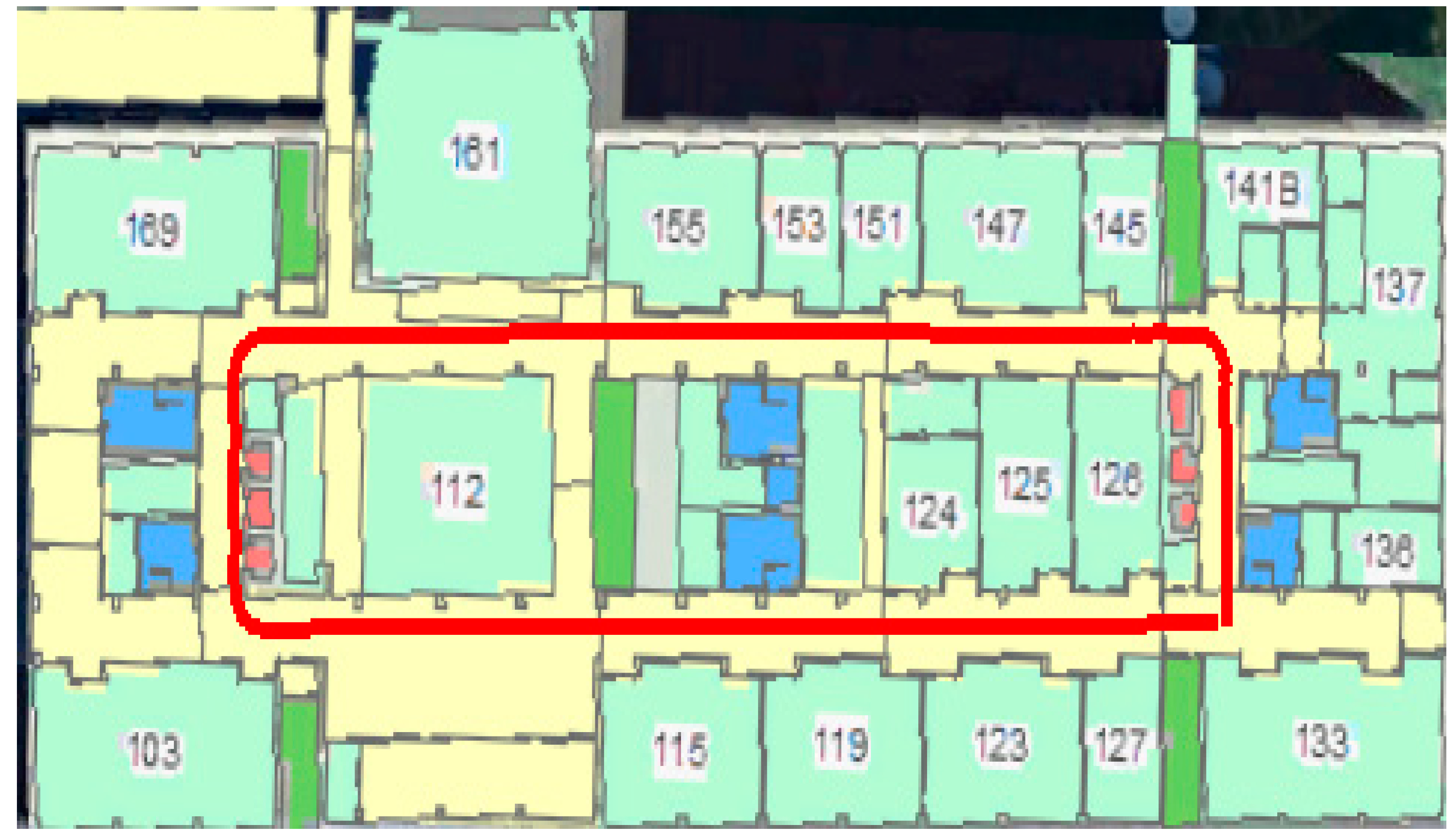
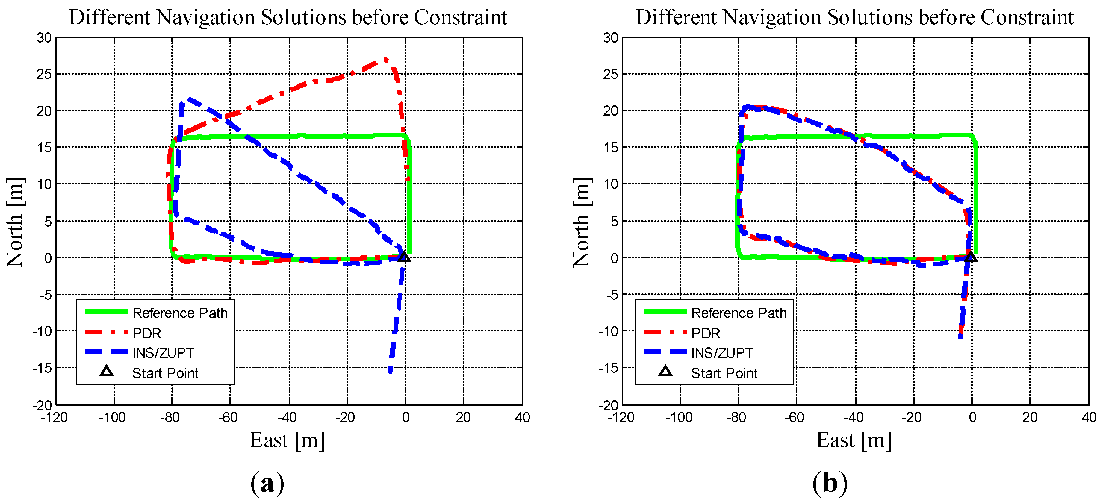
7.3. Experiments in Indoor Environments

The preceding open sky-based field experiment as well as its results have well illustrated the basic working principle and the efficacy of the proposed constraint approach. Although the results seem promising with/without the simulated GPS outages, however, in general, the one experimental trajectory is not enough to support the significant conclusions. Also, some researchers may challenge that why not fuse the GNSS and INS/ZUPT directly. In order to adequately back up the conclusions drawn from the above experiment, as well as demonstrate that the navigation solution derived through the integration of multiple PNSs is much more accurate and robust than that of using only a standalone PNS when there is no external aiding information, such as GNSS, WiFi, etc.
In this subsection, we performed several indoor experiments when GNSS was totally unavailable. Two late model smart-phones (Xiaomi Mi 4 (Xiaomi, Beijing, China)) using STMicroelectronics MEMS IMUs (STMicroelectronics, Geneva, Switzerland) were used to conduct the multiple paths-based experiments in an indoor area. The gyroscope embedded in the Mi 4 has much lower noise density as well as bias stability compared with the gyroscope embedded in the Samsung Note 2 (Samsung, Suwon, South Korea) for the experiment given in Subsection 7.2. The experiments were conducted in the Energy Environment Experiential Learning (EEEL) at the University of Calgary. The ground truth for the experiment is about 80 m × 16.5 m. Six identical trajectories were used to test the performance of proposed constraint approach. The reference trajectory and the first floor plan of the EEEL building can be seen in the following Figure 7.
Figure 7. Reference trajectory at the energy environment experiential learning (EEEL).
Micromachines 06 00926 g007
Also, in order to quantitatively show the performance of the proposed algorithm, we need to obtain reference trajectories/coordinates for further error analysis. In this research, we adopt the indoor map-aided PDR method for generating relatively precise reference trajectories. We make full use of the fact that most of the indoor corridors are straight as well as the positions of corners and intersections are known on specific indoor maps. At any moment, when detecting the user is walking along a straight line/corridor, the user’s walking heading for the PDR update will be “locked” in a specific value according to the indoor map. In this experiment, any momentary headings derived from the gyroscope are all corresponding to one of the four dominate directions (in degree), 0/360, 90, 180 and 270. Meanwhile, at any time when detecting the heading change of the user, the specific corners and intersections will also be detected, which can be regarded as “landmarks” to further correct the PDR-derived positions.
The following Figure 8, Figure 9, Figure 10, Figure 11, Figure 12 and Figure 13 respectively show the six trajectories-derived navigation solutions. Each figure gives both the positioning results of both PDR and INS/ZUPT navigation systems before and after applying the proposed state constraint algorithm. Correspondingly, the positioning performances using different approaches in the six trajectories can be seen in Table 1.
Figure 8. Trajectory I: Two systems’ navigation solutions. (a) Before constraint; (b) After constraint.
Micromachines 06 00926 g008
Figure 9. Trajectory II: Two systems’ navigation solutions. (a) Before constraint; (b) After constraint.
Micromachines 06 00926 g009
Figure 10. Trajectory III: Two systems’ navigation solutions. (a) Before constraint; (b) After constraint.
Micromachines 06 00926 g010
Figure 11. Trajectory IV: Two systems’ navigation solutions. (a) Before constraint; (b) After constraint.
Micromachines 06 00926 g011
Figure 12. Trajectory V: Two systems’ navigation solutions. (a) Before constraint; (b) After constraint.
Micromachines 06 00926 g012
Figure 13. Trajectory VI: Two systems’ navigation solutions. (a) Before constraint; (b) After constraint.
Micromachines 06 00926 g013
Table 1. Positioning performance using different algorithms in the six different trajectories.
TrajectorySystemAlgorithmError (m)
MaximumMinimumMeanRMS
Trajectory IHand-heldBefore Constraint13.8630.3196.8527.515
After Constraint9.6390.2584.6005.036
Foot-MountedBefore Constraint15.0280.3196.0297.098
After Constraint9.8820.3194.6525.077
Trajectory IIHand-heldBefore Constraint8.1490.5413.6074.149
After Constraint6.7780.8722.7042.978
Foot-MountedBefore Constraint14.8380.0395.3946.641
After Constraint7.1980.0392.6902.988
Trajectory IIIHand-heldBefore Constraint12.1611.2614.7495.841
After Constraint3.6890.1782.0422.276
Foot-MountedBefore Constraint7.4570.9814.3944.569
After Constraint3.7200.1942.0982.326
Trajectory IVHand-heldBefore Constraint13.6710.1155.1726.498
After Constraint2.6710.0211.1771.347
Foot-MountedBefore Constraint10.9320.0273.6834.813
After Constraint2.8570.0741.1711.313
Trajectory VHand-heldBefore Constraint15.8250.0435.7307.414
After Constraint6.6060.0432.5833.210
Foot-MountedBefore Constraint1.7910.0140.7160.832
After Constraint6.9230.3162.4583.235
Trajectory VIHand-heldBefore Constraint20.3190.0118.40910.123
After Constraint5.3900.0112.4252.689
Foot-MountedBefore Constraint12.8690.2953.6865.555
After Constraint5.1920.3192.3342.611
The navigation performances using the two different approaches (with/without constraint) in the six trajectories are depicted in the above Table 1. As can be seen from Figure 8, Figure 9, Figure 10, Figure 11, Figure 12 and Figure 13 and Table 1, the constraint approach has improved the navigation performances of both PDR and INS/ZUPT systems in the trajectories of I, II, III, IV and VI, especially has significantly improved those in the trajectories of III, IV and VI. Only the INS/ZUPT navigation system’ performance in trajectory V has degraded, with RMS (Root-Mean-Square) values degraded from 0.732 to 3.235 m, mean values degraded from 0.616 to 2.458 m, however, such error level is still acceptable given the application of pedestrian indoor navigation. On the contrary, in the same trajectory V, the PDR performance has been greatly improved, with RMS values improved from 7.414 to 3.210 m, mean values improved from 5.730 to 2.583 m. From the robustness point of view, the integrated navigation systems are more robust than each individual system through applying the proposed constraint KF approach.
From Figure 8, Figure 9, Figure 10, Figure 11, Figure 12 and Figure 13 and Table 1, it can be summarized that on average the navigation results using the constraint approach offer obvious improvement over the navigation results without using the proposed constraint approach, six out of six being improved with the PDR system, and five out of six being improved with the INS/ZUPT system. Due to our limited sample size of six experiments, the above given numbers should not be regarded as having any significance in the aspect of statistics, however, the six experiments do show the improvement that is possible with the proposed constraint approach for the integration of multiple pedestrian navigation systems.

8. Conclusions

This paper presents a novel pedestrian navigation prototype through integrating the navigation solutions from two individual PNSs, namely the upper body mounted PDR/GNSS system and the foot-mounted INS/ZUPT system. A nonlinear inequality distance constraint between the two systems’ positioning estimates are explored. The state constraint Kalman filter is used to fuse the two systems’ navigation information and to diminish the positioning errors of both systems. The proposed new pedestrian navigation prototype was tested through both the Monte Carlo simulations and several real field experiments. Through using the constraint algorithm, both navigation systems’ positioning accuracy could be well improved. Future work includes the integration of three or more systems to compose a more robust PNS prototype. Also, long term indoor/outdoor experiments will be done to evaluate the performance of the integrated PNS prototype.

Acknowledgments

This research is sponsored by both Naser El-Sheimy and the China Scholarship Council (CSC). Trusted Positioning Inc. (Acquired by InvenSense (San Jose, CA, USA)) is appreciated for providing the “TPI Android Logger” software to record the raw data of the used sensors.

Author Contributions

The first author Haiyu Lan conceived the idea of this paper. Numerical simulations, real field experiments, and data processing were performed by Haiyu Lan, Chunyang Yu, You Li, and Yuan Zhuang. Naser El-Sheimy supervised the whole work and provided very important technical feedbacks. All the five authors have contributed to the writing of the paper.

Conflicts of Interest

The authors declare no conflict of interest.

References

  1. Rantakokko, J.; Strömbäck, P.; Emilsson, E.; Rydell, J. Soldier Positioning in Gnss-Denied Operations. In Proceedings of the Sensors and Electronics Technology Panel Symposium (SET-168) on Navigation Sensors and Systems in GNSS Denied Environments, Izmir, Turkey, 8–9 October 2012.
  2. Hepsaydir, E. Mobile Positioning in CDMA Cellular Networks. In Proceedings of the 50th Vehicular Technology Conference, Amsterdam, The Netherlands, 19–22 September 1999; pp. 795–799.
  3. Yamamoto, R.; Matsutani, H.; Matsuki, H.; Oono, T.; Ohtsuka, H. Position Location Technologies Using Signal Strength in Cellular Systems. In Proceedings of the 53rd Vehicular Technology Conference, Mexico City, Mexico, 6–9 May 2001; pp. 2570–2574.
  4. Hari, K.; Nilsson, J.-O.; Skog, I.; Händel, P.; Rantakokko, J.; Prateek, G. A prototype of a first-responder indoor localization system. J. Indian Inst. Sci. 2013, 93, 511–520. [Google Scholar]
  5. Ruiz, A.R.J.; Granja, F.S.; Honorato, J.C.P.; Rosas, J.I.G. Accurate pedestrian indoor navigation by tightly coupling foot-mounted IMU and RFID measurements. IEEE Trans. Instrum. Meas. 2012, 61, 178–189. [Google Scholar] [CrossRef]
  6. Li, Y.; Zhuang, Y.; Lan, H.; Zhang, P.; Niu, X.; El-Sheimy, N. Wifi-aided magnetic matching for indoor navigation with consumer portable devices. Micromachines 2015, 6, 747–764. [Google Scholar] [CrossRef]
  7. Shin, E.-H. Estimation Techniques for Low-Cost Inertial Navigation; UCGE Report No. 20219; University of Calgary: Calgary, Canada, 2005. [Google Scholar]
  8. Foxlin, E. Pedestrian tracking with shoe-mounted inertial sensors. IEEE Computer Graph. Appl. 2005, 25, 38–46. [Google Scholar] [CrossRef]
  9. Nilsson, J.-O.; Skog, I.; Händel, P. A Note on the Limitations of Zupts and the Implications on Sensor Error Modeling. In Proceeding of the 2012 International Conference on Indoor Positioning and Indoor Navigation, Sydney, Australia, 13–15 November 2012.
  10. Jirawimut, R.; Ptasinski, P.; Garaj, V.; Cecelja, F.; Balachandran, W. A method for dead reckoning parameter correction in pedestrian navigation system. IEEE Trans. Instrum. Meas. 2003, 52, 209–215. [Google Scholar] [CrossRef]
  11. Mezentsev, O.; Collin, J.; Lachapelle, G. Pedestrian dead reckoning—A solution to navigation in GPS signal degraded areas? Geomatica 2005, 59, 175–182. [Google Scholar]
  12. Lan, H.; Yu, C.; El-Sheimy, N. An Integrated PDR/GNSS Pedestrian Navigation System. In China Satellite Navigation Conference (CSNC) 2015 Proceedings: Volume III; Springer-Verlag: Berlin, Germany, 2015; pp. 677–690. [Google Scholar]
  13. Gabaglio, V.; Ladetto, Q.; van Seeters, J. Pedestrian Navigation Method and Apparatus Operative in a Dead Reckoning Mode. U.S. Patent No. 6,826,477, 23 April 2001. [Google Scholar]
  14. Beauregard, S.; Haas, H. Pedestrian dead reckoning: A basis for personal positioning. In Proceedings of the 3rd Workshop on Positioning, Navigation and Communication, Hannover, Germany, 16 March 2006; pp. 27–35.
  15. Renaudin, V.; Susi, M.; Lachapelle, G. Step length estimation using handheld inertial sensors. Sensors 2012, 12, 8507–8525. [Google Scholar] [CrossRef] [PubMed]
  16. Chang, H.-W.; Georgy, J.; El-Sheimy, N. Techniques for 3D Misalignments Calculation for Portable Devices in Cycling Applications. In Proceedings of the 26th International Technical Meeting of The Satellite Division of the Institute of Navigation (ION GNSS+ 2013), Nashville, TN, USA, 16–20 September 2013; pp. 2862–2867.
  17. Omr, M.; Georgy, J.; Noureldin, A. Using Multiple Sensor Triads for Enhanced Misalignment Estimation for Portable and Wearable Devices. In Proceedings of the Position, Location and Navigation Symposium, Monterey, CA, USA, 5–8 May 2014; pp. 1146–1154.
  18. Zhuang, Y.; Lan, H.; Li, Y.; El-Sheimy, N. PDR/INS/WiFi integration based on handheld devices for indoor pedestrian navigation. Micromachines 2015, 6, 793–812. [Google Scholar] [CrossRef]
  19. Lan, H.; El-Sheimy, N. A State Constraint Kalman Filter for Pedestrian Navigation with Low Cost Mems Inertial Sensors. In Proceedings of the 27th International Technical Meeting of The Satellite Division of the Institute of Navigation, Tampa, FL, USA, 8–12 September 2014; pp. 579–589.
  20. Brand, T.J.; Phillips, R.E. Foot-to-Foot Range Measurement as an Aid to Personal Navigation. In Proceedings of the 59th Annual Meeting of The Institute of Navigation and CIGTF 22nd Guidance Test Symposium, Albuquerque, NM, USA, 23–25 June 2003; pp. 113–121.
  21. Bancroft, J.B. Multiple Inertial Measurement Unit Integration for Pedestrian Navigation; UCGE Report No. 20320; University of Calgary: Calgary, Canada, 2010. [Google Scholar]
  22. Skog, I.; Nilsson, J.-O.; Zachariah, D.; Handel, P. Fusing the Information from Two Navigation Systems Using an Upper Bound on Their Maximum Spatial Separation. In Proceedings of the Indoor Positioning and Indoor Navigation, Sydney, Australia, 13–15 November 2012; pp. 1–5.
  23. Laverne, M.; George, M.; Lord, D.; Kelly, A.; Mukherjee, T. Experimental Validation of Foot to Foot Range Measurements in Pedestrian Tracking. In Proceedings of the 24th International Technical Meeting of The Satellite Division of the Institute of Navigation, Portland, OR, USA, 20–23 September 2011.
  24. Zampella, F.; De Angelis, A.; Skog, I.; Zachariah, D.; Jiménez, A. A Constraint Approach for UWB and PDR Fusion. In Proceedings of the International Conference on Indoor Positioning and Indoor Navigation, Sydney, NSW, Australia, 13–15 November 2012.
  25. Simon, D.; Chia, T.L. Kalman filtering with state equality constraints. IEEE Trans. Aerosp. Electron. Syst. 2002, 38, 128–136. [Google Scholar] [CrossRef]
  26. Anderson, B.D.; Moore, J.B. Optimal Filtering; Courier Dover Publications: Mineola, NY, USA, 2012. [Google Scholar]
  27. Fletcher, R. Practical Methods of Optimization; John Wiley & Sons: Hoboken, NJ, USA, 2013. [Google Scholar]
  28. Sun, F.; Lan, H.; Yu, C.; El-Sheimy, N.; Zhou, G.; Cao, T.; Liu, H. A robust self-alignment method for ship’s strapdown ins under mooring conditions. Sensors 2013, 13, 8103–8139. [Google Scholar] [CrossRef] [PubMed]
  29. El-Sheimy, N. Inertial Techniques and INS/DGPS Integration. In Engo 623-Course Notes; University of Calgary: Calgary, Canada, 2003; pp. 170–182. [Google Scholar]
  30. Noureldin, A.; Karamat, T.B.; Georgy, J. Fundamentals of Inertial Navigation, Satellite-based Positioning and Their Integration; Springer-Verlag: Berlin, Germany, 2013. [Google Scholar]
  31. Fischer, C.; Talkad Sukumar, P.; Hazas, M. Tutorial: Implementation of a pedestrian tracker using foot-mounted inertial sensors. IEEE Pervasive Comput. 2012, 12, 17–27. [Google Scholar] [CrossRef]
  32. Jimenez, A.R.; Seco, F.; Prieto, J.C.; Guevara, J. Indoor Pedestrian Navigation Using an INS/EKF framework for Yaw Drift Reduction and a Foot-Mounted IMU. In Proceedings of the 2010 7th Workshop on Positioning Navigation and Communication, Dresden, Germany, 11–12 March 2010; pp. 135–143.
  33. Godha, S.; Lachapelle, G. Foot mounted inertial system for pedestrian navigation. Meas. Sci. Technol. 2008, 19, 075202. [Google Scholar] [CrossRef]
  34. Skog, I.; Handel, P.; Nilsson, J.-O.; Rantakokko, J. Zero-velocity detection—An algorithm evaluation. IEEE Trans. Biomed. Eng. 2010, 57, 2657–2666. [Google Scholar] [CrossRef] [PubMed]
  35. Bao, H.; Wong, W.-C. A novel map-based dead-reckoning algorithm for indoor localization. J. Sens. Actuator Netw. 2014, 3, 44–63. [Google Scholar] [CrossRef]
  36. Gabaglio, V.; Ladetto, Q.; Merminod, B. Kalman filter approach for augmented GPS pedestrian navigation. Available online: http://quentin.ladetto.ch/publications/kalapproach.pdf (accessed on 12 July 2015).

