
A Computational Evaluation of Minimum Feature Size in Projection Two-Photon Lithography for Rapid Sub-100 nm Additive Manufacturing

Abstract
:1. Introduction
2. Materials and Methods
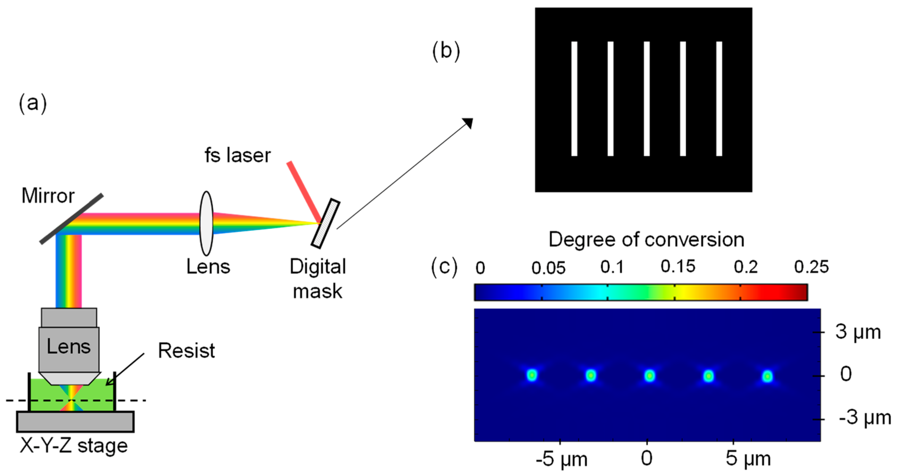
2.1. P-TPL Process
2.2. Finite Elements Model of P-TPL
2.3. Full-Factorial Design of Computational Experiments
2.4. Dynamic Prgramming Approach
3. Results and Discussion
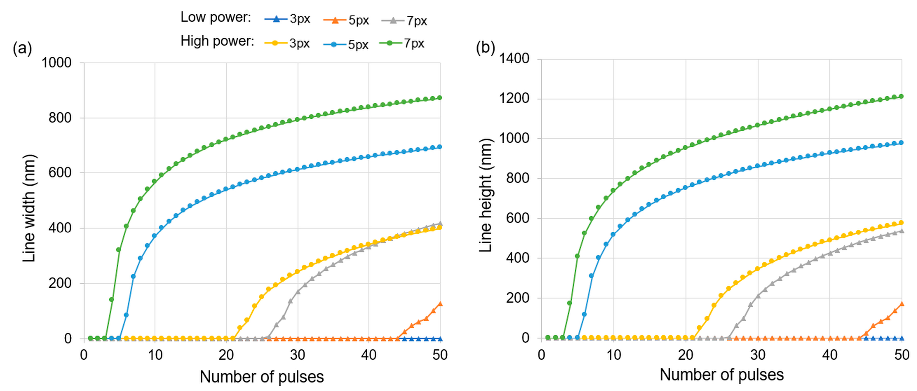
3.1. Effect of Number of Pulses
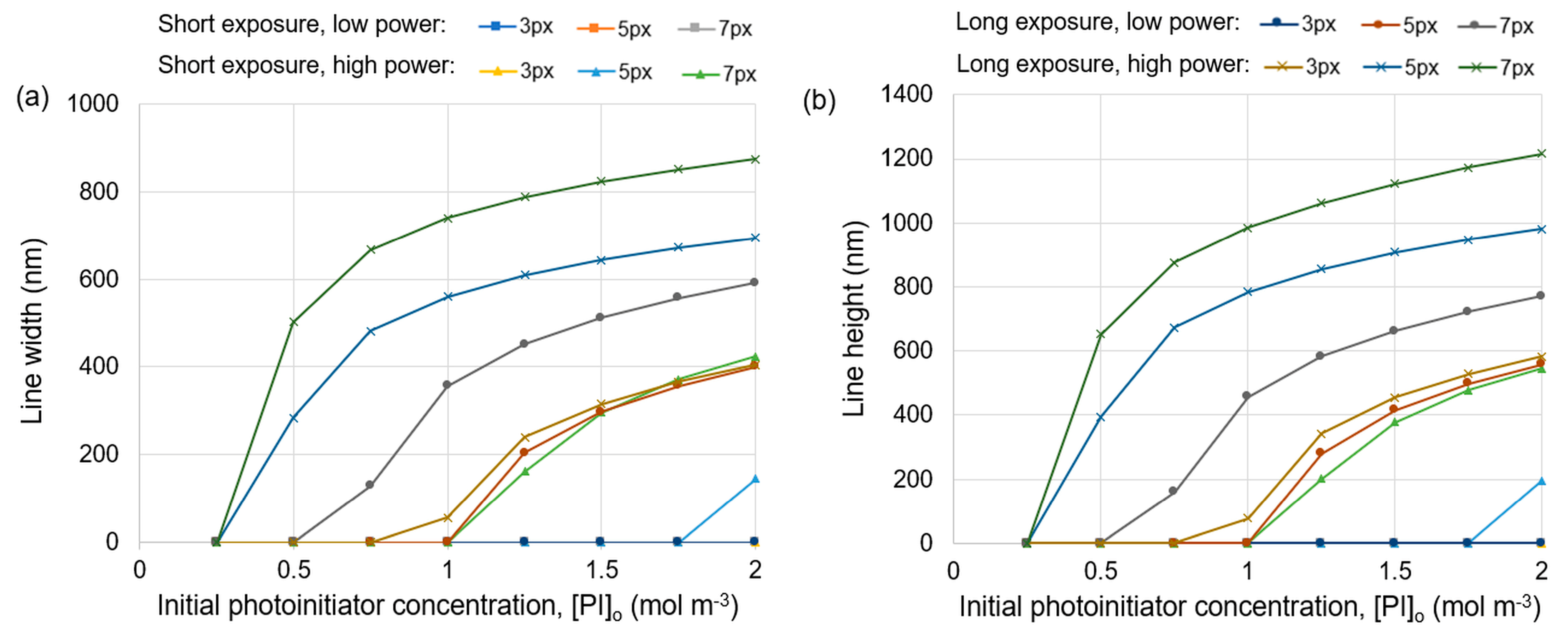
3.2. Effect of Photoinitiator Concentration
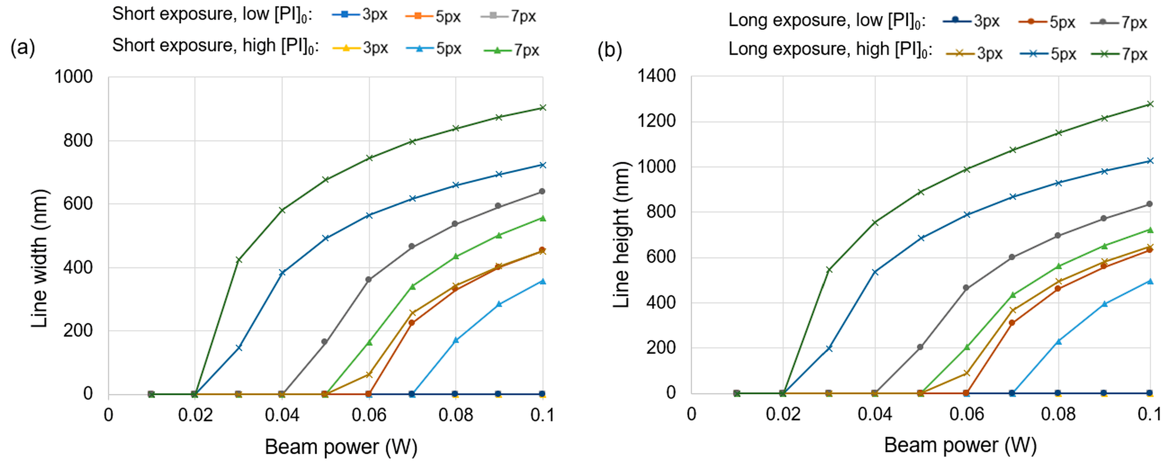
3.3. Effect of Optical Power
3.4. Sub-100 nm Regime
3.5. Insights for Rapid Sub-100 nm 3D Printing
3.6. Demonstration of Explanatory Power of the Simulations
4. Conclusions
Author Contributions
Funding
Data Availability Statement
Acknowledgments
Conflicts of Interest
References
- Harinarayana, V.; Shin, Y.C. Two-photon lithography for three-dimensional fabrication in micro/nanoscale regime: A comprehensive review. Opt. Laser Technol. 2021, 142, 107180. [Google Scholar] [CrossRef]
- Malinauskas, M.; Farsari, M.; Piskarskas, A.; Juodkazis, S. Ultrafast laser nanostructuring of photopolymers: A decade of advances. Phys. Rep. 2013, 533, 1–31. [Google Scholar] [CrossRef]
- Zheng, L.; Kurselis, K.; El-Tamer, A.; Hinze, U.; Reinhardt, C.; Overmeyer, L.; Chichkov, B. Nanofabrication of high-resolution periodic structures with a gap size below 100 nm by two-photon polymerization. Nanoscale Res. Lett. 2019, 14, 1–9. [Google Scholar] [CrossRef] [PubMed]
- Baldacchini, T. Three-Dimensional Microfabrication Using Two-Photon Polymerization: Fundamentals, Technology, and Applications; William Andrew: Waltham, MA, USA, 2015. [Google Scholar]
- Selimis, A.; Mironov, V.; Farsari, M. Direct laser writing: Principles and materials for scaffold 3D printing. Microelectron. Eng. 2015, 132, 83–89. [Google Scholar] [CrossRef]
- Li, J.; Thiele, S.; Quirk, B.C.; Kirk, R.W.; Verjans, J.W.; Akers, E.; Bursill, C.A.; Nicholls, S.J.; Herkommer, A.M.; Giessen, H. Ultrathin monolithic 3D printed optical coherence tomography endoscopy for preclinical and clinical use. Light Sci. Appl. 2020, 9, 124. [Google Scholar] [CrossRef] [PubMed]
- Lay, C.L.; Koh, C.S.L.; Lee, Y.H.; Phan-Quang, G.C.; Sim, H.Y.F.; Leong, S.X.; Han, X.; Phang, I.Y.; Ling, X.Y. Two-Photon-Assisted Polymerization and Reduction: Emerging Formulations and Applications. ACS Appl. Mater. Interfaces 2020, 12, 10061–10079. [Google Scholar] [CrossRef]
- Soreni-Harari, M.; St. Pierre, R.; McCue, C.; Moreno, K.; Bergbreiter, S. Multimaterial 3D Printing for Microrobotic Mechanisms. Soft Robot. 2020, 7, 59–67. [Google Scholar] [CrossRef]
- Oakdale, J.S.; Smith, R.F.; Forien, J.B.; Smith, W.L.; Ali, S.J.; Bayu Aji, L.B.; Willey, T.M.; Ye, J.; Van Buuren, A.W.; Worthington, M.A.; et al. Direct Laser Writing of Low-Density Interdigitated Foams for Plasma Drive Shaping. Adv. Funct. Mater. 2017, 27, 1702425. [Google Scholar] [CrossRef]
- Gonzalez-Hernandez, D.; Varapnickas, S.; Bertoncini, A.; Liberale, C.; Malinauskas, M. Micro-Optics 3D Printed via Multi-Photon Laser Lithography. Adv. Opt. Mater. 2023, 11, 2201701. [Google Scholar] [CrossRef]
- Bauer, J.; Crook, C.; Baldacchini, T. A sinterless, low-temperature route to 3D print nanoscale optical-grade glass. Science 2023, 380, 960–966. [Google Scholar] [CrossRef]
- Wang, H.; Zhang, W.; Ladika, D.; Yu, H.; Gailevičius, D.; Wang, H.; Pan, C.F.; Nair, P.N.S.; Ke, Y.; Mori, T. Two-Photon Polymerization Lithography for Optics and Photonics: Fundamentals, Materials, Technologies, and Applications. Adv. Funct. Mater. 2023, 2214211. [Google Scholar] [CrossRef]
- Schulz, J.; Vaidya, S.; Jörg, C. Topological photonics in 3D micro-printed systems. APL Photonics 2021, 6, 080901. [Google Scholar] [CrossRef]
- Xia, X.; Afshar, A.; Yang, H.; Portela, C.M.; Kochmann, D.M.; Di Leo, C.V.; Greer, J.R. Electrochemically reconfigurable architected materials. Nature 2019, 573, 205–213. [Google Scholar] [CrossRef] [PubMed]
- Meza, L.R.; Das, S.; Greer, J.R. Strong, lightweight, and recoverable three-dimensional ceramic nanolattices. Science 2014, 345, 1322–1326. [Google Scholar] [CrossRef]
- Bauer, J.; Schroer, A.; Schwaiger, R.; Kraft, O. Approaching theoretical strength in glassy carbon nanolattices. Nat. Mater. 2016, 15, 438–443. [Google Scholar] [CrossRef] [PubMed]
- Bauer, J.; Crook, C.; Izard, A.G.; Eckel, Z.C.; Ruvalcaba, N.; Schaedler, T.A.; Valdevit, L. Additive manufacturing of ductile, ultrastrong polymer-derived nanoceramics. Matter 2019, 1, 1547–1556. [Google Scholar] [CrossRef]
- Jonušauskas, L.; Juodkazis, S.; Malinauskas, M. Optical 3D printing: Bridging the gaps in the mesoscale. J. Opt. 2018, 20, 053001. [Google Scholar] [CrossRef]
- Kiefer, P.; Hahn, V.; Nardi, M.; Yang, L.; Blasco, E.; Barner-Kowollik, C.; Wegener, M. Sensitive photoresists for rapid multiphoton 3D laser micro-and nanoprinting. Adv. Opt. Mater. 2020, 8, 2000895. [Google Scholar] [CrossRef]
- Wloka, T.; Gottschaldt, M.; Schubert, U.S. From light to structure: Photo initiators for radical two-photon polymerization. Chem. –A Eur. J. 2022, 28, e202104191. [Google Scholar] [CrossRef]
- Saha, S.K.; Wang, D.; Nguyen, V.H.; Chang, Y.; Oakdale, J.S.; Chen, S.-C. Scalable submicrometer additive manufacturing. Science 2019, 366, 105–109. [Google Scholar] [CrossRef]
- Hahn, V.; Kiefer, P.; Frenzel, T.; Qu, J.; Blasco, E.; Barner-Kowollik, C.; Wegener, M. Rapid Assembly of Small Materials Building Blocks (Voxels) into Large Functional 3D Metamaterials. Adv. Funct. Mater. 2020, 1907795. [Google Scholar] [CrossRef]
- Ouyang, W.; Xu, X.; Lu, W.; Zhao, N.; Han, F.; Chen, S.-C. Ultrafast 3D nanofabrication via digital holography. Nat. Commun. 2023, 14, 1716. [Google Scholar] [CrossRef]
- Somers, P.; Liang, Z.; Johnson, J.E.; Boudouris, B.W.; Pan, L.; Xu, X. Rapid, continuous projection multi-photon 3D printing enabled by spatiotemporal focusing of femtosecond pulses. Light Sci. Appl. 2021, 10, 199. [Google Scholar] [CrossRef] [PubMed]
- Weisgrab, G.; Guillaume, O.; Guo, Z.; Heimel, P.; Slezak, P.; Poot, A.; Grijpma, D.; Ovsianikov, A. 3D Printing of large-scale and highly porous biodegradable tissue engineering scaffolds from poly (trimethylene-carbonate) using two-photon-polymerization. Biofabrication 2020, 12, 045036. [Google Scholar] [CrossRef] [PubMed]
- Cao, C.; Guan, L.; Shen, X.; Xia, X.; Qiu, Y.; Wang, H.; Yang, Z.; Zhu, D.; Ding, C.; Kuang, C. Cellulose derivative for biodegradable and large-scalable 2D nano additive manufacturing. Addit. Manuf. 2023, 74, 103740. [Google Scholar] [CrossRef]
- Cao, C.; Shen, X.; Chen, S.; He, M.; Wang, H.; Ding, C.; Zhu, D.; Dong, J.; Chen, H.; Huang, N.; et al. High-Precision and Rapid Direct Laser Writing Using a Liquid Two-Photon Polymerization Initiator. ACS Appl. Mater. Interfaces 2023, 15, 30870–30879. [Google Scholar] [CrossRef] [PubMed]
- Holzer, B.; Lunzer, M.; Rosspeintner, A.; Licari, G.; Tromayer, M.; Naumov, S.; Lumpi, D.; Horkel, E.; Hametner, C.; Ovsianikov, A. Towards efficient initiators for two-photon induced polymerization: Fine tuning of the donor/acceptor properties. Mol. Syst. Des. Eng. 2019, 4, 437–448. [Google Scholar] [CrossRef]
- Cao, C.; Liu, J.T.; Xia, X.M.; Shen, X.M.; Qiu, Y.W.; Kuang, C.F.; Liu, X. Click chemistry assisted organic-inorganic hybrid photoresist for ultra-fast two-photon lithography. Addit. Manuf. 2022, 51, 102658. [Google Scholar] [CrossRef]
- de Miguel, G.; Vicidomini, G.; Harke, B.; Diaspro, A. Chapter 8—Linewidth and Writing Resolution. In Three-Dimensional Microfabrication Using Two-Photon Polymerization; Baldacchini, T., Ed.; William Andrew Publishing: Oxford, UK, 2016; pp. 190–220. [Google Scholar] [CrossRef]
- Mueller, J.B.; Fischer, J.; Wegener, M. Reaction mechanisms and in situ process diagnostics. In Three-Dimensional Microfabrication Using Two-Photon Polymerization; Elsevier: Amsterdam, The Netherlands, 2016; pp. 82–101. [Google Scholar]
- Mueller, J.B.; Fischer, J.; Mayer, F.; Kadic, M.; Wegener, M. Polymerization Kinetics in Three-Dimensional Direct Laser Writing. Adv. Mater. 2014, 26, 6566–6571. [Google Scholar] [CrossRef]
- Lu, W.-E.; Dong, X.-Z.; Chen, W.-Q.; Zhao, Z.-S.; Duan, X.-M. Novel photoinitiator with a radical quenching moiety for confining radical diffusion in two-photon induced photopolymerization. J. Mater. Chem. 2011, 21, 5650–5659. [Google Scholar] [CrossRef]
- Sakellari, I.; Kabouraki, E.; Gray, D.; Purlys, V.; Fotakis, C.; Pikulin, A.; Bityurin, N.; Vamvakaki, M.; Farsari, M. Diffusion-assisted high-resolution direct femtosecond laser writing. ACS Nano 2012, 6, 2302–2311. [Google Scholar] [CrossRef] [PubMed]
- Kim, H.; Pingali, R.; Saha, S.K. Rapid printing of nanoporous 3D structures by overcoming the proximity effects in projection two-photon lithography. Virtual Phys. Prototyp. 2023, 18, e2230979. [Google Scholar] [CrossRef]
- Pingali, R.; Saha, S.K. Reaction-Diffusion Modeling of Photopolymerization During Femtosecond Projection Two-Photon Lithography. J. Manuf. Sci. Eng. 2022, 144, 1. [Google Scholar] [CrossRef]
- Hadibrata, W.; Wei, H.; Krishnaswamy, S.; Aydin, K. Inverse Design and 3D Printing of a Metalens on an Optical Fiber Tip for Direct Laser Lithography. Nano Lett. 2021, 21, 2422–2428. [Google Scholar] [CrossRef] [PubMed]
- Uppal, N.; Shiakolas, P. Modeling of temperature-dependent diffusion and polymerization kinetics and their effects on two-photon polymerization dynamics. J. Micro/Nanolithography MEMS MOEMS 2008, 7, 043002. [Google Scholar] [CrossRef]
- Bellman, R.E.; Dreyfus, S.E. Applied Dynamic Programming; Princeton University Press: Princeton, NJ, USA, 2015; Volume 2050. [Google Scholar]
- Papagiakoumou, E.; Ronzitti, E.; Emiliani, V. Scanless two-photon excitation with temporal focusing. Nat. Methods 2020, 17, 571–581. [Google Scholar] [CrossRef] [PubMed]
- Saha, S.K.; Oakdale, J.S.; Cuadra, J.A.; Divin, C.; Ye, J.; Forien, J.B.; Bayu Aji, L.B.; Biener, J.; Smith, W.L. Radiopaque Resists for Two-Photon Lithography To Enable Submicron 3D Imaging of Polymer Parts via X-ray Computed Tomography. ACS Appl. Mater. Interfaces 2018, 10, 1164–1172. [Google Scholar] [CrossRef]
- Mettry, M.; Worthington, M.A.; Au, B.; Forien, J.-B.; Chandrasekaran, S.; Heth, N.A.; Schwartz, J.J.; Liang, S.; Smith, W.; Biener, J.; et al. Refractive index matched polymeric and preceramic resins for height-scalable two-photon lithography. RSC Adv. 2021, 11, 22633–22639. [Google Scholar] [CrossRef]
- Carlotti, M.; Mattoli, V. Functional Materials for Two-Photon Polymerization in Microfabrication. Small 2019, 15, e1902687. [Google Scholar] [CrossRef]
- Rumi, M.; Ehrlich, J.E.; Heikal, A.A.; Perry, J.W.; Barlow, S.; Hu, Z.; McCord-Maughon, D.; Parker, T.C.; Röckel, H.; Thayumanavan, S.; et al. Structure−Property Relationships for Two-Photon Absorbing Chromophores: Bis-Donor Diphenylpolyene and Bis(styryl)benzene Derivatives. J. Am. Chem. Soc. 2000, 122, 9500–9510. [Google Scholar] [CrossRef]
- Li, L.; Fourkas, J.T. Multiphoton polymerization. Mater. Today. 2007, 10, 30–37. [Google Scholar] [CrossRef]
- Andrzejewska, E. Free Radical Photopolymerization of Multifunctional Monomers. Three-Dimensional Microfabrication Using Two-Photon Polymerization; Elsevier: Amsterdam, The Netherlands, 2016; pp. 62–81. [Google Scholar] [CrossRef]
- Harke, B.; Bianchini, P.; Brandi, F.; Diaspro, A. Photopolymerization Inhibition Dynamics for Sub-Diffraction Direct Laser Writing Lithography. ChemPhysChem 2012, 13, 1429–1434. [Google Scholar] [CrossRef] [PubMed]
- Fourkas, J.T. Fundamentals of two-photon fabrication. In Three-Dimensional Microfabrication Using Two-Photon Polymerization; Elsevier: Amsterdam, The Netherlands, 2020; pp. 57–76. [Google Scholar]
- Amdahl, G.M. Validity of the single processor approach to achieving large scale computing capabilities. In Proceedings of the Spring Joint Computer Conference, Atlantic City, NJ, USA, 18–20 April 1967; pp. 483–485. [Google Scholar]
- Gustafson, J.L. Amdahl’s Law. In Encyclopedia of Parallel Computing; Padua, D., Ed.; Springer: Boston, MA, USA, 2011; pp. 53–60. [Google Scholar]


| Symbol | Parameter Name | Value | Source |
|---|---|---|---|
| σ(2) | Two-photon cross section of photoinitiator | 133 × 10–50 cm4s/photon-molecule | Estimate from Rumi et al. (Figure 5, compound 8) [44] |
| h | Planck’s constant | 6.626 × 10⁻³⁴ m2 kg s−1 | Fundamental constant |
| kp | Polymerization rate constant | 4.3 × 10⁴ dm3 mol–1 s–1 | Mueller et al. [32] |
| kq | R* quenching rate constant | 2.3 × 10⁶ dm3 mol–1 s–1 | Mueller et al. [32] |
| kt | Termination rate constant | 5.9 × 10⁴ dm3 mol–1 s–1 | Calibrated from experiments [35] |
| Φ | Quantum yield of photoinitiator | 0.0061 | Calibrated from experiments [35] |
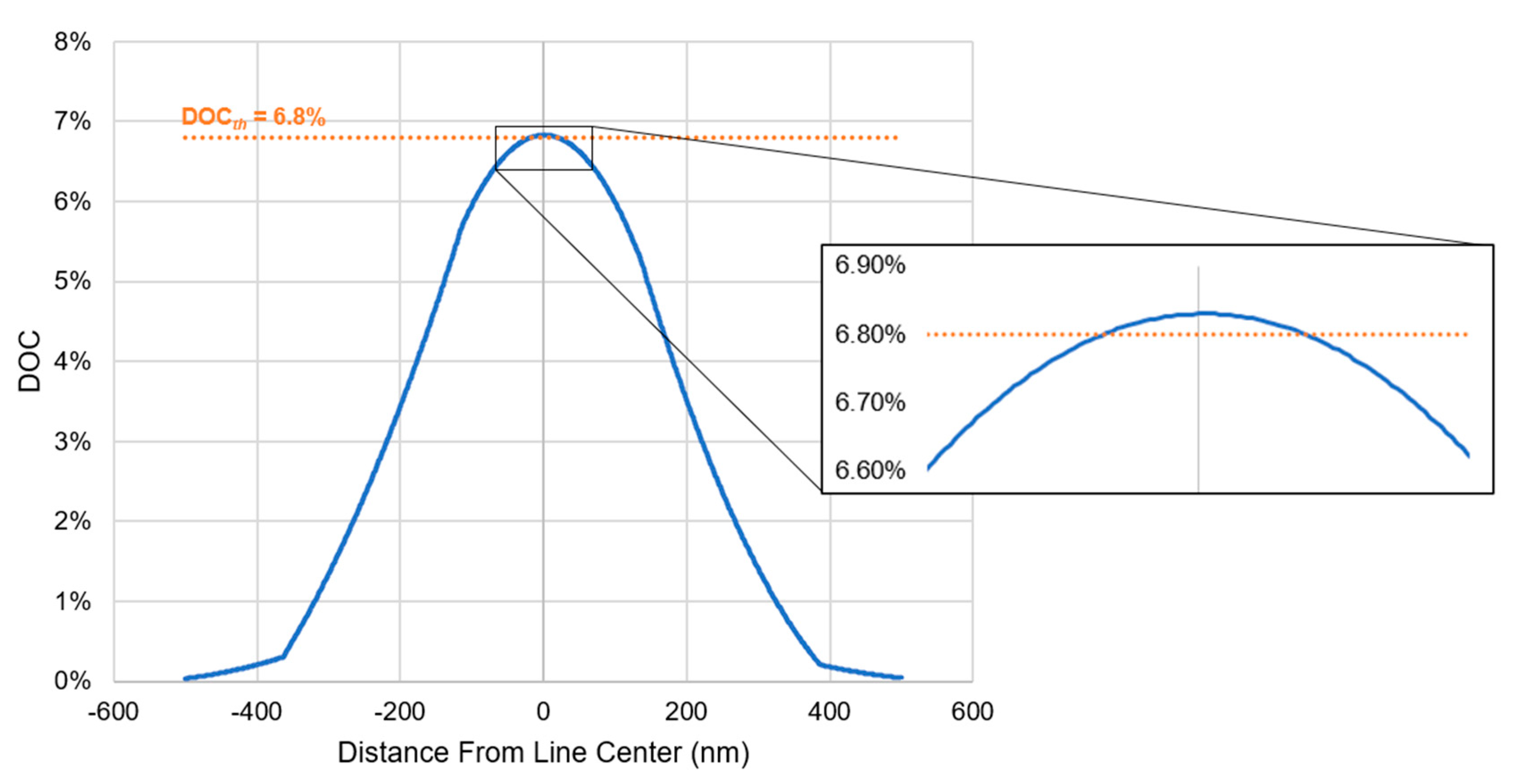
| DOCth | Degree of conversion threshold | 0.068 | Directly measured [35] |
| DO2 | Diffusivity of oxygen | 1.2 × 10⁻¹² m2 s–1 | Estimated using Stokes–Einstein (S-E) equation |
| DR* | Diffusivity of R* | 10−13 m2 s–1 | Estimated using S–E equation |
| v | Optical frequency (central) | 375 THz | Determined by laser in the printer |
| Parameter | List of Values |
|---|---|
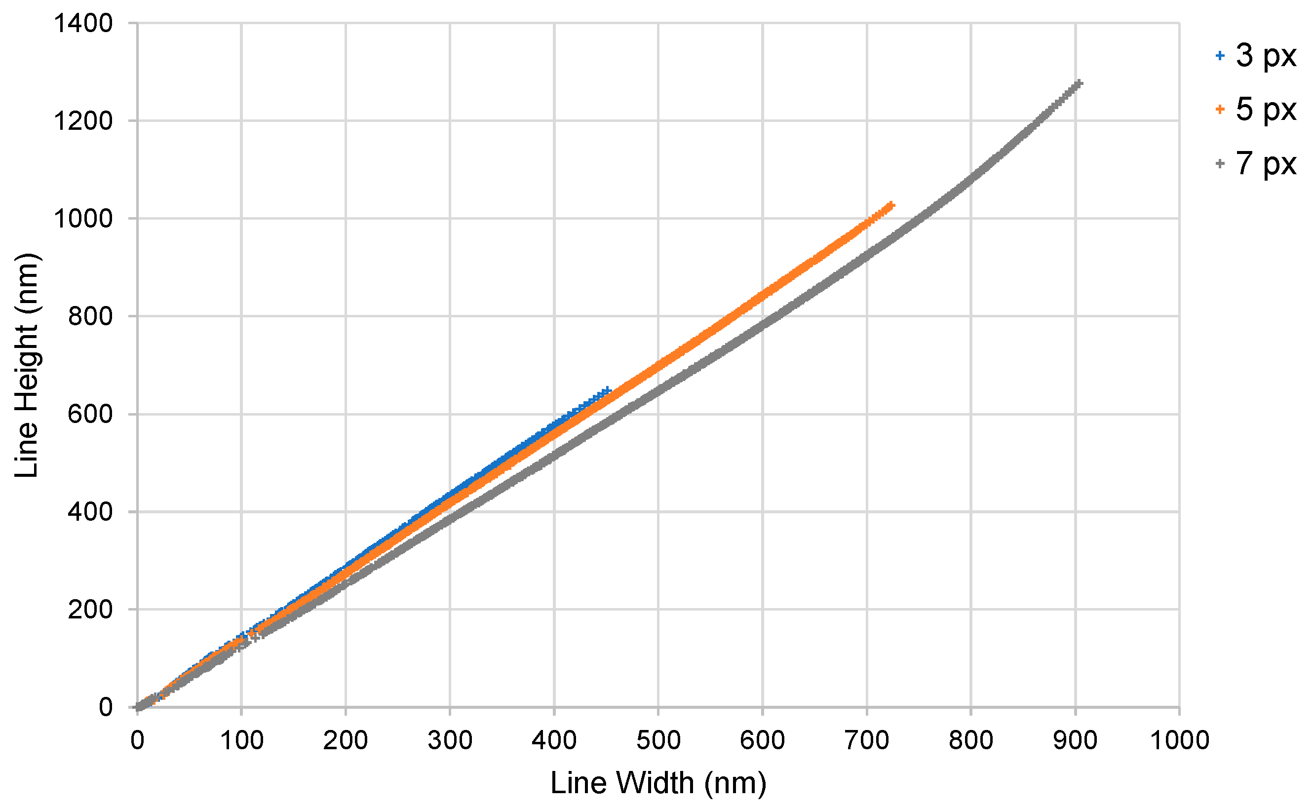
| Width of projected lines (px) | [3, 5, 7] |
| Exposure (number of pulses) | [2, 3, … 49, 50] |
| Average optical power of the beam (μW per px) | [0.01, 0.02, … 0.09, 0.10] × 1.56 |
| Photoinitiator concentration (mol m−3) | [0.25, 0.50, … 1.75, 2.00] |
Disclaimer/Publisher’s Note: The statements, opinions and data contained in all publications are solely those of the individual author(s) and contributor(s) and not of MDPI and/or the editor(s). MDPI and/or the editor(s) disclaim responsibility for any injury to people or property resulting from any ideas, methods, instructions or products referred to in the content. |
© 2024 by the authors. Licensee MDPI, Basel, Switzerland. This article is an open access article distributed under the terms and conditions of the Creative Commons Attribution (CC BY) license (https://creativecommons.org/licenses/by/4.0/).
Share and Cite
Pingali, R.; Kim, H.; Saha, S.K. A Computational Evaluation of Minimum Feature Size in Projection Two-Photon Lithography for Rapid Sub-100 nm Additive Manufacturing. Micromachines 2024, 15, 158. https://doi.org/10.3390/mi15010158
Pingali R, Kim H, Saha SK. A Computational Evaluation of Minimum Feature Size in Projection Two-Photon Lithography for Rapid Sub-100 nm Additive Manufacturing. Micromachines. 2024; 15(1):158. https://doi.org/10.3390/mi15010158
Chicago/Turabian StylePingali, Rushil, Harnjoo Kim, and Sourabh K. Saha. 2024. "A Computational Evaluation of Minimum Feature Size in Projection Two-Photon Lithography for Rapid Sub-100 nm Additive Manufacturing" Micromachines 15, no. 1: 158. https://doi.org/10.3390/mi15010158