
Experimental Study: The Effect of Pore Shape, Geometrical Heterogeneity, and Flow Rate on the Repetitive Two-Phase Fluid Transport in Microfluidic Porous Media


Abstract
:1. Introduction
2. Analysis Factors
2.1. Dimensionless Numbers
2.2. Correlation Coefficient
2.3. Minkowski Functionals
3. Review—Salient Flow Dynamics in Type I vs. Type II
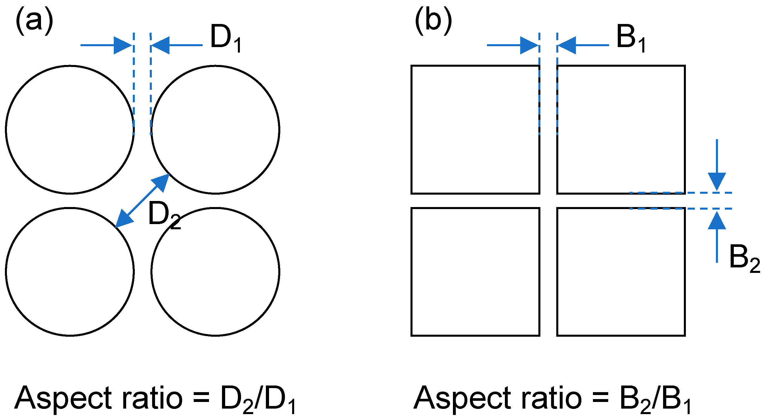
3.1. Pore Shape
3.2. Drainage
3.3. Imbibition
4. Experimental Study
4.1. Pore Structure of the Micromodel
4.2. Fabrication of the Pore-Network Micromodel
4.3. Materials
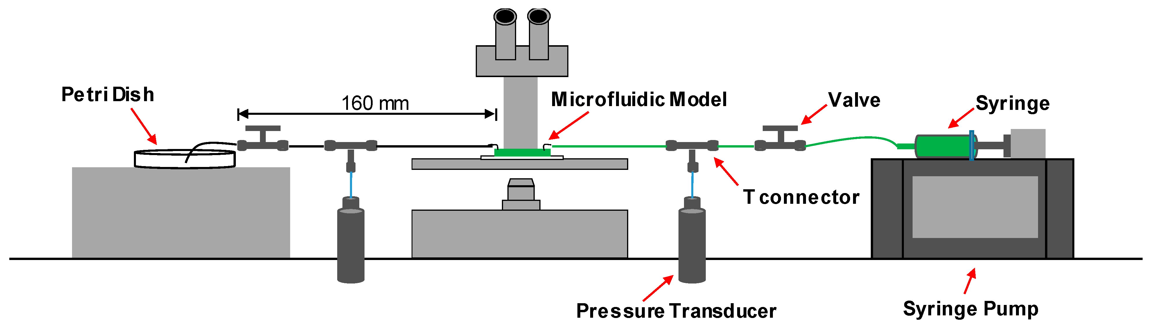
4.4. Experimental Setup and Procedure
5. Experimental Results and Analysis
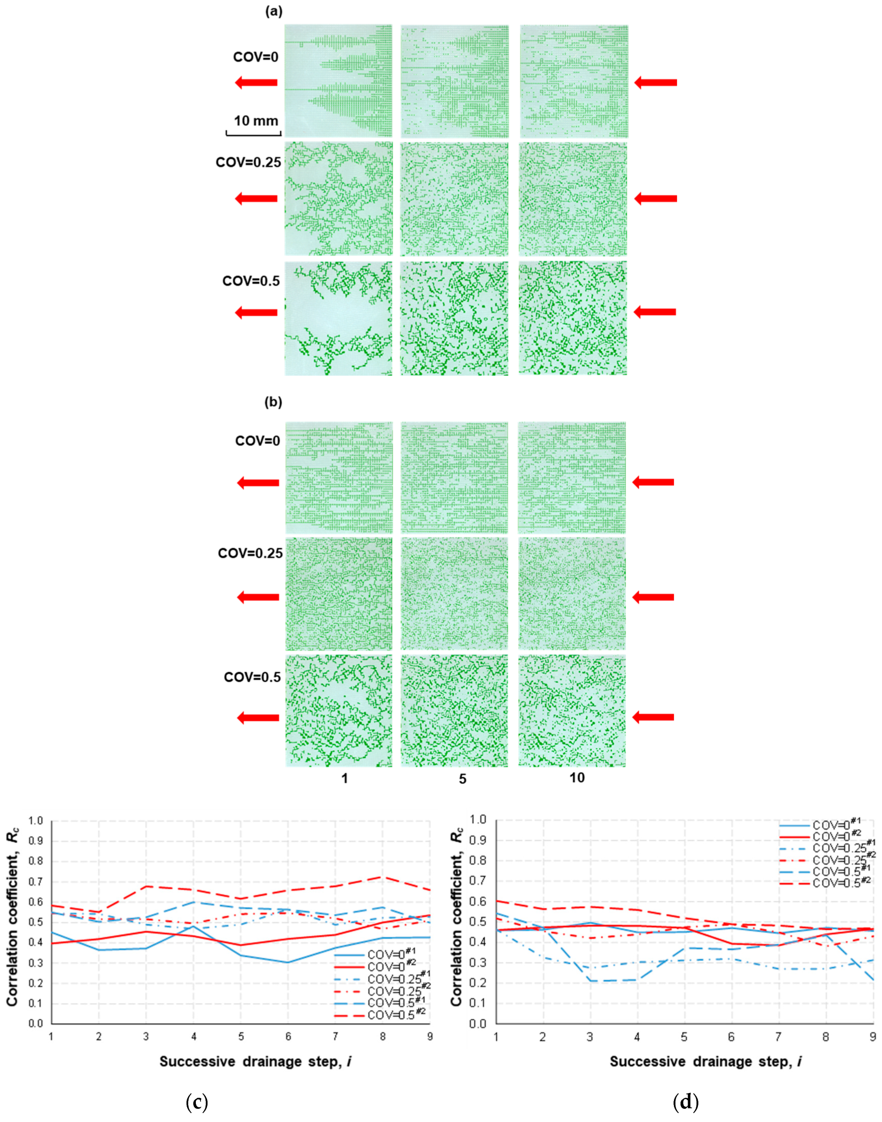
5.1. Drainages
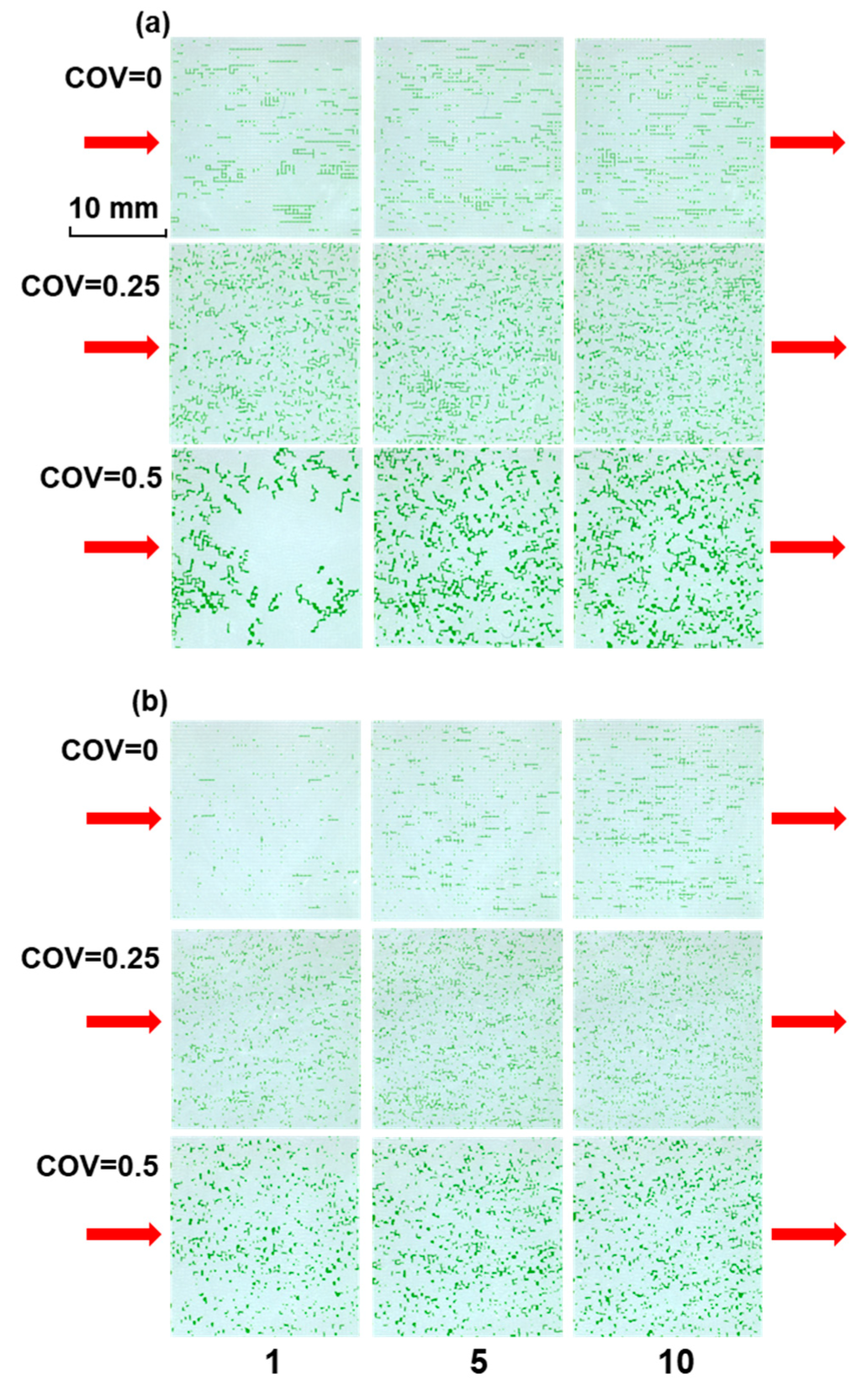
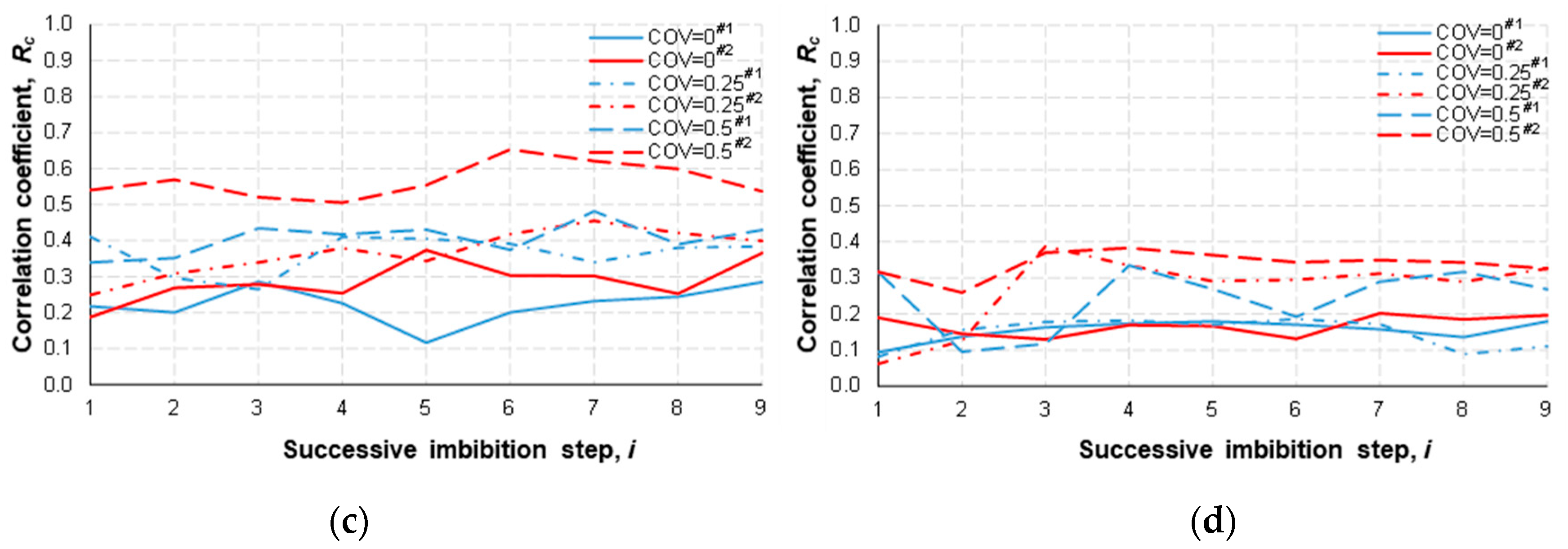
5.2. Imbibitions (Forced)
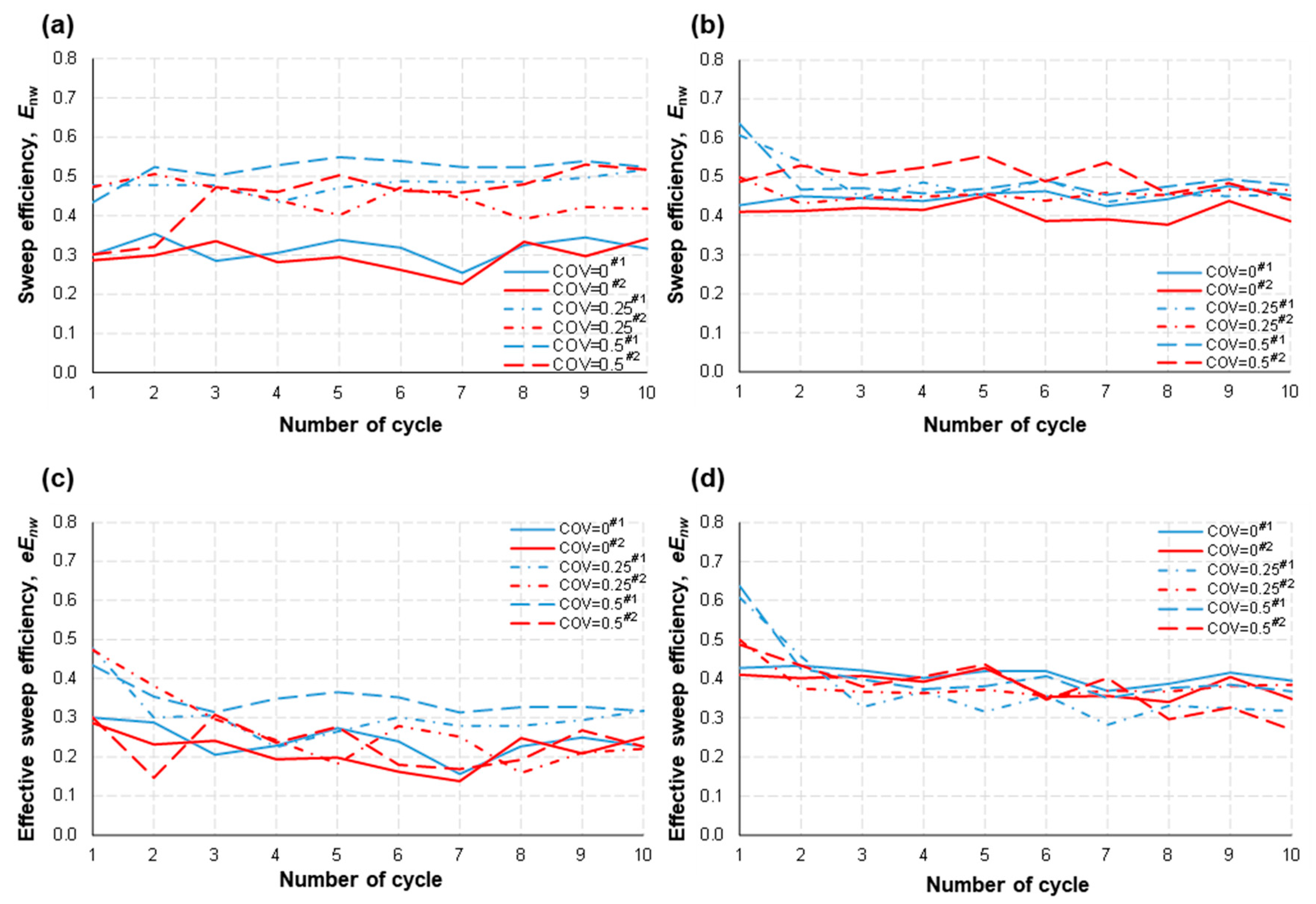
5.3. Sweep Efficiency
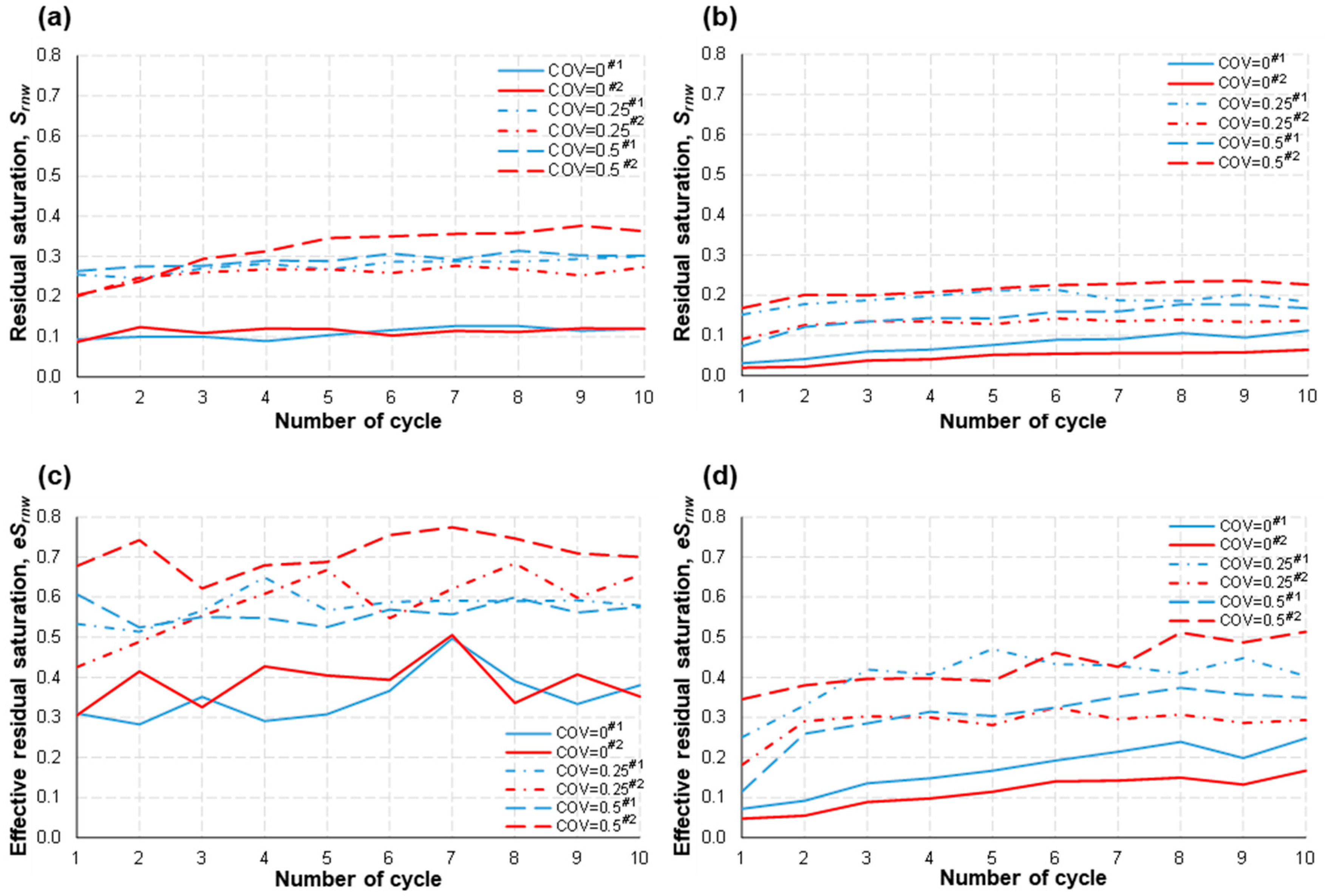
5.4. Residual Saturation
5.5. Flow Morphology
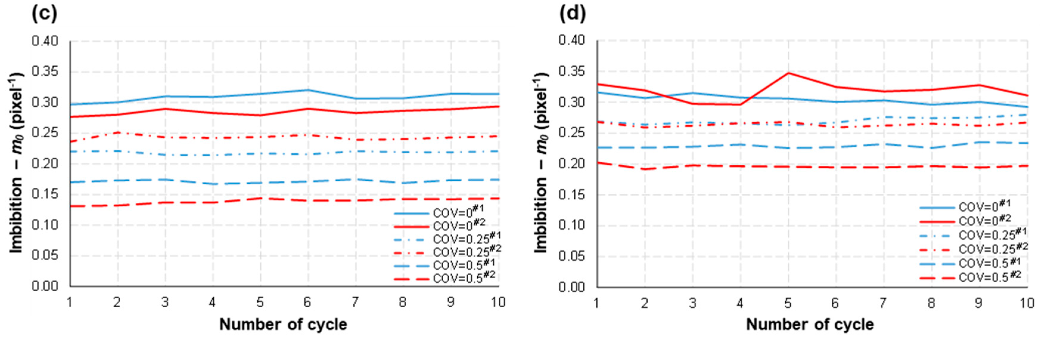
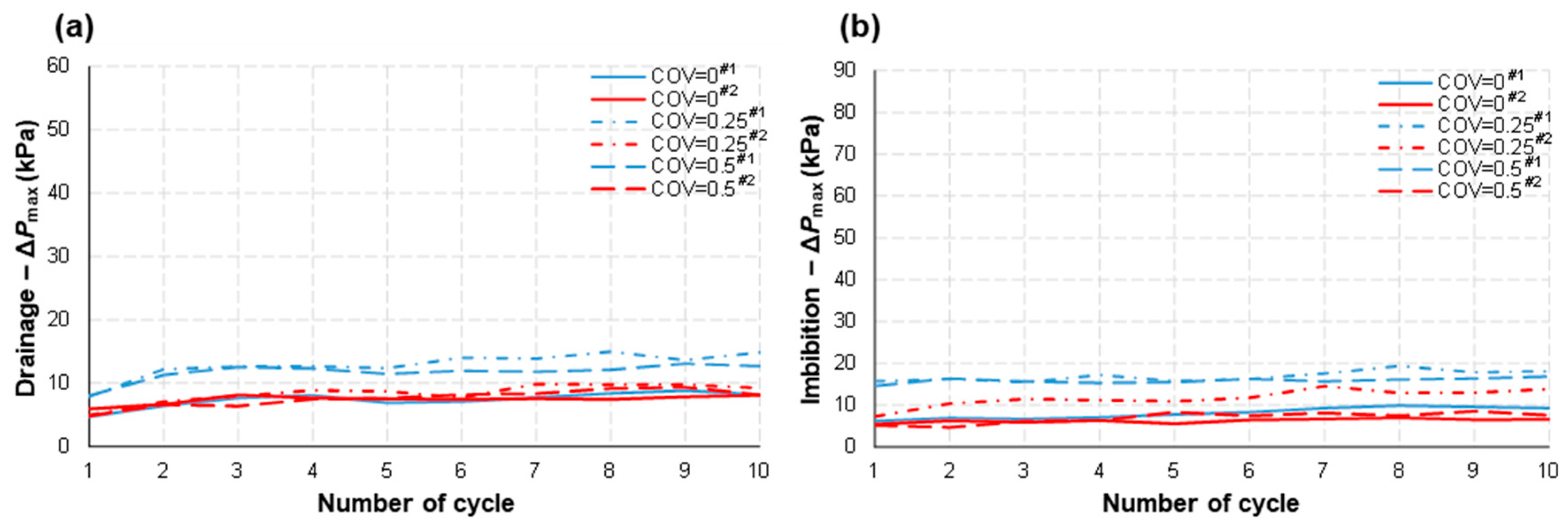
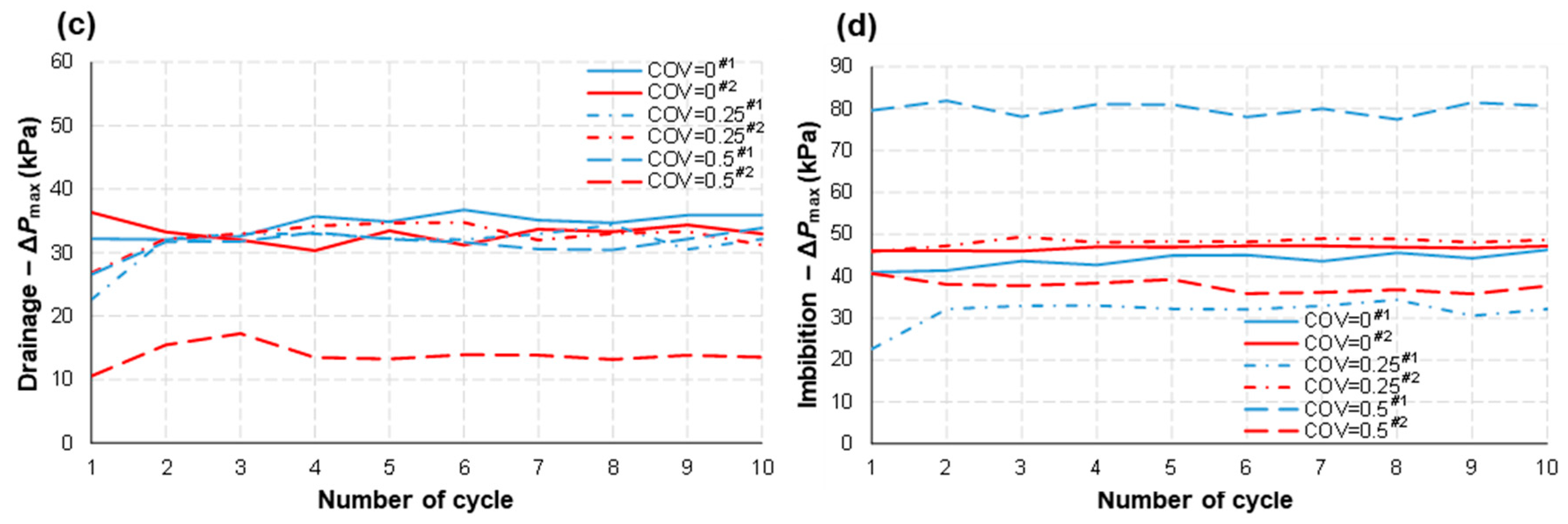
5.6. Fluid Pressure
6. Discussion
6.1. Impact of COV (Pore-Space Heterogeneity), Q (Flow Rate), and Aspect Ratio (Pore Shape)
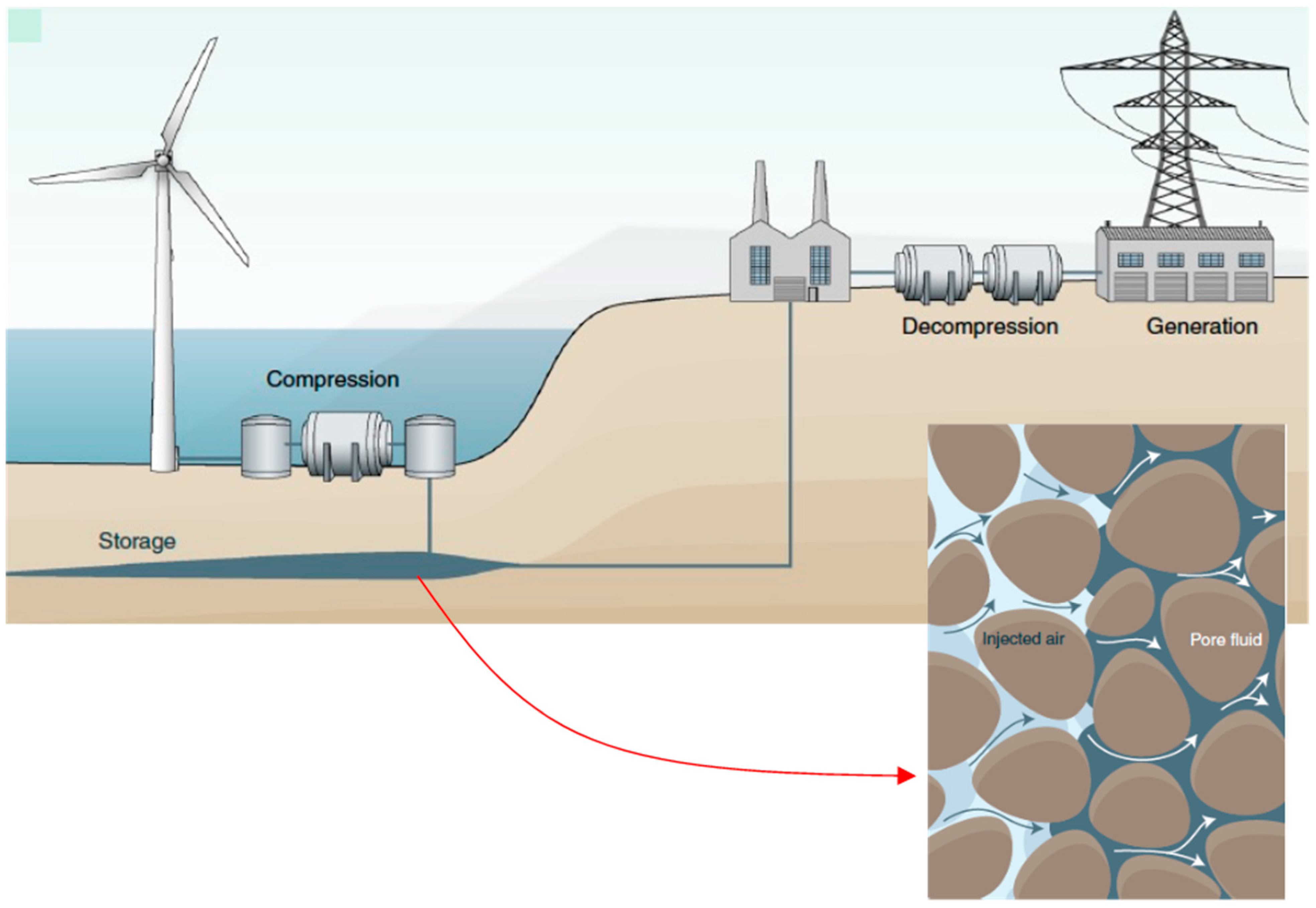
6.2. Implications for Air/Gas Storage
7. Conclusions
Author Contributions
Funding
Data Availability Statement
Acknowledgments
Conflicts of Interest
References
- Mongird, K.; Viswanathan, V.; Alam, J.; Vartanian, C.; Sprenkle, V.; Baxter, R. 2020 grid energy storage technology cost and performance assessment. Energy 2020, 2020, 6–15. [Google Scholar]
- Kim, S.; Dusseault, M.; Babarinde, O.; Wickens, J. Compressed air energy storage (CAES): Current status, geomechanical aspects and future opportunities. Geol. Soc. Lond. Spec. Publ. 2023, 528, SP528-2022. [Google Scholar] [CrossRef]
- Zhang, J.; Zhang, H.; Lee, D.; Ryu, S.; Kim, S. Study on the effect of pore-scale heterogeneity and flow rate during repetitive two-phase fluid flow in microfluidic porous media. Pet. Geosci. 2021, 27, petgeo2020-062. [Google Scholar] [CrossRef]
- Bentham, M. A porous medium for all seasons. Nat. Energy 2019, 4, 97–98. [Google Scholar] [CrossRef]
- Zhang, J.; Zhang, H.; Lee, D.; Ryu, S.; Kim, S. Microfluidic Study on the Two-Phase Fluid Flow in Porous Media During Repetitive Drainage-Imbibition Cycles and Implications to the CAES Operation. Transp. Porous Media 2020, 131, 449–472. [Google Scholar] [CrossRef]
- Lenormand, R.; Touboul, E.; Zarcone, C. Numerical models and experiments on immiscible displacements in porous media. J. Fluid Mech. 1988, 189, 165–187. [Google Scholar] [CrossRef]
- Avraam, D.G.; Payatakes, A.C. Flow regimes and relative permeabilities during steady-state two-phase flow in porous media. J. Fluid Mech. 1995, 293, 207–236. [Google Scholar] [CrossRef]
- Mantz, H.; Jacobs, K.; Mecke, K. Utilizing Minkowski functionals for image analysis: A marching square algorithm. J. Stat. Mech. Theory Exp. 2008, 2008, P12015. [Google Scholar] [CrossRef]
- Schluter, S.; Berg, S.; Rucker, M.; Armstrong, R.T.; Vogel, H.J.; Hilfer, R.; Wildenschild, D. Pore-scale displacement mechanisms as a source of hysteresis for two-phase flow in porous media. Water Resour. Res. 2016, 52, 2194–2205. [Google Scholar] [CrossRef] [Green Version]
- Jambayev, A.S. Discrete Fracture Network Modeling for a Carbonate Reservoir; Colorado School of Mines: Golden, CO, USA, 2013. [Google Scholar]
- Bear, J. Dynamics of Fluids in Porous Media; Courier Corporation: Chelmsford, MA, USA, 2013. [Google Scholar]
- Follesø, H.N. Fluid Displacements during Multiphase Flow Visualized at the Pore Scale Using Micromodels. Master’s Thesis, University of Bergen, Bergen, Norway, 2012. [Google Scholar]
- Nelson, P.H. Pore-throat sizes in sandstones, tight sandstones, and shales. AAPG Bull. 2009, 93, 329–340. [Google Scholar] [CrossRef]
- Warren, J.E.; Root, P.J. The behavior of naturally fractured reservoirs. Soc. Pet. Eng. J. 1963, 3, 245–255. [Google Scholar] [CrossRef] [Green Version]
- Soleimani, M. Naturally fractured hydrocarbon reservoir simulation by elastic fracture modeling. Pet. Sci. 2017, 14, 286–301. [Google Scholar] [CrossRef] [Green Version]
- Lenormand, R. Liquids in porous media. J. Phys. Condens. Matter 1990, 2, SA79. [Google Scholar] [CrossRef]
- Lenormand, R.; Zarcone, C.; Sarr, A. Mechanisms of the displacement of one fluid by another in a network of capillary ducts. J. Fluid Mech. 1983, 135, 337–353. [Google Scholar] [CrossRef] [Green Version]
- Vizika, O. Parametric experimental study of forced imbibition in porous media. Phys. Chem. Hydrodyn. 1989, 11, 187–204. [Google Scholar]
- Lenormand, R.; Zarcone, C. Role of roughness and edges during imbibition in square capillaries. In SPE Annual Technical Conference and Exhibition; Society of Petroleum Engineers: Richardson, TX, USA, 1984. [Google Scholar] [CrossRef]
- Andrew, M.; Bijeljic, B.; Blunt, M.J. Pore-by-pore capillary pressure measurements using X-ray microtomography at reservoir conditions: Curvature, snap-off, and remobilization of redidual CO2. Water Resour. Res. 2014, 50, 8760–8774. [Google Scholar] [CrossRef] [Green Version]
- Delamarche, E.; Schmid, H.; Michel, B.; Biebuyck, H. Stability of molded polydimethylsiloxane microstructures. Adv. Mater. 1997, 9, 741–746. [Google Scholar] [CrossRef]
- Xia, Y.; Whitesides, G.M. Soft lithography. Annu. Rev. Mater. Sci. 1998, 28, 153–184. [Google Scholar] [CrossRef]
- Zheng, X.; Mahabadi, N.; Sup Yun, T.; Jang, J. Effect of capillary and viscous force on CO2 saturation and invasion pattern in the microfluidic chip. J. Geophys. Res. Solid Earth 2017, 122, 1634–1647. [Google Scholar] [CrossRef]
- Guo, C.; Zhang, K.; Pan, L.; Cai, Z.; Li, C.; Li, Y. Numerical investigation of a joint approach to thermal energy storage and compressed air energy storage in aquifers. Appl. Energy 2017, 203, 948–958. [Google Scholar] [CrossRef] [Green Version]
- Guo, C.; Zhang, K.; Li, C.; Wang, X. Modelling studies for influence factors of gas bubble in compressed air energy storage in aquifers. Energy 2016, 107, 48–59. [Google Scholar] [CrossRef]
- Oldenburg, C.M.; Pan, L. Porous Media Compressed-Air Energy Storage (PM-CAES): Theory and Simulation of the Coupled Wellbore-Reservoir System. Transp. Porous Media 2013, 97, 201–221. [Google Scholar] [CrossRef] [Green Version]
- Wiles, L.E.; McCann, R.A. Water Coning in Porous Media Reservoirs for Compressed Air Energy Storage (No. PNL-3470); Battelle Pacific Northwest Labs: Richland, WA, USA, 1981. [Google Scholar]


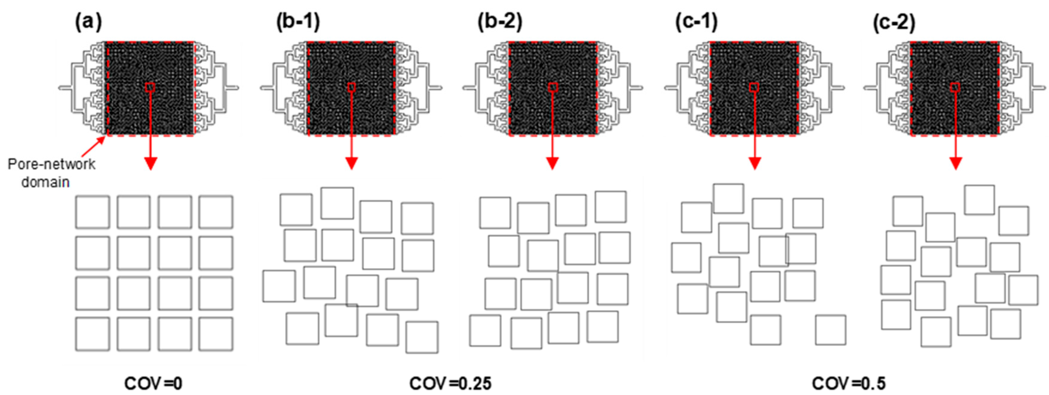
| Parameters | Figure 3b-1 | Figure 3b-2 | Figure 3c-1 | Figure 3c-2 |
|---|---|---|---|---|
| COV = σw/w | 0.25 | 0.25 | 0.5 | 0.5 |
| Mean width, w (μm) | 80 | 80 | 80 | 80 |
| Standard deviation, σw (μm) | 20 | 20 | 40 | 40 |
| Minimum width, wmin (μm) | 20 | 20 | 20 | 20 |
| Height, h (μm) | 100 | 100 | 100 | 100 |
| Effective porosity | 0.36 | 0.36 | 0.38 | 0.38 |
| Permeability (Darcy) | 4.2 | 5.9 | 4.0 | 6.4 |
| Mineral Oil * | Water | Water–Oil | ||
|---|---|---|---|---|
| Viscosity (Pa·s) | Density (kg/m3) | Viscosity (Pa·s) | Density (kg/m3) | Interfacial Tension (mN/m) |
| 4.2 × 10⁻² | 830 | 1.0 × 10⁻³ | 1000 | 52 |
| Q | 0.01 mL/min | 0.1 mL/min | ||||
|---|---|---|---|---|---|---|
| COV | 0 | 0.25 | 0.5 | 0 | 0.25 | 0.5 |
| Rc—Drainage | 0.3–0.55 | 0.45–0.55 | 0.5–0.7 | 0.4–0.5 | 0.25–0.5 | 0.2–0.6 |
| Rc—Imbibition | 0.1–0.35 | 0.25–0.45 | 0.35–0.65 | 0.1–0.2 | 0.1–0.4 | 0.1–0.4 |
| Enw | 0.25–0.35 | 0.4–0.5 | 0.3–0.55 | 0.35–0.45 | 0.45–0.6 | 0.45–0.55 |
| eEnw * | 0.15–0.3 | 0.15–0.4 | 0.15–0.35 | 0.35–0.45 | 0.3–0.45 | 0.3–0.45 |
| Srnw | 0.1–0.15 | 0.25–0.3 | 0.2–0.35 | 0.05–0.1 | 0.1–0.2 | 0.1–0.25 |
| eSrnw * | 0.3–0.5 | 0.5–0.7 | 0.55–0.8 | 0.05–0.25 | 0.3–0.45 | 0.25–0.5 |
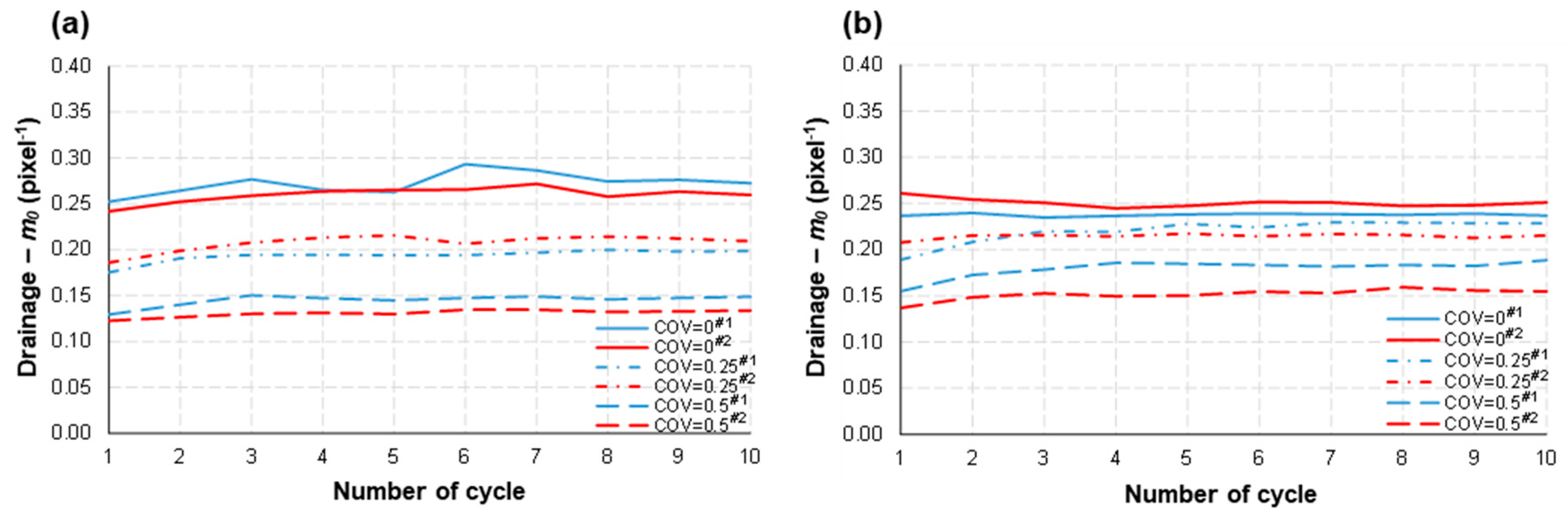
| m0—Drainage | 0.25–0.3 | 0.17–0.25 | 0.13–0.15 | 0.24–0.25 | 0.22–0.23 | 0.15–0.18 |
| m0—Imbibition | 0.28–0.32 | 0.22–0.25 | 0.14–0.17 | 0.3–0.35 | 0.26–0.27 | 0.2–0.23 |
| ΔPmax—Drainage | 5–8 kPa | 5–15 kPa | 5–14 kPa | 30–35 kPa | 22–35 kPa | 10–33 kPa |
| ΔPmax—Imbibition | 6–10 kPa | 8–20 kPa | 5–15 kPa | 40–47 kPa | 25–50 kPa | 35–80 kPa |
Disclaimer/Publisher’s Note: The statements, opinions and data contained in all publications are solely those of the individual author(s) and contributor(s) and not of MDPI and/or the editor(s). MDPI and/or the editor(s) disclaim responsibility for any injury to people or property resulting from any ideas, methods, instructions or products referred to in the content. |
© 2023 by the authors. Licensee MDPI, Basel, Switzerland. This article is an open access article distributed under the terms and conditions of the Creative Commons Attribution (CC BY) license (https://creativecommons.org/licenses/by/4.0/).
Share and Cite
Kim, S.; Zhang, J.; Ryu, S. Experimental Study: The Effect of Pore Shape, Geometrical Heterogeneity, and Flow Rate on the Repetitive Two-Phase Fluid Transport in Microfluidic Porous Media. Micromachines 2023, 14, 1441. https://doi.org/10.3390/mi14071441
Kim S, Zhang J, Ryu S. Experimental Study: The Effect of Pore Shape, Geometrical Heterogeneity, and Flow Rate on the Repetitive Two-Phase Fluid Transport in Microfluidic Porous Media. Micromachines. 2023; 14(7):1441. https://doi.org/10.3390/mi14071441
Chicago/Turabian StyleKim, Seunghee, Jingtao Zhang, and Sangjin Ryu. 2023. "Experimental Study: The Effect of Pore Shape, Geometrical Heterogeneity, and Flow Rate on the Repetitive Two-Phase Fluid Transport in Microfluidic Porous Media" Micromachines 14, no. 7: 1441. https://doi.org/10.3390/mi14071441