
Spin Hall Effect in the Paraxial Light Beams with Multiple Polarization Singularities

Abstract
:1. Introduction
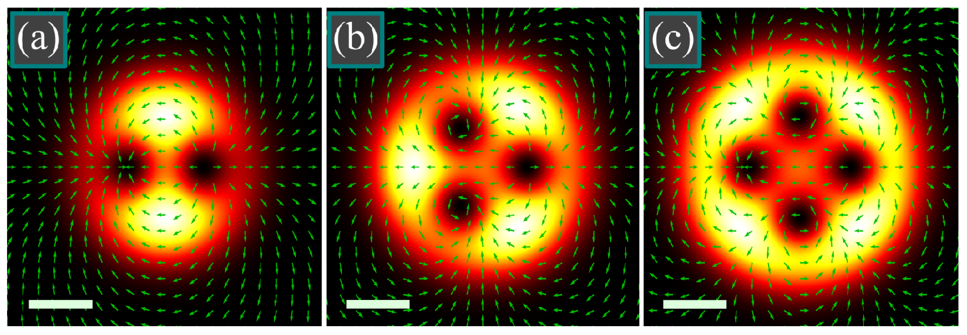
2. Paraxial Light Fields with Multiple Phase or Polarization Singularities
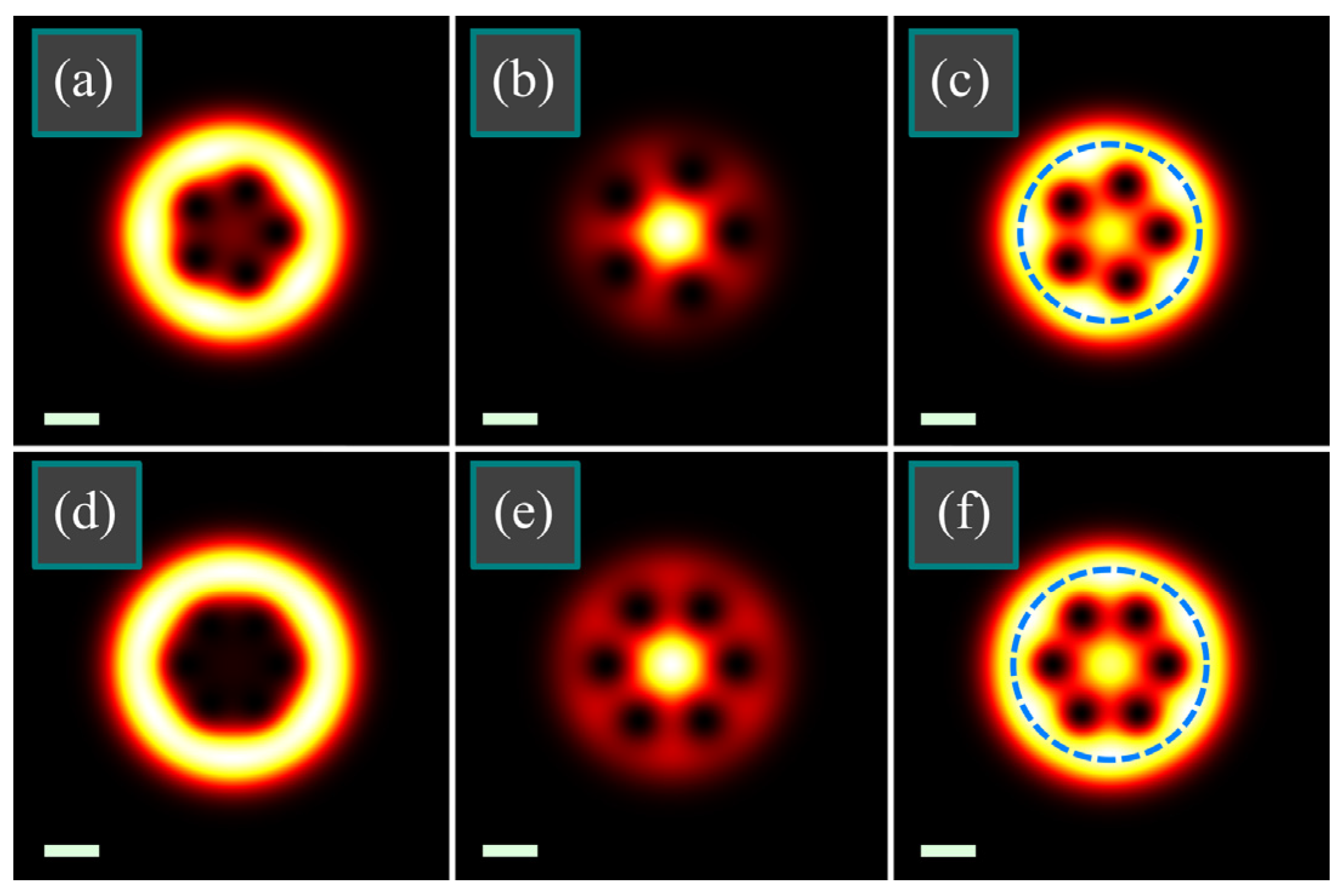
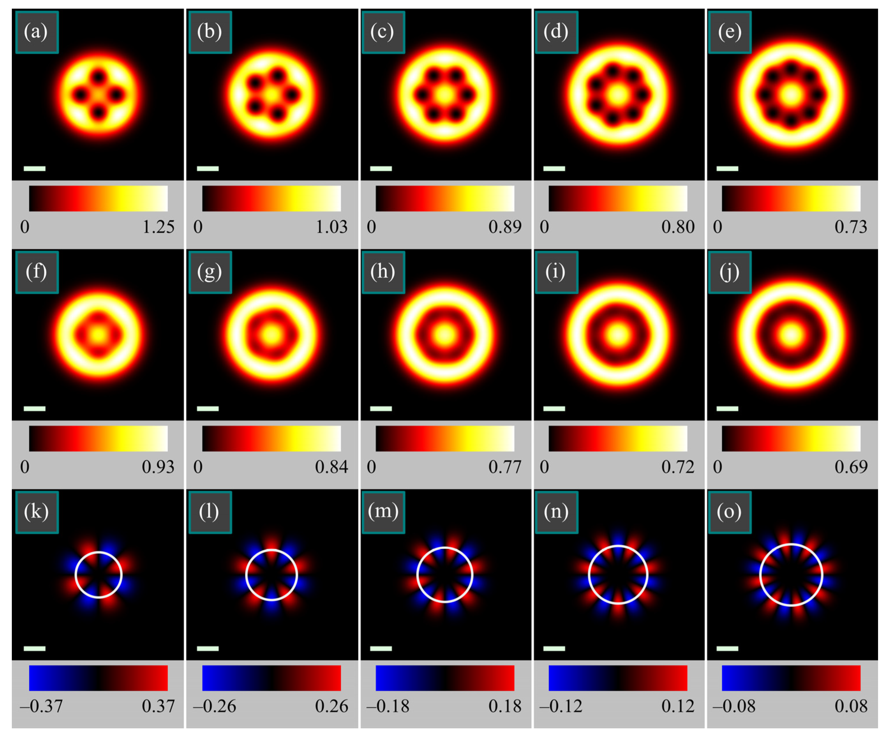
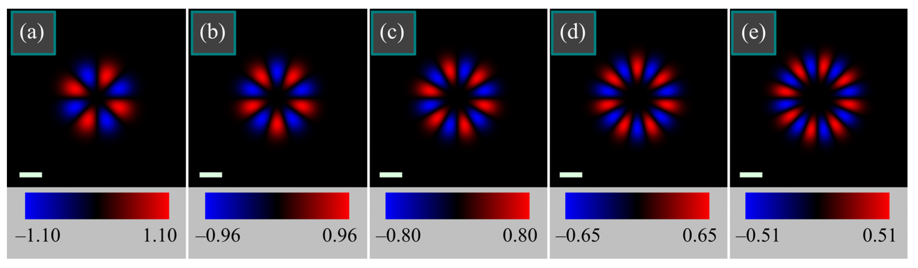
3. Intensity Distribution
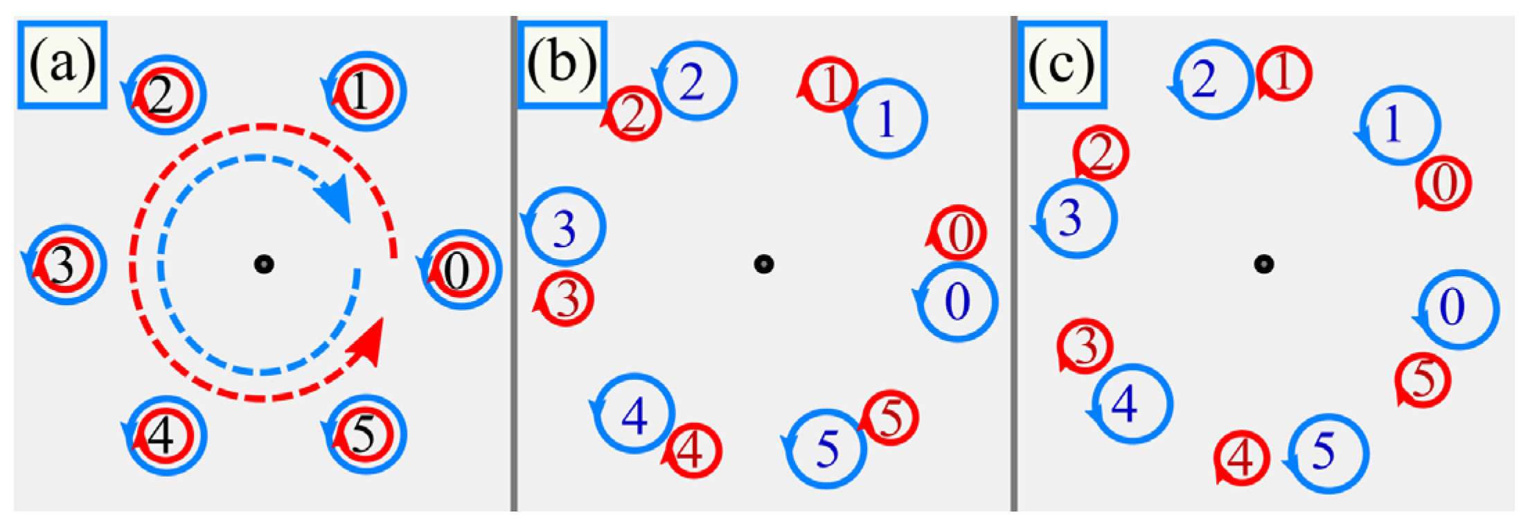
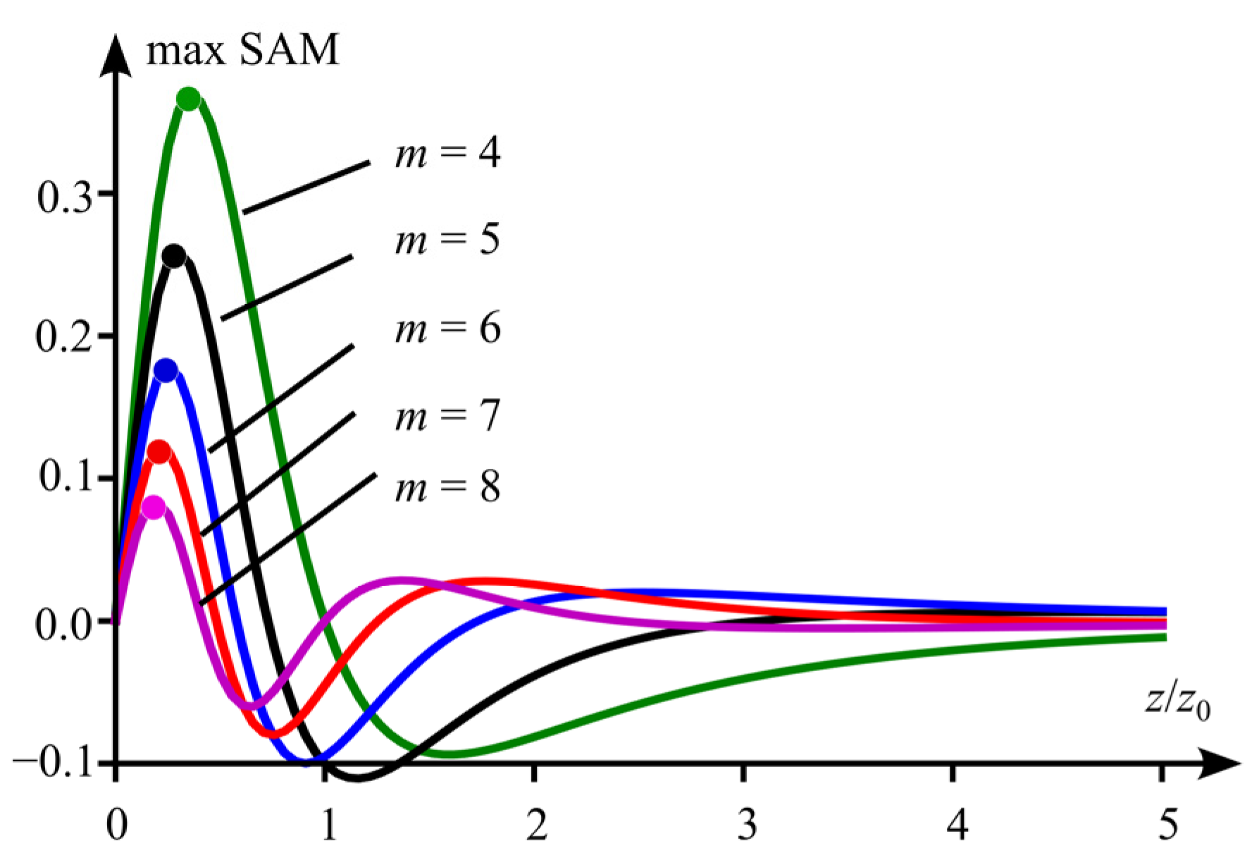
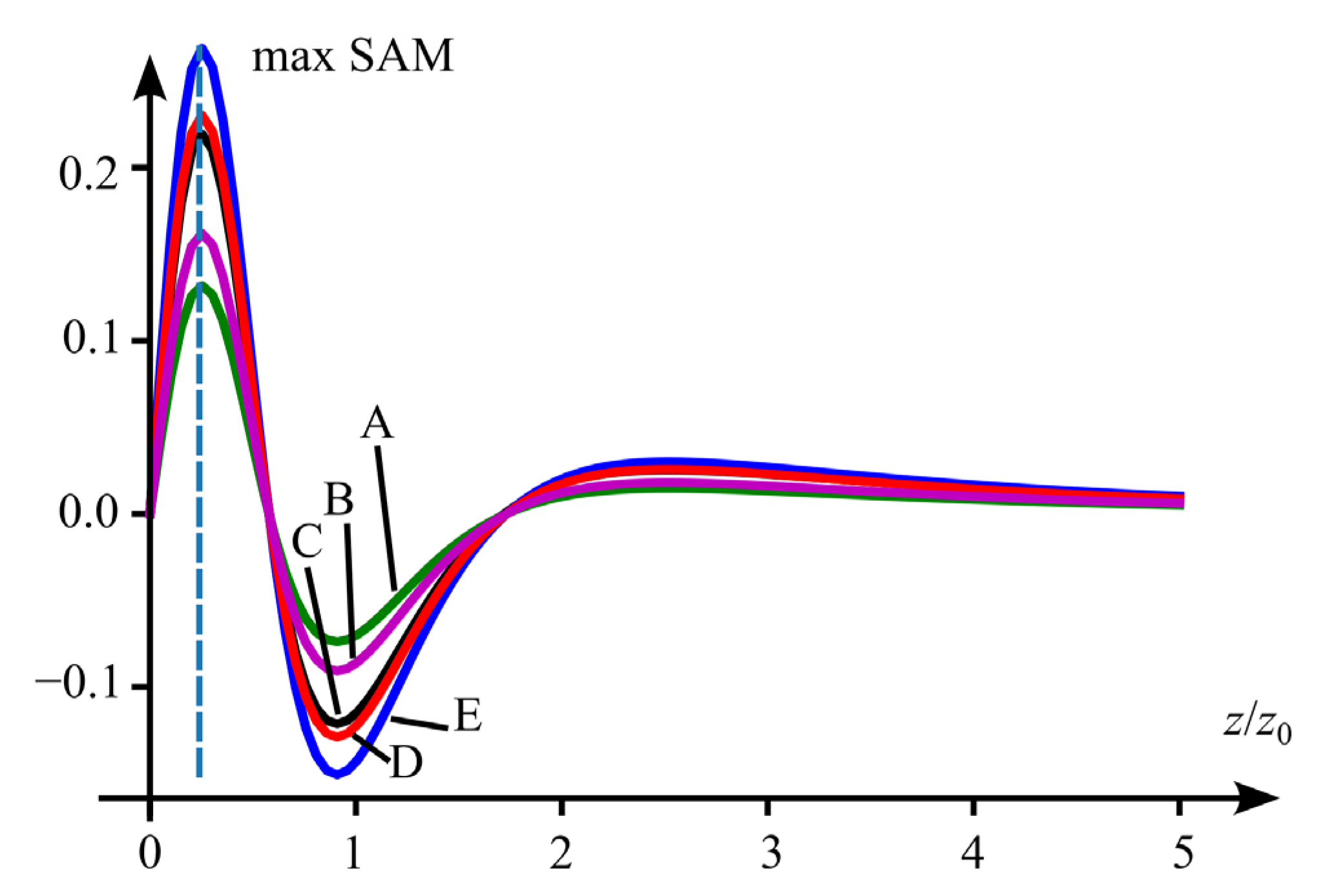
4. Spin Angular Momentum Density
5. Orbital Angular Momentum Density
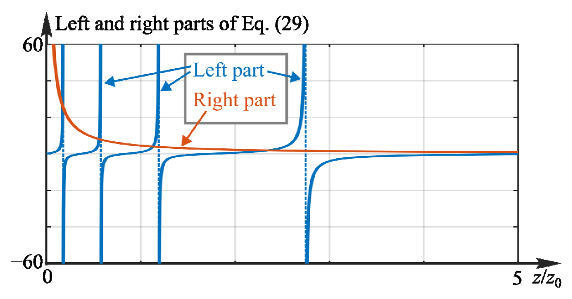
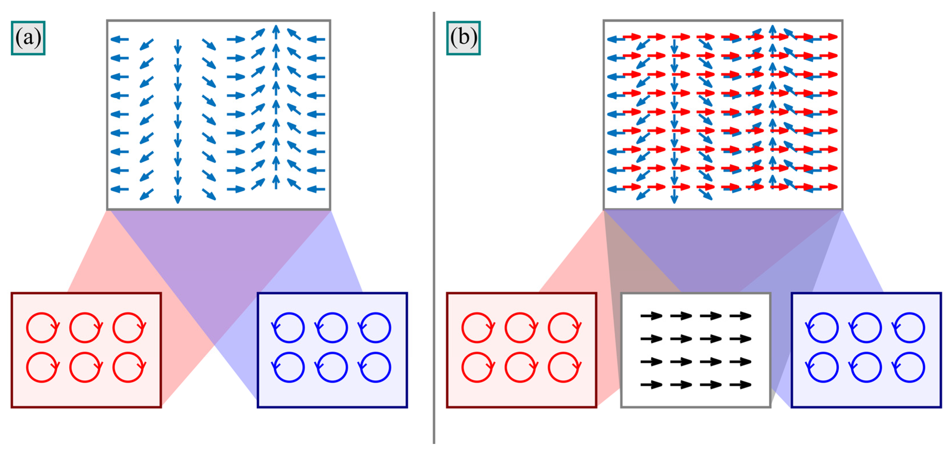
6. Analogy with Plane Wave and Revealing the Mechanism
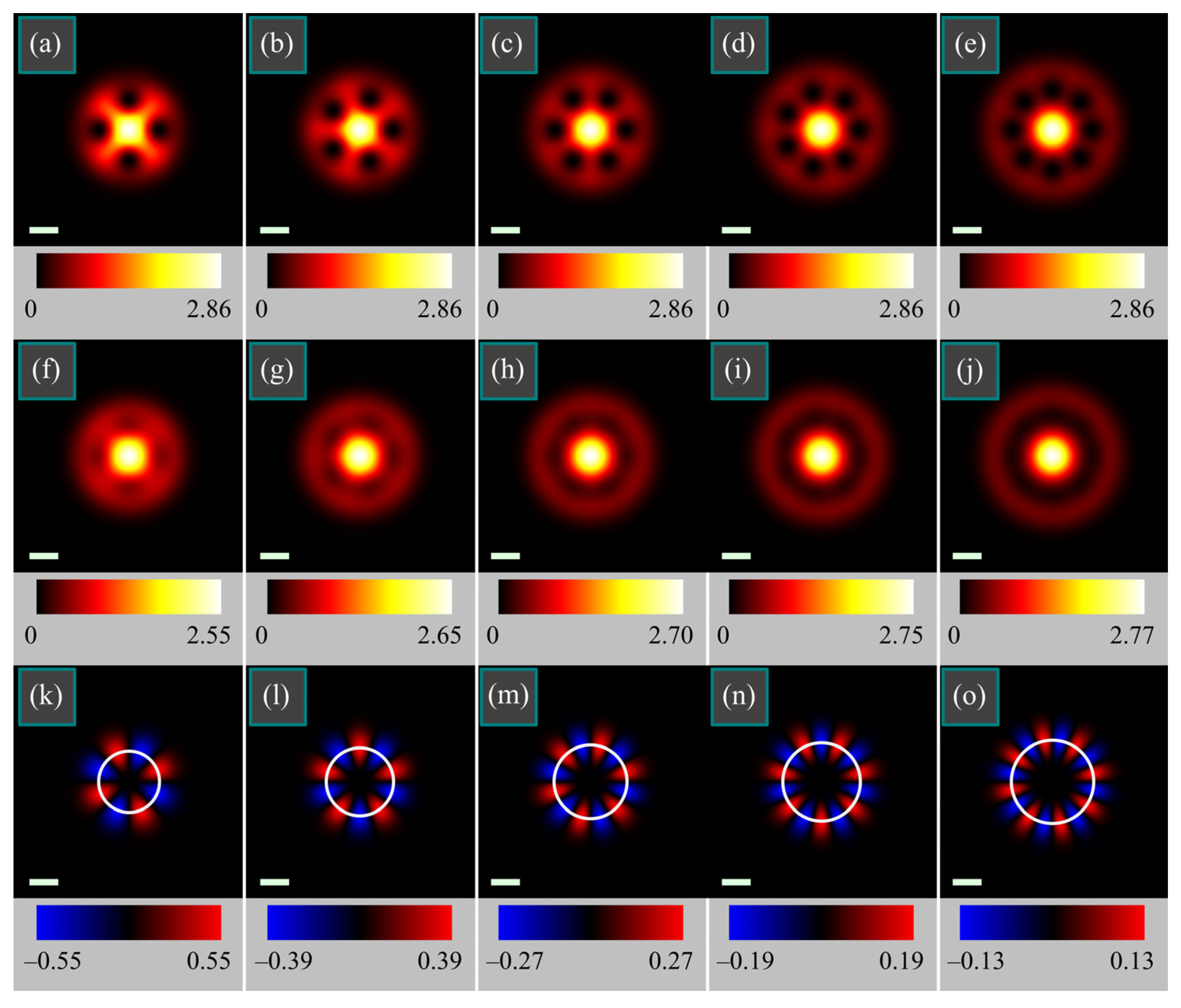
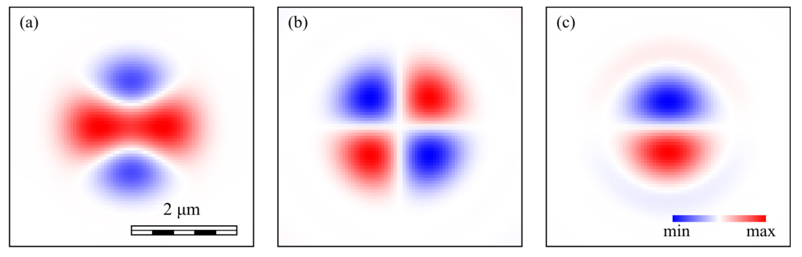
7. Simulation
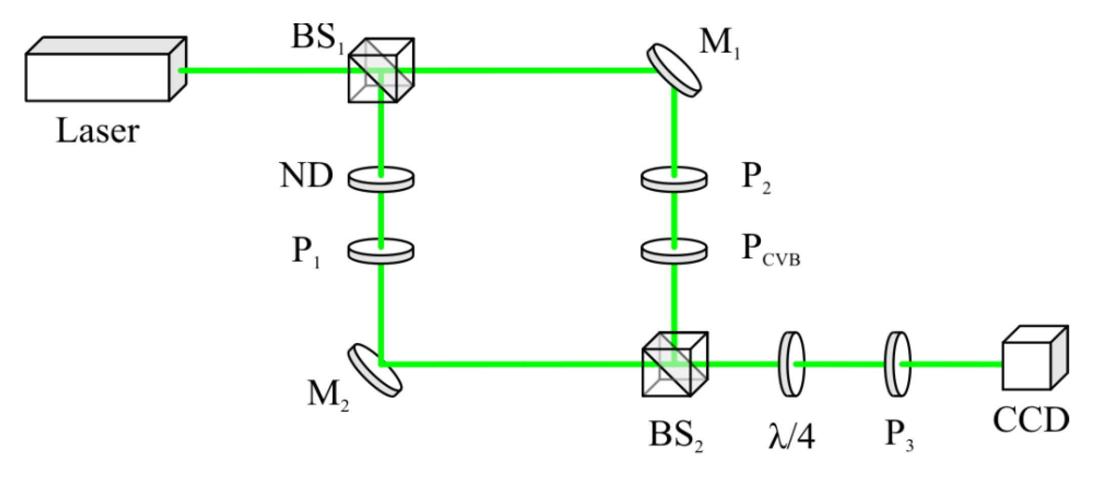
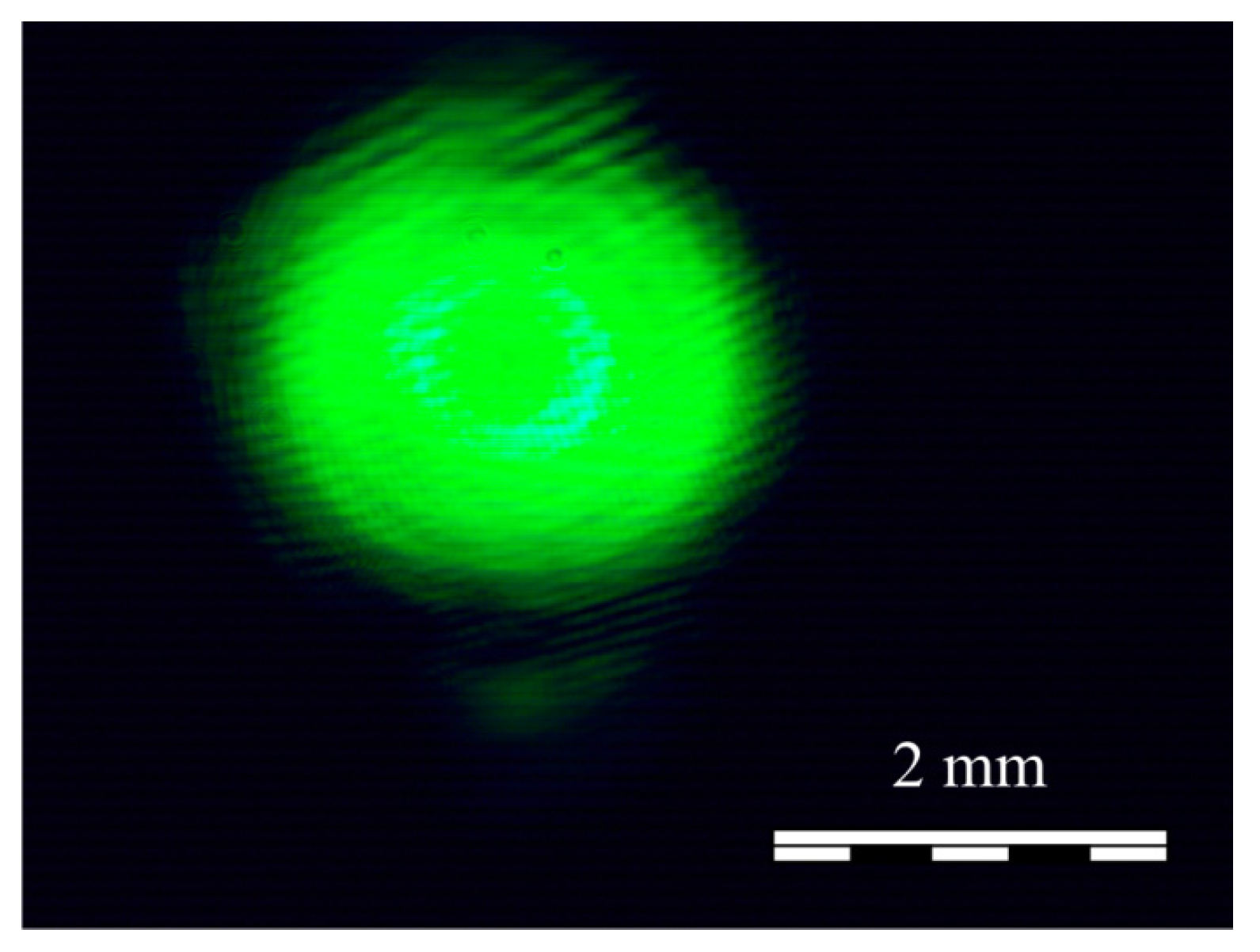
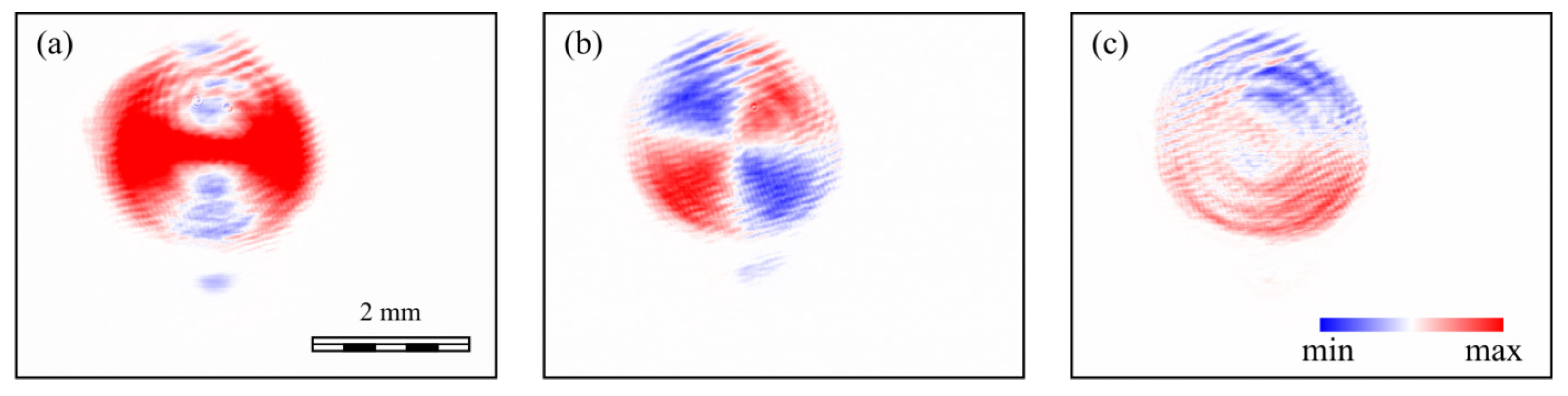
8. Experiment
9. Conclusions
Author Contributions
Funding
Data Availability Statement
Conflicts of Interest
References
- Indebetouw, G. Optical Vortices and Their Propagation. J. Mod. Opt. 1993, 40, 73–87. [Google Scholar] [CrossRef]
- Abramochkin, E.G.; Volostnikov, V.G. Spiral-type beams. Opt. Commun. 1993, 102, 336. [Google Scholar] [CrossRef]
- Wang, Q.; Tu, C.H.; Li, Y.N.; Wang, H.T. Polarization singularities: Progress, fundamental physics, and prospects. APL Photonics 2021, 6, 040901. [Google Scholar] [CrossRef]
- Zhan, Q. Cylindrical vector beams: From mathematical concepts to applications. Adv. Opt. Photon. 2009, 1, 1–57. [Google Scholar] [CrossRef]
- Tidwell, S.C.; Ford, D.H.; Kimura, W.D. Generating radially polarized beams interferometrically. Appl. Opt. 1990, 29, 2234–2239. [Google Scholar] [CrossRef] [PubMed]
- Kovalev, A.A.; Kotlyar, V.V. Tailoring polarization singularities in a Gaussian beam with locally linear polarization. Opt. Lett. 2018, 43, 3084–3087. [Google Scholar] [CrossRef]
- Kovalev, A.A.; Kotlyar, V.V. Gaussian beams with multiple polarization singularities. Opt. Commun. 2018, 423, 111–120. [Google Scholar] [CrossRef]
- Wang, H.; Wojcik, C.C.; Fan, S. Topological spin defects of light. Optica 2022, 9, 1417–1423. [Google Scholar] [CrossRef]
- Dyakonov, M.I.; Perel, V.I. Current-induced spin orientation of electrons in semiconductors. Phys. Lett. A 1971, 35, 459–460. [Google Scholar] [CrossRef]
- Onoda, M.; Murakami, S.; Nagaosa, N. Hall effect of light. Phys. Rev. Lett. 2004, 93, 083901. [Google Scholar] [CrossRef] [Green Version]
- Liu, S.Q.; Chen, S.Z.; Wen, S.C.; Luo, H.L. Photonic spin Hall effect: Fundamentals and emergent applications. Opto-Electron. Sci. 2022, 1, 220007. [Google Scholar] [CrossRef]
- Liu, S.; Qi, S.; Li, Y.; Wei, B.; Li, P.; Zhao, J. Controllable oscillated spin Hall effect of Bessel beam realized by liquid crystal Pancharatnam-Berry phase elements. Light Sci. Appl. 2022, 11, 219. [Google Scholar] [CrossRef] [PubMed]
- Leyder, C.; Romanelli, M.; Karr, J.P.; Giacobino, E.; Liew, T.C.; Glazov, M.M.; Kavokin, A.V.; Malpuech, G.; Bramati, A. Observation of the optical spin Hall effect. Nat. Phys. 2007, 3, 628–631. [Google Scholar] [CrossRef]
- Zhang, J.; Zhou, X.X.; Ling, X.H.; Chen, S.Z.; Luo, H.L.; Wen, S.C. Orbit-orbit interaction and photonic orbital Hall effect in reflection of a light beam. Chin. Phys. B 2014, 23, 064215. [Google Scholar] [CrossRef]
- He, Y.; Xie, Z.; Yang, B.; Chen, X.; Liu, J.; Ye, H.; Zhou, X.X.; Li, Y.; Chen, S.Q.; Fan, D. Controllable photonic spin Hall effect with phase function construction. Photonics Res. 2020, 8, 963–971. [Google Scholar] [CrossRef]
- Bliokh, K.Y.; Bliokh, Y.P. Conservation of angular momentum, transverse shift, and spin Hall effect in reflection and refraction of an electromagnetic wave packet. Phys. Rev. Lett. 2006, 96, 073903. [Google Scholar] [CrossRef] [Green Version]
- Kavokin, A.; Malpuech, G.; Glazov, M. Optical spin Hall effect. Phys. Rev. Lett. 2005, 95, 136601. [Google Scholar] [CrossRef] [Green Version]
- Kim, M.; Lee, D.; Kim, T.H.; Yang, Y.; Park, H.J.; Rho, J. Observation of enhanced optical spin Hall effect in a vertical hyperbolic metamaterial. ACS Photonics 2019, 6, 2530–2536. [Google Scholar] [CrossRef]
- Kim, M.; Lee, D.; Ko, B.; Rho, J. Diffraction-induced enhancement of optical spin Hall effect in a dielectric grating. APL Photonics 2020, 5, 066106. [Google Scholar] [CrossRef]
- Stafeev, S.S.; Nalimov, A.G.; Kovalev, A.A.; Zaitsev, V.D.; Kotlyar, V.V. Circular Polarization near the Tight Focus of Linearly Polarized Light. Photonics 2022, 9, 196. [Google Scholar] [CrossRef]
- Dennis, M.R. Rows of optical vortices from elliptically perturbing a high-order beam. Opt. Lett. 2006, 31, 1325–1327. [Google Scholar] [CrossRef] [PubMed] [Green Version]
- Dienerowitz, M.; Mazilu, M.; Reece, P.J.; Krauss, T.F.; Dholakia, K. Optical vortex trap for resonant confinement of metal nanoparticles. Opt. Express 2008, 16, 4991–4999. [Google Scholar] [CrossRef] [PubMed] [Green Version]
- Dennis, M.R. Polarization singularities in paraxial vector fields: Morphology and statistics. Opt. Commun. 2002, 213, 201–221. [Google Scholar] [CrossRef] [Green Version]
- Cardano, F.; Karimi, E.; Marrucci, L.; de Lisio, C.; Santamato, E. Generation and dynamics of optical beams with polarization singularities. Opt. Express 2013, 21, 8815–8820. [Google Scholar] [CrossRef] [PubMed] [Green Version]
- Padgett, M.J.; Allen, L. The Poynting vector in Laguerre-Gaussian laser modes. Opt. Commun. 1995, 121, 36–40. [Google Scholar] [CrossRef]
- Robbins, H.A. Remark on Stirling’s Formula. Am. Math. Mon. 1955, 62, 26–29. [Google Scholar] [CrossRef]
- Berry, M.V.; Jeffrey, M.R.; Mansuripur, M. Orbital and spin angular momentum in conical diffraction. J. Opt. A Pure Appl. Opt. 2005, 7, 685–690. [Google Scholar] [CrossRef]
- Berry, M.V.; Liu, W. No general relation between phase vortices and orbital angular momentum. J. Phys. A Math. Theor. 2022, 55, 374001. [Google Scholar] [CrossRef]
- Andrew, P.-K.; Williams, M.A.K.; Avci, E. Optical Micromachines for Biological Studies. Micromachines 2020, 11, 192. [Google Scholar] [CrossRef] [Green Version]
- Favre-Bulle, I.A.; Zhang, S.; Kashchuk, A.V.; Lenton, I.C.D.; Gibson, L.J.; Stilgoe, A.B.; Nieminen, T.A.; Rubinsztein-Dunlop, H. Optical Tweezers Bring Micromachines to Biology. Opt. Photonics News 2018, 29, 40–47. [Google Scholar] [CrossRef]
- Liu, Y.-J.; Lee, Y.-H.; Lin, Y.-S.; Tsou, C.; Baldeck, P.L.; Lin, C.-L. Optically Driven Mobile Integrated Micro-Tools for a Lab-on-a-Chip. Actuators 2013, 2, 19–26. [Google Scholar] [CrossRef]
- Angelsky, O.V.; Bekshaev, A.Y.; Maksimyak, P.P.; Maksimyak, A.P.; Hanson, S.G.; Zenkova, C.Y. Orbital rotation without orbital angular momentum: Mechanical action of the spin part of the internal energy flow in light beams. Opt. Express 2012, 20, 3563–3571. [Google Scholar] [CrossRef] [PubMed] [Green Version]


Disclaimer/Publisher’s Note: The statements, opinions and data contained in all publications are solely those of the individual author(s) and contributor(s) and not of MDPI and/or the editor(s). MDPI and/or the editor(s) disclaim responsibility for any injury to people or property resulting from any ideas, methods, instructions or products referred to in the content. |
© 2023 by the authors. Licensee MDPI, Basel, Switzerland. This article is an open access article distributed under the terms and conditions of the Creative Commons Attribution (CC BY) license (https://creativecommons.org/licenses/by/4.0/).
Share and Cite
Kovalev, A.A.; Kotlyar, V.V.; Stafeev, S.S. Spin Hall Effect in the Paraxial Light Beams with Multiple Polarization Singularities. Micromachines 2023, 14, 777. https://doi.org/10.3390/mi14040777
Kovalev AA, Kotlyar VV, Stafeev SS. Spin Hall Effect in the Paraxial Light Beams with Multiple Polarization Singularities. Micromachines. 2023; 14(4):777. https://doi.org/10.3390/mi14040777
Chicago/Turabian StyleKovalev, Alexey A., Victor V. Kotlyar, and Sergey S. Stafeev. 2023. "Spin Hall Effect in the Paraxial Light Beams with Multiple Polarization Singularities" Micromachines 14, no. 4: 777. https://doi.org/10.3390/mi14040777