
Machine Learning to Predict Junction Temperature Based on Optical Characteristics in Solid-State Lighting Devices: A Test on WLEDs


Abstract
:1. Introduction
1.1. A. Junction Temperature Effect on Emission Characteristic
1.2. B. Commonality of SPD Response to Junction Temperature and Input Current Density Change
1.3. C. Luminous Flux and Correlated Color Temperature, Data Interpretations from SPD
1.4. D. Temperature Dependent Data Presentation by Manufacturers
1.5. E. Predictable Response to Temperature and Possibility of Algorithm Training
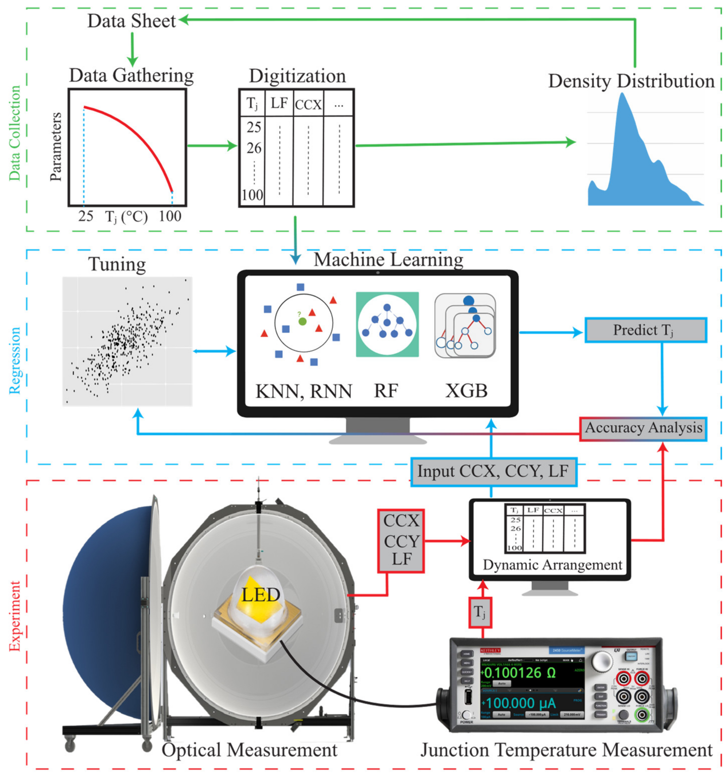
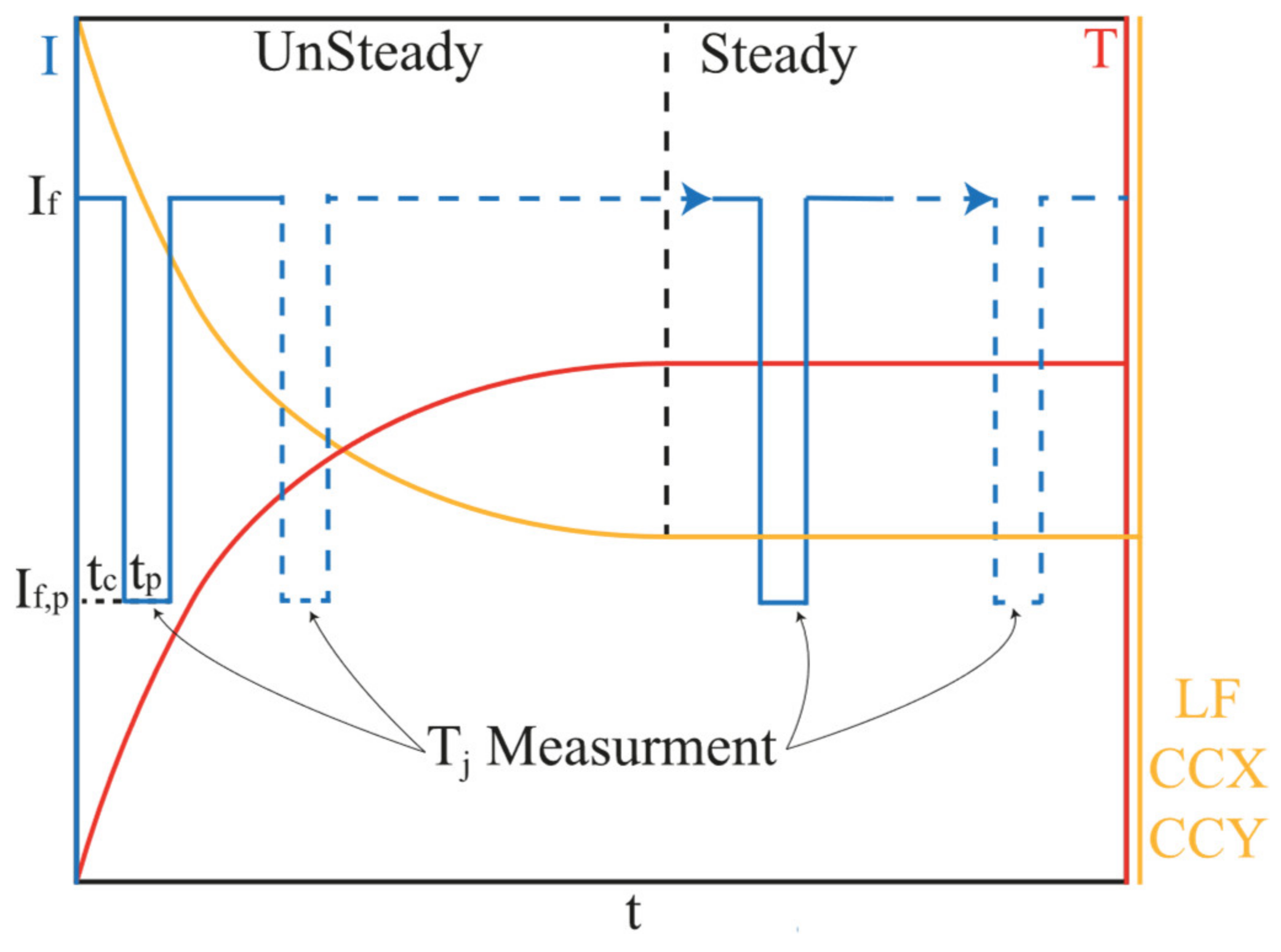
2. Method
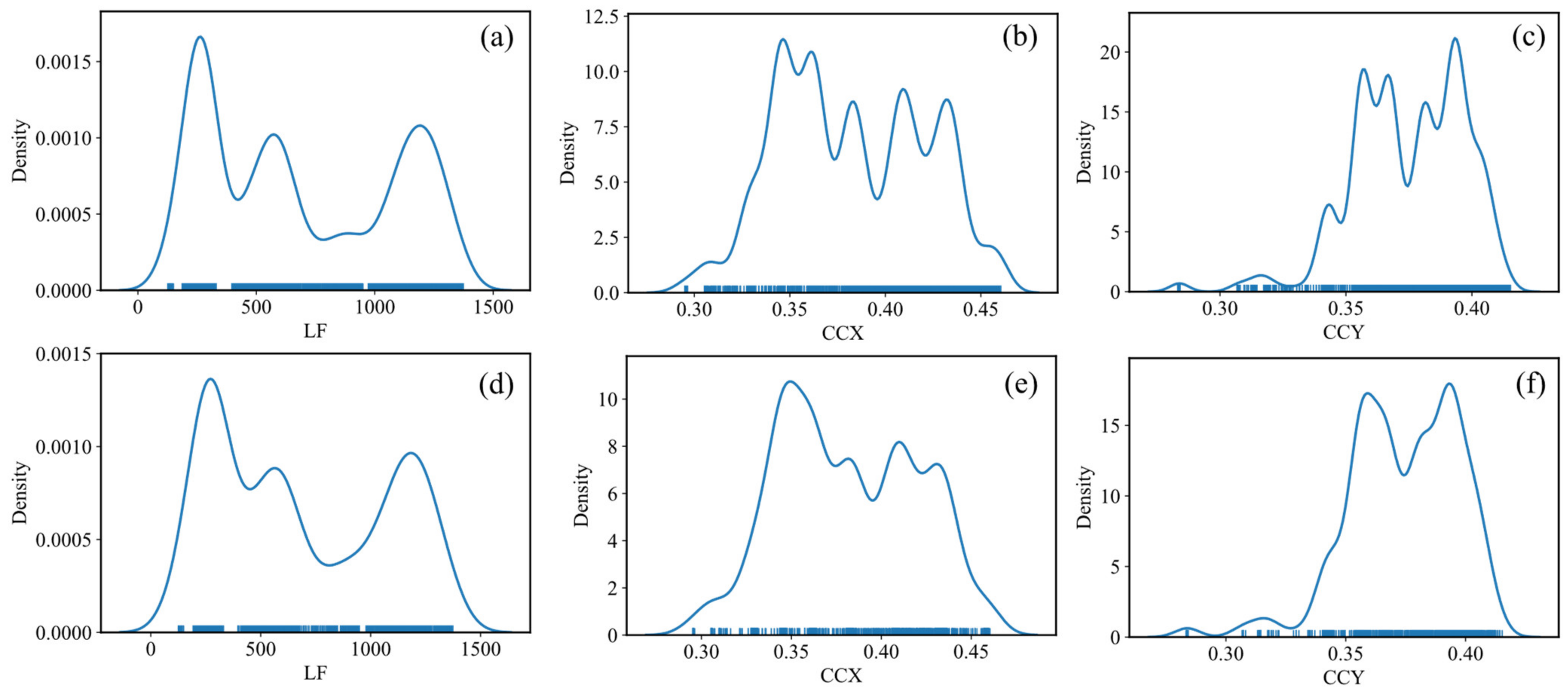
3. Results
4. Conclusions
Author Contributions
Funding
Acknowledgments
Conflicts of Interest
References
- Akasaki, I. Key inventions in the history of nitride-based blue LED and LD. J. Cryst. Growth 2007, 300, 2–10. [Google Scholar] [CrossRef]
- Elliott, C. Energy Savings Forecast of Solid-State Lighting in General Illumination Applications; Navigant Consulting, DOE/EERE 2001; Other: 8172 United States 10.2172/1607661 Other: 8172 EE-LIBRARY English. 2019. Available online: https://www.osti.gov/servlets/purl/1607661 (accessed on 2 January 2022).
- Pattison, P.M.; Pattison, L.; Hansen, M.; Tsao, J.; Bardsley, J.N.; Yamada, M.; Taylor, V.; Stober, K. 2016 DOE SSL R&D Plan. In Proceedings of the 2016 DOE SSL R&D Workshop, Raleigh, NC, USA, 2–4 February 2016. [Google Scholar]
- Arik, M.; Becker, C.A.; Weaver, S.E.; Petroski, J. Thermal management of LEDs: Package to system. In Third International Conference on Solid State Lighting; International Society for Optics and Photonics: San Diego, CA, USA, 2004; Volume 5187, pp. 64–75. [Google Scholar]
- Hwang, W.J.; Lee, T.H.; Choi, J.H.; Kim, H.K.; Nam, O.H.; Park, Y.J.; Shin, M.W. Thermal investigation of GaN-based laser diode package. IEEE Trans. Compon. Packag. Technol. 2007, 30, 637–642. [Google Scholar] [CrossRef]
- Mroziewicz, B.; Bugajski, M.; Nakwaski, W. Physics of Semiconductor Lasers; Elsevier: Amsterdam, The Netherlands, 1991; pp. 400–423. [Google Scholar]
- Azarifar, M.; Cengiz, C.; Arik, M. Particle based investigation of self-heating effect of phosphor particles in phosphor converted light emitting diodes. J. Lumin. 2021, 231, 117782. [Google Scholar] [CrossRef]
- Azarifar, M.; Doğacan, K.; Dönmezer, N. Thermal spreading performance of gan-on-diamond substrate hemts with localized joule heating. Isı Bilimi Tekniği Dergisi 2019, 39, 111–119. [Google Scholar]
- Muzychka, Y.S.; Yovanovich, M.; Culham, J. Thermal spreading resistance in compound and orthotropic systems. J. Thermophys. Heat Transf. 2004, 18, 45–51. [Google Scholar] [CrossRef] [Green Version]
- Yovanovich, M.M.; Muzychka, Y.S.; Culham, J.R. Spreading resistance of isoflux rectangles and strips on compound flux channels. J. Thermophys. Heat Transf. 1999, 13, 495–500. [Google Scholar] [CrossRef]
- Azarifar, M.; Donmezer, N. A multiscale analytical correction technique for two-dimensional thermal models of AlGaN/GaN HEMTs. Microelectron. Reliab. 2017, 74, 82–87. [Google Scholar] [CrossRef]
- Titkov, I.E.; Karpov, S.Y.; Yadav, A.; Zerova, V.L.; Zulonas, M.; Galler, B.; Strassburg, M.; Pietzonka, I.; Lugauer, H.-J.; Rafailov, E.U. Temperature-dependent internal quantum efficiency of blue high-brightness light-emitting diodes. IEEE J. Quantum Electron. 2014, 50, 911–920. [Google Scholar] [CrossRef] [Green Version]
- Meneghini, M.; De Santi, C.; Tibaldi, A.; Vallone, M.; Bertazzi, F.; Meneghesso, G.; Zanoni, E.; Goano, M. Thermal droop in III-nitride based light-emitting diodes: Physical origin and perspectives. J. Appl. Phys. 2020, 127, 211102. [Google Scholar] [CrossRef]
- Sotoodeh, M.; Khalid, A.H.; Rezazadeh, A.A. Empirical low-field mobility model for III–V compounds applicable in device simulation codes. J. Appl. Phys. 2000, 87, 2890–2900. [Google Scholar] [CrossRef]
- Ashdown, I.; Salsbury, M. Peak wavelength shifts and opponent color theory. In Seventh International Conference on Solid State Lighting; International Society for Optics and Photonics: San Diego, CA, USA, 2007; Volume 6669, p. 66690C. [Google Scholar]
- Chhajed, S.; Xi, Y.; Gessmann, T.; Xi, J.-Q.; Shah, J.M.; Kim, J.K.; Schubert, E.F. Junction temperature in light-emitting diodes assessed by different methods. In Light-Emitting Diodes: Research, Manufacturing, and Applications IX; International Society for Optics and Photonics: San Jose, CA, USA, 2005; Volume 5739, pp. 16–24. [Google Scholar]
- Arik, M.; Kulkarni, K.S.; Royce, C.; Weaver, S. Developing a standard measurement and calculation procedure for high brightness LED junction temperature. In Proceedings of the Fourteenth Intersociety Conference on Thermal and Thermomechanical Phenomena in Electronic Systems (ITherm), Orlando, FL, USA, 14–18 March 2014; pp. 170–177. [Google Scholar]
- Xi, Y.; Gessmann, T.; Xi, J.; Kim, J.K.; Shah, J.M.; Schubert, E.F.; Fischer, A.J.; Crawford, M.H.; Bogart, K.H.A.; Allerman, A.A. Junction temperature in ultraviolet light-emitting diodes. Jpn. J. Appl. Phys. 2005, 44, 7260. [Google Scholar] [CrossRef] [Green Version]
- Chhajed, S.; Xi, Y.; Li, Y.-L.; Gessmann, T.; Schubert, E. Influence of junction temperature on chromaticity and color-rendering properties of trichromatic white-light sources based on light-emitting diodes. J. Appl. Phys. 2005, 97, 054506. [Google Scholar] [CrossRef]
- Chen, K.; Narendran, N. Estimating the average junction temperature of AlGaInP LED arrays by spectral analysis. Microelectron. Reliab. 2013, 53, 701–705. [Google Scholar] [CrossRef]
- Tamura, T.; Setomoto, T.; Taguchi, T. Illumination characteristics of lighting array using 10 candela-class white LEDs under AC 100 V operation. J. Lumin. 2000, 87, 1180–1182. [Google Scholar] [CrossRef]
- Chen, H.-T.; Tan, S.-C.; Hui, S. Color variation reduction of GaN-based white light-emitting diodes via peak-wavelength stabilization. IEEE Trans. Power Electron. 2013, 29, 3709–3719. [Google Scholar] [CrossRef] [Green Version]
- Gu, Y.; Narendran, N. A noncontact method for determining junction temperature of phosphor-converted white LEDs. In Third International Conference on Solid State Lighting; International Society for Optics and Photonics: San Diego, CA, USA, 2004; Volume 5187, pp. 107–114. [Google Scholar]
- Yang, T.-H.; Huang, H.-Y.; Sun, C.-C.; Glorieux, B.; Lee, X.-H.; Yu, Y.-W.; Chung, T.-Y. Noncontact and instant detection of phosphor temperature in phosphor-converted white LEDs. Sci. Rep. 2018, 8, 296. [Google Scholar] [CrossRef] [PubMed]
- Lin, Y.; Gao, Y.-L.; Lu, Y.-J.; Zhu, L.-H.; Zhang, Y.; Chen, Z. Study of temperature sensitive optical parameters and junction temperature determination of light-emitting diodes. Appl. Phys. Lett. 2012, 100, 202108. [Google Scholar] [CrossRef] [Green Version]
- Wang, T.; Nakagawa, D.; Wang, J.; Sugahara, T.; Sakai, S. Photoluminescence investigation of InGaN/GaN single quantum well and multiple quantum wells. Appl. Phys. Lett. 1998, 73, 3571–3573. [Google Scholar] [CrossRef]
- Wang, Y.; Pan, M.; Li, T. Comprehensive study of internal quantum efficiency of high-brightness GaN-based light-emitting diodes by temperature-dependent electroluminescence method. In Light-Emitting Diodes: Materials, Devices, and Applications for Solid State Lighting XVIII; International Society for Optics and Photonics: San Francisco, CA, USA, 2014; Volume 9003, p. 90030D. [Google Scholar]
- Hao, R.; Chen, L.; Wu, J.; Fan, D.; Wu, Y.; Liang, S. Effects of growth temperature change in quantum well on luminescence performance and optical spectrum. Optik 2021, 235, 166606. [Google Scholar] [CrossRef]
- Li, J.; Chen, D.; Li, K.; Wang, Q.; Shi, M.; Cheng, C.; Leng, J. Carrier Dynamics in InGaN/GaN-based green LED under different excitation sources. Crystals 2021, 11, 1061. [Google Scholar] [CrossRef]
- Takeuchi, T.; Sota, S.; Katsuragawa, M.; Komori, M.; Takeuchi, H.; Amano, H.; Akasaki, I. Quantum-confined Stark effect due to piezoelectric fields in GaInN strained quantum wells. Jpn. J. Appl. Phys. 1997, 36, L382. [Google Scholar] [CrossRef]
- Mukai, T.; Yamada, M.; Nakamura, S. Characteristics of InGaN-based UV/blue/green/amber/red light-emitting diodes. Jpn. J. Appl. Phys. 1999, 38, 3976. [Google Scholar] [CrossRef]
- Krames, M.R.; Christenson, G.; Collins, D.; Cook, L.W.; Craford, M.G.; Edwards, A.; Fletcher, R.M.; Gardner, N.F.; Goetz, W.K.; Imler, W.R.; et al. High-brightness AlGaInN light-emitting diodes. In Light-Emitting Diodes: Research, Manufacturing, and Applications IV; International Society for Optics and Photonics: San Jose, CA, USA, 2000; Volume 3938, pp. 2–12. [Google Scholar]
- Smith, T.; Guild, J. The CIE colorimetric standards and their use. Trans. Opt. Soc. 1931, 33, 73. [Google Scholar] [CrossRef]
- Stockman, A.; Sharpe, L.T. The spectral sensitivities of the middle-and long-wavelength-sensitive cones derived from measurements in observers of known genotype. Vis. Res. 2000, 40, 1711–1737. [Google Scholar] [CrossRef] [Green Version]
- David, A.; Young, N.G.; Lund, C.; Craven, M.D. The physics of recombinations in III-nitride emitters. ECS J. Solid State Sci. Technol. 2019, 9, 016021. [Google Scholar] [CrossRef]
- Liu, S.; Luo, X. LED Packaging for Lighting Applications: Design, Manufacturing, and Testing; John Wiley & Sons: New York, NY, USA, 2011. [Google Scholar]
- Yuan, C.C.; Fan, J.; Fan, X. Deep machine learning of the spectral power distribution of the LED system with multiple degradation mechanisms. J. Mech. 2021, 37, 172–183. [Google Scholar] [CrossRef]
- Ibrahim, M.S.; Fan, J.; Yung, W.K.C.; Prisacaru, A.; van Driel, W.; Fan, X.; Zhang, G. Machine Learning and Digital Twin Driven Diagnostics and Prognostics of Light-Emitting Diodes. Laser Photonics Rev. 2020, 14, 2000254. [Google Scholar] [CrossRef]
- Lu, K.; Zhang, W.; Sun, B. Multidimensional data-driven life prediction method for white LEDs based on BP-NN and improved-adaboost algorithm. IEEE Access 2017, 5, 21660–21668. [Google Scholar] [CrossRef]
- Liu, H.; Guo, K.; Zhang, Z.; Yu, D.; Zhang, J.; Ning, P.; Cheng, J.; Li, X.; Niu, P. High-power LED photoelectrothermal analysis based on backpropagation artificial neural networks. IEEE Trans. Electron Devices 2017, 64, 2867–2873. [Google Scholar] [CrossRef]
- Liu, H.; Yu, D.; Niu, P.; Zhang, Z.; Guo, K.; Wang, D.; Zhang, J.; Ma, X.; Jia, C.; Wu, C. Lifetime prediction of a multi-chip high-power LED light source based on artificial neural networks. Results Phys. 2019, 12, 361–367. [Google Scholar] [CrossRef]
- Chang, M.-H.; Chen, C.; Das, D.; Pecht, M. Anomaly detection of light-emitting diodes using the similarity-based metric test. IEEE Trans. Ind. Inform. 2014, 10, 1852–1863. [Google Scholar] [CrossRef]
- Fan, J.; Li, Y.; Fryc, I.; Qian, C.; Fan, X.; Zhang, G. Machine-learning assisted prediction of spectral power distribution for full-spectrum white light-emitting diode. IEEE Photonics J. 2019, 12, 8200218. [Google Scholar] [CrossRef]
- Merenda, M.; Porcaro, C.; Della Corte, F.G. LED junction temperature prediction using machine learning techniques. In Proceedings of the 2020 IEEE 20th Mediterranean Electrotechnical Conference (MELECON), Palermo, Italy, 16–18 June 2020; pp. 207–211. [Google Scholar]
- Azarifar, M.; Cengiz, C.; Arik, M. Dynamic opto-electro-thermal characterization of solid state lighting devices: Measuring the power conversion efficiency at high current densities. J. Phys. D Appl. Phys. 2022, 55, 39. [Google Scholar] [CrossRef]
- Cengiz, C.; Azarifar, M.; Arik, M. Thermal and Optical Characterization of White and Blue Multi-Chip LED Light Engines. In Proceedings of the 2021 20th IEEE Intersociety Conference on Thermal and Thermomechanical Phenomena in Electronic Systems (iTherm), San Diego, CA, USA, 1–4 June 2021; pp. 285–293. [Google Scholar]
- Azarifar, M.; Cengiz, C.; Arik, M. Thermal and optical performance characterization of bare and phosphor converted LEDs through package level immersion cooling. Int. J. Heat Mass Transf. 2022, 189, 122607. [Google Scholar] [CrossRef]
- Kotsiantis, S.B.; Zaharakis, I. Pintelas, P. Supervised machine learning: A review of classification techniques. Emerg. Artif. Intell. Appl. Comput. Eng. 2007, 160, 3–24. [Google Scholar]
- Harrington, P. Machine Learning in Action; Simon and Schuster: New York, NY, USA, 2012. [Google Scholar]
- Altman, N.S. An introduction to kernel and nearest-neighbor nonparametric regression. Am. Stat. 1992, 46, 175–185. [Google Scholar]
- Svetnik, V.; Liaw, A.; Tong, C.; Culberson, J.C.; Sheridan, R.P.; Feuston, B.P. Random forest: A classification and regression tool for compound classification and QSAR modeling. J. Chem. Inf. Comput. Sci. 2003, 43, 1947–1958. [Google Scholar] [CrossRef]
- Chen, T.; He, T.; Benesty, M.; Khotilovich, V.; Tang, Y.; Cho, H.; Chen, K. Xgboost: Extreme gradient boosting. R Package Version 0.4-2 2015, 1, 1–4. [Google Scholar]
- Bachmann, V.; Ronda, C.; Meijerink, A. Temperature quenching of yellow Ce3+ luminescence in YAG: Ce. Chem. Mater. 2009, 21, 2077–2084. [Google Scholar] [CrossRef]


Publisher’s Note: MDPI stays neutral with regard to jurisdictional claims in published maps and institutional affiliations. |
© 2022 by the authors. Licensee MDPI, Basel, Switzerland. This article is an open access article distributed under the terms and conditions of the Creative Commons Attribution (CC BY) license (https://creativecommons.org/licenses/by/4.0/).
Share and Cite
Azarifar, M.; Ocaksonmez, K.; Cengiz, C.; Aydoğan, R.; Arik, M. Machine Learning to Predict Junction Temperature Based on Optical Characteristics in Solid-State Lighting Devices: A Test on WLEDs. Micromachines 2022, 13, 1245. https://doi.org/10.3390/mi13081245
Azarifar M, Ocaksonmez K, Cengiz C, Aydoğan R, Arik M. Machine Learning to Predict Junction Temperature Based on Optical Characteristics in Solid-State Lighting Devices: A Test on WLEDs. Micromachines. 2022; 13(8):1245. https://doi.org/10.3390/mi13081245
Chicago/Turabian StyleAzarifar, Mohammad, Kerem Ocaksonmez, Ceren Cengiz, Reyhan Aydoğan, and Mehmet Arik. 2022. "Machine Learning to Predict Junction Temperature Based on Optical Characteristics in Solid-State Lighting Devices: A Test on WLEDs" Micromachines 13, no. 8: 1245. https://doi.org/10.3390/mi13081245