1. Introduction
The physical phenomenon of quantum mechanical tunneling between source and drain (S/D tunneling) arises when the scaling process of electronic devices enters the regime of channel lengths around and below 10 nm [
1,
2]. Monte Carlo simulations aiming to account for the description of this type of structures (when this tunneling contribution requires attention in the subthreshold regime) were traditionally providing current levels above those obtained from simulators with full quantum transport treatment [
3]. In spite of this drawback, the design and conception of a Multisubband Ensemble Monte Carlo (MS-EMC) tool still provides a very efficient computation technique based on a modular implementation of the specific quantum transport mechanisms involved in the assessment of each device of interest [
4,
5]. For that reason, the improvement of the MS-EMC tool in order to achieve a satisfactory description of the S/D tunneling phenomena is particularly valuable in the context of the present sizes of ultrascaled devices.
To do so, one of the proposed solutions turned out to be the reformulation of the tunneling probability across the potential barrier between source and drain [
6]. This was implemented by means of a non-local approach following the formalism developed in [
7], that introduces an additional term correcting the traditional WKB tunneling probability for 2D simulations. Labeling
x as the transport direction and
z the perpendicular direction affected by confinement, the modified tunneling probability reads as [
8]
where
is the mesh spacing in the periodic direction normal to both transport and confinement dimensions;
a and
b are the limits of the tunneling path;
is the tunneling effective mass of the electron;
is the total energy of the superparticle in the transport plane considering only the projection of the kinetic energy in the direction facing the barrier, and
stands for the energy profile of the
i-th subband.
represents the conventional tunneling probability given by the WKB approximation and reads as
In light of the expression for , its behavior needs to be assessed (due to the term with the negative power) in order to determine for which types of potential barriers it can be used as an appropriate tunneling probability. Should this analysis not be carried out, one might risk to derive untrustworthy conclusions about the S/D importance in those devices where it plays a non-negligible role.
Notice that, in an alternative way to the stochastic conception implied bythe Monte Carlo method, the problem of the lack of validity of the WKB approximation at the turning points of the potential barrier could also be envisaged from a different theoretical perspective employing a wave function formalism. Should this approach be followed, the wave functions would need to be described in in the neighborhoods of the turning points by asymptotic formulas whose leading term would be expressed in terms of Bessel functions.
This paper analyzes the mathematical behavior of the proposed
tunneling probability in the context of the utilizaton of a MS-EMC simulator and delimits the type of potentials for which it proves to be suitable. In
Section 2, we expose the behavior of
for a very simple triangular potential profile, illustrating the nature of the problems to be faced. In
Section 3, we focus on realistic smooth potentials like those provided by solving the Poisson equation and derive the conditions to be fulfilled by them in order to guarantee an adequate utilization of
when simulating with the MS-EMC tool. Finally, the main conclusions are drawn in
Section 4.
2. Reformulated Tunneling Probability Applied to a Simple Potential Barrier
When the carrier impinges on the energy barrier with a certain energy , it is obvious that equals at the point where the carrier enters the barrier (i.e., the point with in the integrals above). The problem arises as long as this leads to a divergence in the integrand of the term with power in (which is something not to be concerned about if one simply handles with tunneling probabilities described by ).
In what follows, and for the ease of treatment, all auxiliary constants will be set to one and
will be written as
with
and
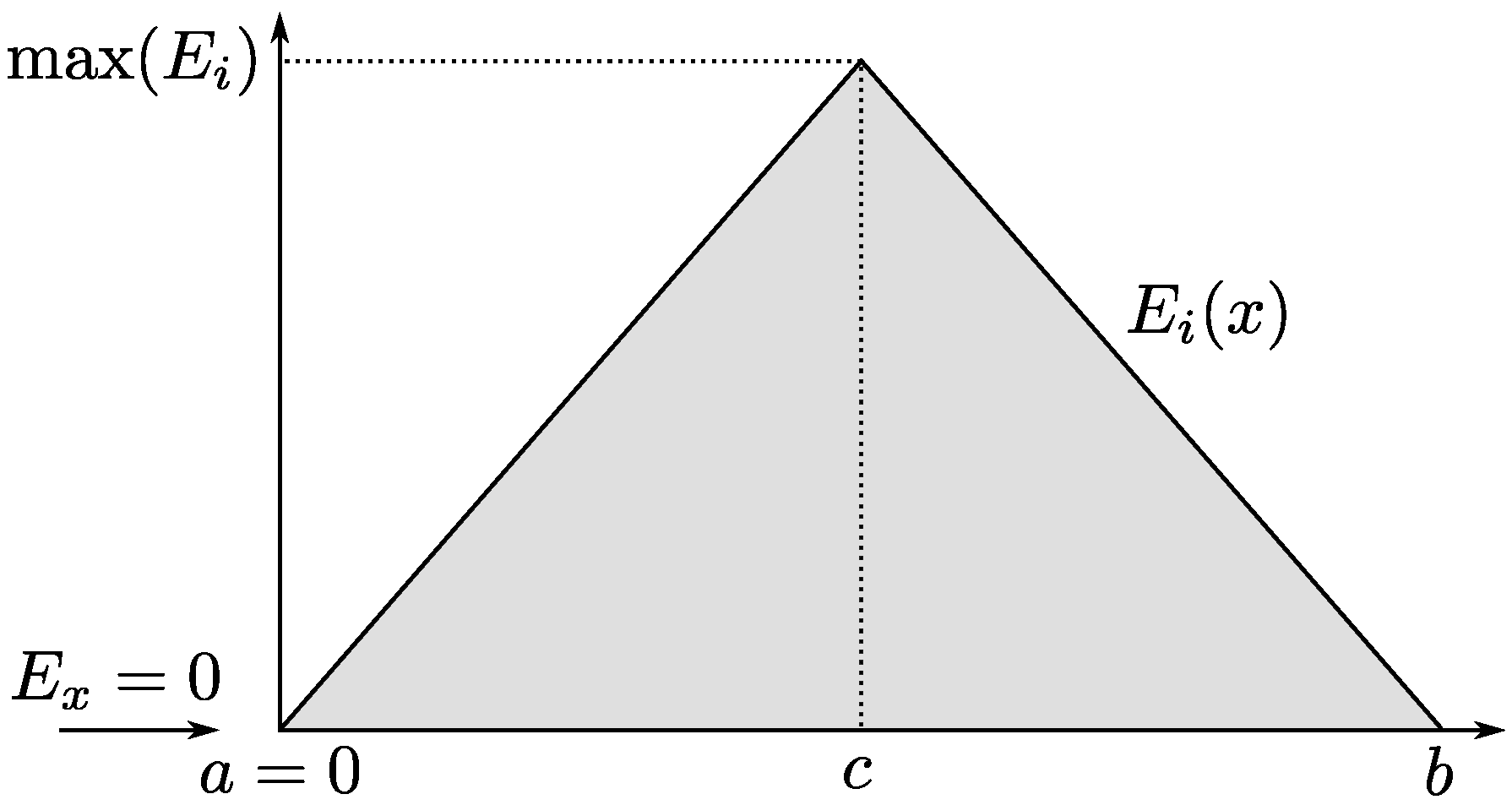
Let us now consider the elementary triangular barrier depicted in
Figure 1 given by
We will suppose that the barrier starts at (i.e., ) and that the carrier hits the barrier with .
In that case,
would read as
where the divergence disappears thanks to the integral. However, for this simple example, the resulting behavior of
is incompatible with that corresponding to a well behaved tunneling probability, namely:
Therefore, careful assessment needs to be carried out as to determine for which type of potential barriers the utilization of might be suitable.
3. Reformulated Tunneling Probability Applied to Smooth Potential Barriers
Let us now consider the situation where the potential barrier can be described by a smooth differentiable function between the limits of integration. This situation differs from the simplified scenario analyzed in the previous section (as far as the triangular barrier was not smooth at its maximum), but proves to be more realistic taking into account the usual shape of the potential barriers to be found in scenarios where source to drain tunneling arises.
3.1. Boundedness
According to the form of
, and in order to keep its integral finite when evaluating it at
for a given
, we need that
If we compute this limit for an energy barrier
, we see that both numerator and denominator tend to zero as
x approaches
. For that reason, the limit can be computed by l’Hôpital as
that equals zero provided that the barrier has a certain slope at the impinging point
, which is inherent to the nature of the barrier itself. The reasoning is exactly analogous for the exit point
. Observe that this result is independent of the shape of
, the only requirement is that
at
and
.
Up to this point, the only thing that is guaranteed is that
will remain finite for
provided that
at
and
. However, we still need
not to go to zero or to infinity as
tends to
. As we are supposing
to be smooth, it can be expanded in Taylor series around the point
where
attains its maximum. This leads to
with
,
and
. Now suppose that, for simplicity, the potential is centered at the origin so that
. The above expression reduces to
Since we are interested in the behavior when tends to , this is the same as saying that we are interested in the behavior of the Taylor series when x tends to zero or, in other words, that the key of the analysis relies on the order of the first non vanishing coeficient of the expansion, which is the one controlling how approaches to its maximum.
Let us suppose that
(which leads to
because the potential has a maximum). In that case, we can neglect all the terms of higher order and obtain a simple inverted parabolic potential. If we compute the value of
, we obtain
This expression is independent of and remains constant when tends to , thus providing a finite non zero value of even at the top of the barrier.
On the other hand, if
(which means that the barrier will feature a certain plateau at its top), the next non vanishing (and negative) coeficient will necessarily be
with
j even, and again all orders above it can be neglected if we want to analyze the behavior when
tends to
. The corresponding expression for
is then
with
The computation of
by means of elliptic integrals leads to
where
stands for the gamma function. The presence of the term
in the denominator makes
diverge as
approaches
. This result indicates that the potential barrier must necessarily possess a cuadratic behavior close to its maximum, and that the appearance of an upper plateau (for example, if the gate length is not too aggressively scaled) deprives
from its physical meaning. Fortunately, given that S/D tunneling becomes relevant for narrow potentials, this requirement will very likely be satisfied in most of the cases of interest.
3.2. Monotonicity
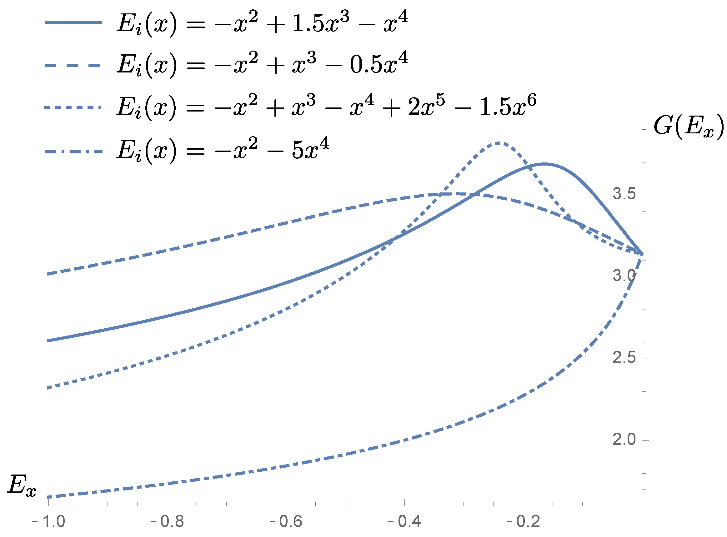
The fact of assuring that remains bounded and non zero for any of the impinging energies of interest is not enough for guaranteeing an appropriate behavior of . We need to demand monotonicity too. In other words, the tunneling probability needs to increase as approaches .
Note that, in principle, and from the form of
in Equation (
3), one cannot affirm that this will always be the case since
results from the product of a function of
and a function of
, and
can very well not be monotonic as shown in
Figure 2 for different barrier examples fulfilling boundedness. It is therefore desirable to derive a condition that ensures the monotonicity of
once the shape of the potential is known.
For that aim, we shall demand that
. In our case, and considering that
always evaluates to a positive number, we can use that
which proves to be a more convenient condition for studying the behavior of
recalling its expression as a function of
and
. Therefore, using Equation (
3) we obtain that
For calculating the derivatives of
and
we need to apply the Leibniz rule, which leads to
Taking the relationship between
and
of Equation (
5), we observe that
Now, since
evaluates to zero when
and
, the last equation is simply
If we apply this result to Equation (
19) and use that
is always positive, we obtain that
This last inequality constitutes a simple way of formulating the condition that must be satisfied once the shape of the potential barrier
is known in order to guarantee the monotonicity of
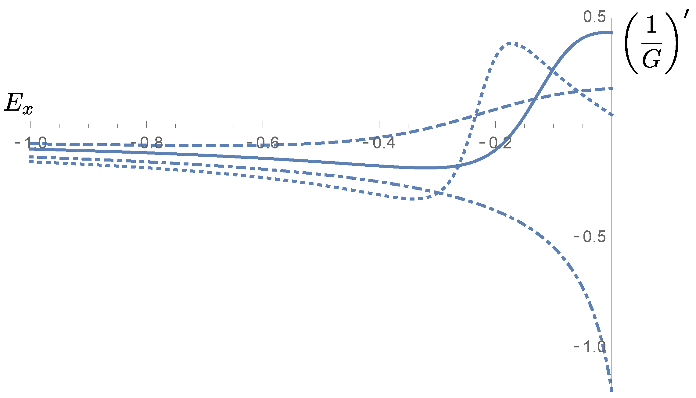
. In
Figure 3, we observe that three of the example barriers of
Figure 2 fulfill this condition, so that the probability
would be well behaved for them. On the other hand, for the dashed dotted curve, the probability
would not be monotonic.
We conclude that boundedness does not necessarily imply monotonicity for . For a given potential, both requirements would need to be verified separately.
4. Conclusions
One of the envisageable solutions to improve the accuracy of the S/D tunneling current computation in a MS-EMC simulator is to redefine the tunneling probability by which it is estimated. However, in light of the resulting expression obtained from a non-local reformulation, its applicability is not automatically well defined for any potential barrier that might arise between source and drain regions. We have demonstrated that boundedness of the tunneling probability is ensured for potentials not featuring a flat region around its maximum (i.e., those with non-vanishing quadratic terms when expanded in series). With respect to monotonicity, this property is not automatically ensued from the boundedness of the tunneling probability and requires, in turn, a certain constraint on the boundedness of the derivative of the prefactor modifying the WKB tunneling probability.
Author Contributions
Conceptualization, J.L.P. and C.M.-B.; methodology, J.L.P. and A.P.; validation, C.M.-B. and L.D.; formal analysis, J.L.P. and A.P.; investigation, J.L.P. and C.M.-B.; writing—original draft preparation, J.L.P.; writing—review and editing, L.D., A.P. and C.S.; visualization, C.M.-B.; supervision, F.G.; project administration, J.L.P.; funding acquisition, C.N. and L.D. All authors have read and agreed to the published version of the manuscript.
Funding
This research was funded by Junta de Andalucia, grant number P18-RT-4826.
Institutional Review Board Statement
Not applicable.
Informed Consent Statement
Not applicable.
Data Availability Statement
Not applicable.
Conflicts of Interest
The authors declare no conflict of interest. The funders had no role in the design of the study; in the collection, analyses, or interpretation of data; in the writing of the manuscript, or in the decision to publish the results.
Abbreviations
The following abbreviations are used in this manuscript:
| S/D | Source to drain |
| MS-EMC | Multisubband Ensemble Monte Carlo |
| WKB | Wentzel-Kramers-Brillouin |
References
- Iwai, H. Future of nano CMOS technology. Solid-State Electron. 2015, 112, 56–67. [Google Scholar] [CrossRef]
- Grillet, C.; Logoteta, D.; Cresti, A.; Pala, M.G. Assessment of the Electrical Performance of Short Channel InAs and Strained Si Nanowire FETs. IEEE Trans. Electron. Devices 2017, 64, 2425–2431. [Google Scholar] [CrossRef]
- Medina-Bailon, C.; Sampedro, C.; Padilla, J.L.; Godoy, A.; Donetti, L.; Gamiz, F.; Asenov, A. MS-EMC vs. NEGF: A comparative study accounting for transport quantum corrections. In Proceedings of the Joint International EUROSOI Workshop and International Conference on Ultimate Integration on Silicon (EUROSOI-ULIS 2018), Granada, Spain, 19–21 March 2018; pp. 1–4. [Google Scholar]
- Sampedro, C.; Medina-Bailon, C.; Donetti, L.; Padilla, J.L.; Navarro, C.; Marquez, C.; Gamiz, F. Multi-Subband Ensemble Monte Carlo Simulator for Nanodevices in the End of the Roadmap. In Large-Scale Scientific Computing, Proceedings of the 12th International Conference, LSSC 2019, Sozopol, Bulgaria, 10–14 June 2019; Lecture Notes in Computer Science; Lirkov, I., Margenov, S., Eds.; Springer: New York, NY, USA, 2019; Volume 11958, pp. 438–445. [Google Scholar]
- Medina-Bailon, C.; Padilla, J.L.; Sadi, T.; Sampedro, C.; Godoy, A.; Donetti, L.; Georgiev, V.; Gamiz, F.; Asenov, A. Multisubband Ensemble Monte Carlo Analysis of Tunneling Leakage Mechanisms in Ultrascaled FDSOI, DGSOI and FinFET Devices. IEEE Trans. Electron. Devices 2019, 66, 1145–1152. [Google Scholar] [CrossRef]
- Medina-Bailon, C.; Carrillo-Nunez, H.; Lee, J.; Sampedro, C.; Padilla, J.L.; Donetti, L.; Georgiev, V.; Gamiz, F.; Asenov, A. Quantum Enhancement of a S/D Tunneling Model in a 2D MS-EMC Nanodevice Simulator: NEGF Comparison and Impact of Effective Mass Variation. Micromachines 2020, 11, 204. [Google Scholar] [CrossRef] [PubMed] [Green Version]
- Nunez, H.C.; Ziegler, A.; Luisier, M.; Schenk, A. Modeling direct band-to-band tunneling: From bulk to quantum-confined semiconductor devices. J. Appl. Phys. 2015, 117, 243501. [Google Scholar]
- Medina-Bailon, C.; Padilla, J.L.; Sampedro, C.; Donetti, L.; Georgiev, V.; Gamiz, F.; Asenov, A. Self-Consistent Enhanced S/D Tunneling Implementation in a 2D MS-EMC Nanodevice Simulator. Micromachines 2021, 12, 601. [Google Scholar] [CrossRef] [PubMed]
| Publisher’s Note: MDPI stays neutral with regard to jurisdictional claims in published maps and institutional affiliations. |
© 2022 by the authors. Licensee MDPI, Basel, Switzerland. This article is an open access article distributed under the terms and conditions of the Creative Commons Attribution (CC BY) license (https://creativecommons.org/licenses/by/4.0/).


 ,
, 


