Review

Power Losses Models for Magnetic Cores: A Review

by
Daniela Rodriguez-Sotelo
1,†,
Martin A. Rodriguez-Licea
2,†,
Ismael Araujo-Vargas
3,
Juan Prado-Olivarez
1,
Alejandro-Israel Barranco-Gutiérrez
1 and
Francisco J. Perez-Pinal
1,*,†
1
Tecnológico Nacional de México, Instituto Tecnológico de Celaya, Antonio García Cubas Pte. 600, Celaya 38010, Mexico
2
CONACYT, Tecnológico Nacional de México, Instituto Tecnológico de Celaya, Antonio García Cubas Pte. 600, Celaya 38010, Mexico
3
Escuela Superior de Ingeniería Mecánica y Eléctrica (ESIME), Unidad Culhuacán, Instituto Politécnico Nacional, Mexico City 04260, Mexico
*
Author to whom correspondence should be addressed.
These authors contributed equally to this work.
Micromachines 2022, 13(3), 418; https://doi.org/10.3390/mi13030418
Submission received: 3 February 2022 / Revised: 24 February 2022 / Accepted: 25 February 2022 / Published: 7 March 2022

Abstract

:
In power electronics, magnetic components are fundamental, and, unfortunately, represent one of the greatest challenges for designers because they are some of the components that lead the opposition to miniaturization and the main source of losses (both electrical and thermal). The use of ferromagnetic materials as substitutes for ferrite, in the core of magnetic components, has been proposed as a solution to this problem, and with them, a new perspective and methodology in the calculation of power losses open the way to new design proposals and challenges to overcome. Achieving a core losses model that combines all the parameters (electric, magnetic, thermal) needed in power electronic applications is a challenge. The main objective of this work is to position the reader in state-of-the-art for core losses models. This last provides, in one source, tools and techniques to develop magnetic solutions towards miniaturization applications. Details about new proposals, materials used, design steps, software tools, and miniaturization examples are provided.

1. Introduction

It is a fact that magnetic components are an essential part of our lives. We can find them in almost anything of quotidian use, from simple things such as cell phone charges [1] to TVs and home appliances. However, they have become more relevant in the development of electric and hybrid vehicles, electric machines [2], renewable energy systems [3,4,5,6], and recently in implanted electronics [7,8] to open the possibility to micro-scale neural interfaces [9]. Inside these devices and systems, a power stage is conformed by magnetic and electronic components.
A few years ago, these power stages used to be bigger and heavier, and they had considerable energy losses making them less efficient. Nowadays, silicon carbide (SiC) and gallium nitride (GaN) switching devices have improved power electronics, making them smaller and faster [10,11]. Notwithstanding, magnetic components oppose miniaturization; these remain stubbornly large and lossy [12]. In a modern power converter, magnetics are approximately half of the volume and weight, and they are the main source of power losses [13,14].
The trend in power electronics has two explicit purposes for the design of magnetic components. The former is to make maximum use of magnetics capabilities, achieving multiple functions from a single component [12]. The latter consists of minimizing the size of magnetic components substituting ferrite (the leading material in their fabrication) with ferromagnetic materials [15]. Those materials have a higher saturation point than ferrite, high permeability and are based on iron (Fe) and metallic elements (Si, Ni, Cr, and Co). Some examples of these kinds of material are Fe-Si alloys, powder cores, amorphous materials, and nanocrystal material [16,17,18].
The design of magnetic components is the key to achieving two purposes. The design parameters are intimately dependent on geometric structure, excitation conditions, and magnetic properties such as power losses that determine if a core magnetic is suitable to be part of a magnetic component [19]. Power losses in magnetic components are important design parameters; which limit many high-frequency designs.
Power losses in a magnetic component are divided into two core power losses and winding power losses. Core power losses are related to the selection of the material to make the core of inductors and transformers; in this case, parameters such as frequency operating range, geometric shape, volume, weight, temperature operating range, magnetic saturation point, and relative permeability must be considered [20]. On the other hand, winding losses are related to phenomena such as skin effect, direct current (DC) and alternating current(AC) resistance in a conductor, and proximity effect [19,21,22]. Those phenomena increase the volume of a winding structure [23]. One way to overcome this kind of loss is by using Litz wire [24].
Nowadays, there are several models for studying, predicting, and analyzing the power losses in the ferromagnetic cores of magnetic components. However, many of them have been developed to work in a limited frequency range, temperature and low magnetic flux [25]. Usually, the ferromagnetic cores’ manufacturers provide the graphs of the core losses in their datasheets, which it is commonly obtained with sinusoidal signal tests and for specific values of frequency (f) and magnetic flux (B) [26].
There are many ways to calculate the power losses in magnetic materials. The original Steinmetz equation is one of them; however, to the best of the author’s knowledge, it is not always the best option. In the author’s opinion, selecting a method to calculate power core losses must be based on its versatility to vary their measurement’s parameters [27].
This document aims to provide the reader with a general panorama about the core power losses in ferromagnetic materials, emphasising the diverse models found in the literature, announcing their characteristics, advantages, and limitations. Besides, it will present a relationship about magnetic materials and tested models. Any magnetic component designer must know the basic methods, core losses’ models, the conditions at which they are valid, and their mathematical fundamentals. Magnetic and thermal losses, calculus and modelling are open research areas due to the non-linear features of ferromagnetic materials, the complexity of developing a unique power core losses model for the overall ferromagnetic materials, and their respective validations.
The organization of this work consists of the following sections. In Section 2, the reader will find information about the characteristics of each ferromagnetic material. Losses in magnetic components are reviewed in Section 3. In Section 4, general core losses models are mentioned as empirical core losses proposals. Features of Finite Element Method software are given in Section 5. The design process of a magnetic component is discussed in Section 6; on the other hand, the importance of the core losses methods in miniaturization of magnetic devices is summarized in Section 7. The discussion of this work is presented in Section 8, and finally, in Section 9, conclusions are provided.

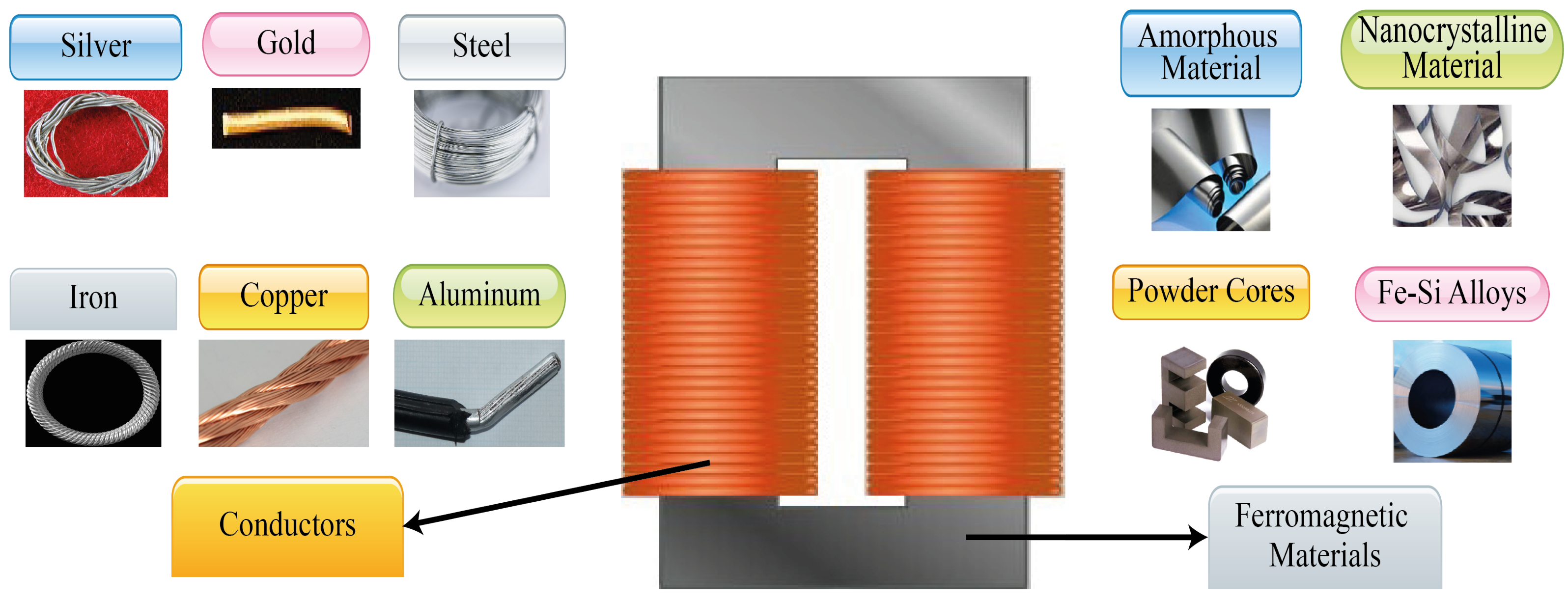
2. Ferromagnetic Alloys

Ferromagnetic materials are exciting materials, where several of their physical properties and chemical micro-structure allow being controlled. Susceptibilities, permeabilities, the shape of the hysteresis loop, power loss, coercivity, remanence, and magnetic induction are some examples of no intrinsic properties [18]. The saturation magnetization and the Curie temperature are the only intrinsic properties [17,18].
The magnetic behavior is ruled by the dipole moments’ interaction of their atoms within an external magnetic field [28]. Ferromagnetic materials have strong magnetic properties due to their magnetic moments that tend to line up easily along an outward magnetic field direction [29]. These materials also have the property of remaining partially magnetized even when the external magnetic field is removed; this means that they can quickly change their magnetic polarization by applying a small field. Ferromagnetic materials are also profitable materials due to being composed by Fe, one of the eight more abundant elements on Earth [30].
Ferromagnetic materials are used in the core of magnetic components; they are classified in Fe-Si alloys, powder cores, amorphous material, and nanocrystalline material; on the other hand, materials as silver, gold, copper, aluminium, iron, steel, among others, are used in windings Figure 1. Except for powder cores, the rest of them are rolled materials [31]; in the following sections, the importance of this fact in the core losses calculation will be detailed. Each one has specific magnetic properties, manufacturing processes, and physical features that determine its feasibility [32].
Fe-Si alloys are alloys based on Fe with small quantities of Si (not more than 4.5%). These alloys are attractive due to their reasonable cost and magnetic properties [44]. There are two kinds: grain non-oriented sheets (GNO) and grain-oriented sheets (GO) [30]. At present, GO material represents 80% of the electrical devices market [17,45].
On the other hand, powder cores are fabricated from metallic powders, typically iron; however, those can be composed of alloys with P, Si and Co [46]. The manufacturing process of this kind of material allows special fabrication geometry cores. Usually, powder cores are mixed with a binder or insulating material to reduce magnetic losses at high frequencies [47]. According to the material used in their fabrication, those can be classified into four groups: iron powder core, molybdenum permalloy powder cores (MPP), high flux powder cores, and sendust cores, also called Kool M μ [48]. These materials present the more recent advances in magnetic elements [49].
Amorphous alloys or metallic glasses are materials without crystalline order [50]. Those alloys are very strong and hard, but also ductile. They contain approximately 80% of particles of Fe, Ni, Co, and their combinations; and 20% of metalloids particles or glass formed elements (C, Al, B, Si, and P) [51,52].
Nanocrystalline alloys consist of a Fe-Si ultra-thin grain alloy with a few quantities of Cu and Nb. Their manufacturing process is very similar to amorphous alloys [53]. Nanocrystals are materials with high mechanical hardness and extremely fragile. The four main kinds are: finemet, nanoperm, hitperm, and nanomet [54,55].
Nanocrystalline, amorphous and Fe-Si alloys are the materials more used in power electronics, so they have been widely studied, especially in terms of core power losses. In rolled materials as Fe-Si alloys and amorphous materials, their magnetic properties depend on the sheet’s thickness (around a few mm, and 5–50 μ m, respectively). Instead, in nanocrystalline alloys, magnetic properties depend on the diameter of their grains (of the order of 10–15 nm). Rolled materials are susceptible to Eddy currents and skin losses. In contrast, powder cores’ magnetic properties can be manipulated during their manufacturing process, which includes the relative permeability variation according to the magnetic field intensity, high saturation point, fringing flux elimination, soft saturation, among others.

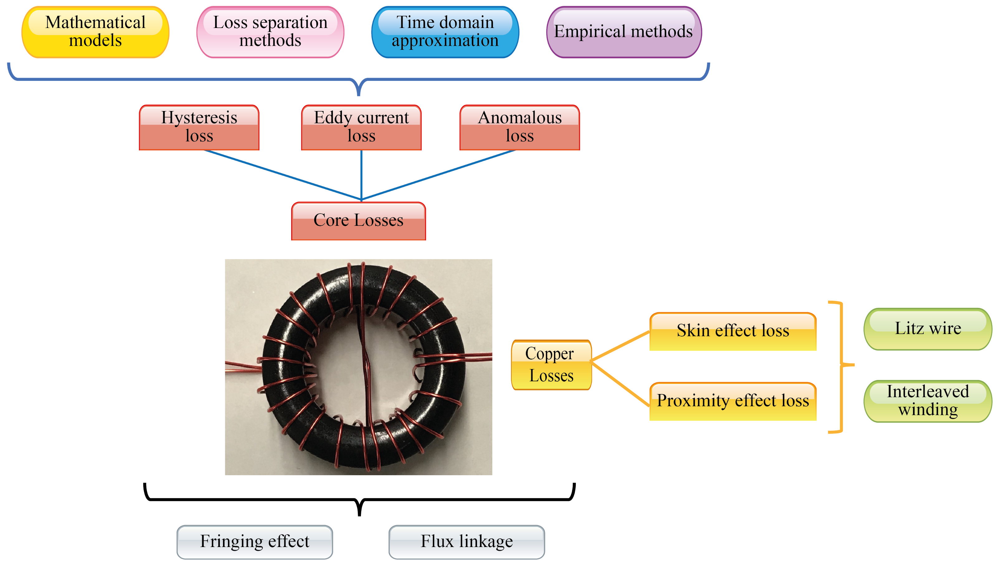
3. Losses in Magnetic Components

To any magnetic component designer, a real challenge to overcome is getting a magnetic component with high efficiency, small size, low cost, convenience, and low losses [56]. Usually, losses are the common factor in all requirements announced before; losses are the most difficult challenges to beat in a magnetic component.
Losses in a magnetic component are divided in two groups: core losses and winding losses (also called copper losses), [57]. Figure 2 shows each one of them, as well as their causing phenomena, methods, models, techniques and elements associated with them; nonetheless, phenomena such as the fringing effect and the flux linkage many times are not considered in the losses model. Still, they are necessary to achieve a complete losses model in any magnetic component.
Current windings generate the flux linkage density; therefore, it is the sum of the flux enclosed of each one of the turns wound around the core, the flux linkage linked them [50,59]. Flux linkage depends on the conductor’s geometry and the quantity of flux contained in it. In the gap between windings is the maximum flux linkage [60,61,62].
Otherwise, the fringing effect is the counterpart of flux linkage; this is, the fringing effect is presented around the air gap instead of the windings of the magnetic component. This phenomenon depends on core geometry and core permeability, to higher permeability the fringing effect is low [50].
The copper losses are caused by the flow of DC and AC through the windings of a magnetic component, where losses always are more significant for AC than DC [63,64]. The circulating current in the windings generates Eddy phenomena as Eddy currents, skin effect loss and, proximity effect loss.
The skin effect and the proximity effect loss are linked to the conductor size, frequency, permeability and distance between winding wires. For the first of them, the current distribution trough the cross-area of the wire will define the current density in it. The skin effect and the proximity effect loss are linked to the winding wires. For the first of them, the current distribution through the cross-area of the wire will define the current density in it. It means that the conductor will have a uniform distribution for DC, higher on its surface and lower in its center for AC distribution [65].
The proximity effect is similar to the skin effect, but in this case, it is generated by the current carried nearby conductors [50,65]. Eddy currents are induced in a wire in this kind of loss due to a variant magnetic field in the vicinity of conductors at high frequency [46,66].
The Litz wire and interleaved windings help minimize winding losses in magnetic components, both are widely used currently. Indeed, interleaved windings are very efficient in high-frequency planar magnetics [67,68].
On the other hand, core losses directly depend on the intrinsic and extrinsic core materials’ characteristics. Core losses are related to hysteresis loop, Eddy currents, and anomalous or residual losses. Without matter, the core losses model chosen by the magnetic component designer will be based on those three primary losses; core loss models will be detailed in the next section. Besides, core losses depend on the core’s geometry and the core intrinsic properties’ such as permeability, flux density, Curie temperature, among others [69,70,71]. Many methods and models have been developed; all of them have the predominant interest in studying, analyzing and understanding those kinds of losses to improve the magnetic components’ performance.

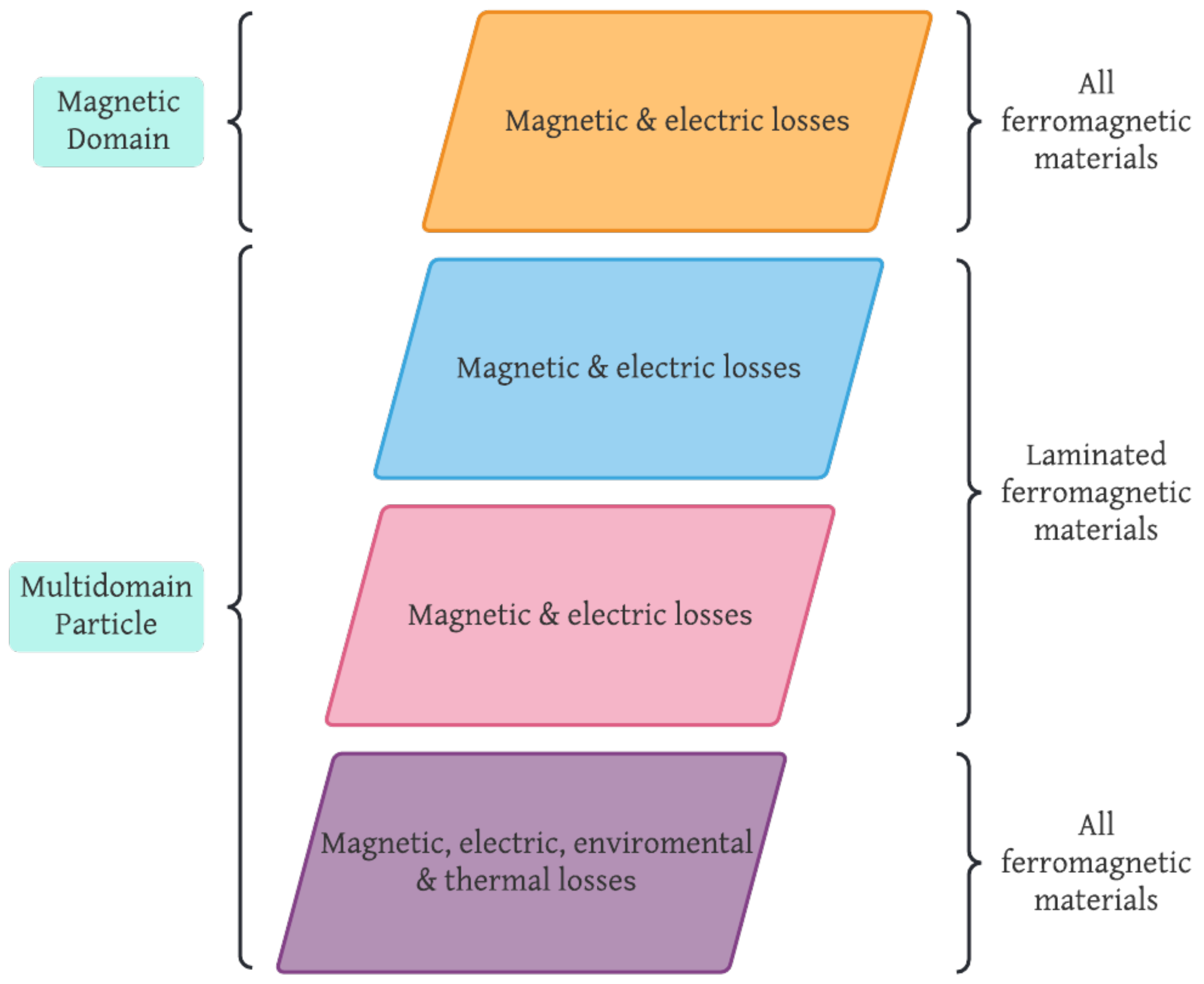
4. General Core Losses Models

In a magnetic component, the core is the key to determine its magnetic properties and performance [72]. So to achieve an optimal magnetic component’s performance, the core losses effects must be characterized [73].
Core loss depends on many aspects that must be considered [74,75]:
  • Relative permeability.
  • Magnetic saturation point.
  • Temperature operation range.
  • AC excitation frequency and amplitude.
  • Voltages’ waveform.
  • DC bias.
  • Magnetization process.
  • Peak-to-peak value of magnetic flux density.
In the case of the magnetization process, some factors are instantaneous values and time variation values. While to waveform’s topic, the duty ratio of the excitation waveform also influence the core loss [76,77].
Generally, the core loss is provided at a specific frequency and a maximum flux density [78]. The variation frequency effect in ferromagnetic materials is related to Eddy currents and the wall-domain displacement [72].
Core losses in ferrimagnetic and ferromagnetic materials are similar. Both have losses due to Eddy currents, hysteresis, and anomalous; however, there are differences concerning flux density, magnetization process, and hysteresis loop shape that define the magnetic behavior of each one.
The hysteresis is one of the principal features of ferromagnetic materials; it describes the internal magnetization of magnetic components as a function of external magnetizing force and magnetization history [79]. The source of hysteresis loss is the domain wall movement and the magnetic domains’ reorientations [80,81].
The hysteresis loss is defined as power loss in each cycle of magnetization and demagnetization into a ferromagnetic material [82]. If a magnetic sample is excited from zero to the maximum field value and later comes back at the initial field’s value, it will be observed that the power returned is lower than the supplied it [83,84].
The loss is proportional to the area surrounded by the upper and lower traces of the hysteresis curve; it represents the per cycle loss and it is proportional to f · B 2 [82]. However, if the curve’s shape remains equal for each successive excitation, the loss power will be the product of the core’s area and the applied frequency [80,82].
The hysteresis loops give a lot of information about the magnetic properties [72]. An accurate way to calculate core loss is by measuring the full hysteresis curve [85].
There are many methods to calculate core losses; Figure 3 shows a general classification. All of them are based on one, two, or three main effects (hysteresis, Eddy current, and anomalous); depending on the method’s focus they are analyzed as macro or micro phenomena. Each one of the methods shown in Figure 3 will be detailed in the following paragraphs.

4.1. Mathematical Models

Mathematical hysteresis modelling is divided into approaches based on the theory of micro-magnetics and the methods based on curve-fitting. The hysteresis models require complex computation to calculate the model parameters, the material parameter that manufacturers do not provide, or mathematical approximations where the accuracy depends on the number of data points to fit hysteresis loops [86,87]. These drawbacks remain if they are analyzed from a purely mathematical or a physical point of view [78].
The Preisach model and the Jiles-Atherton (J-A) model have been widely used in practical problems to calculate core loss, they are in continuous improvement, and they are considered a valuable and convenient tool to the hysteresis modelling [87,88,89].
The Preisach is a scalar-static model that considers several quantities of basic’s domain-walls [72]. It is an accurate-phenomenological model, such that it could describe any system that shows a hysterical behavior [87,90]. This model can be a link between theory and experimentation to describe a microscopical system by measuring macroscopic behavior [78].
Given a typical hysteresis loop for separate domains as shown in Figure 4, H d and H u are the switching magnetic fields “down” and “up”, respectively. The magnetization M ( t ) of a particle having the hysteresis loop m ^ ( H u , H d ) is described as the magnetic moment m s while the particle is switched up m ^ ( H u , H d ) H ( t ) = + m s or down m ^ ( H u , H d ) H ( t ) = m s [87]. It is assumed that all domains have a distribution of reversal fields H u and H d that can be characterized by a distribution function ϕ ( H u , H d ) , so the Preisach model is usually defined as:
M ( t ) = H u H d ϕ ( H u , H d ) m ^ ( H u , H d ) H ( t ) d H u d H d .
A drawback of the Preisach model is the several measurement data to adapt it to the B-H environment’s changes [72]. Nonetheless, it can track complex magnetization processes and minor loops [78].
On the other hand, the J-A model requires solving a strongly non-linear system of equations, with five scalar parameters, which are determined in an experimental way; this is, measuring the hysteresis loop [92]. This model predicts the major hysteresis loops under quasi-static conditions, besides there is a dynamic conditions version in which eddy current loss, DC-bias fields, anisotropy, and minor loops are included [86,93].
The J-A model is described as the sum of reversible M r e v and irreversible M i r r magnetizations, hence, the total magnetization M is:
M = M i r r + M r e v
d M r e v d H = c d M a n d H d M i r r d H
d M i r r d H = M a n M i r r δ x / μ 0 α i c ( M a n M i r r )
M a n = M s coth H e f f a s a s H e f f
H e f f = H + α i c M .
In these equations, c is the reversibility coefficient, α i c is the inter-domain coupling, δ indicates the direction for magnetizing field ( δ = 1 for the increasing field, and δ = 1 for decreasing field), x is the Steinmetz loss coefficient, M s is the saturation magnetization, M a n is anhysteretic magnetization, H e f f is the effective field, H is the magnetic field, μ 0 is the permeability in free-space, and a s is the shape parameter for anhysteretic magnetization [73]. A drawback of the J-A model is the computing time and the computing resources to solve a strongly non-linear system.
On the other hand, Eddy’s losses are produced due to changing magnetic fields inside the analyzed core. These fast changes generate circulating peak currents into it, in the form of loops, generating losses measured in joules [94].
These losses depend on the actual signal shape instead of only the maximum value of the density flux. The power loss is proportional to the area of the measured loops and inversely proportional to the resistivity of the core material [50,94].
Eddy currents are perpendicular to the magnetic field axis and domain at high-frequency, as well, they are proportional to the frequency. This phenomenon can be treated as a three-dimensional character or in a simplified way [95]. In a magnetic circuit, Eddy currents cause flux density changes in specific points of its cross-section [96].
One way to describe the Eddy currents distribution is based on Maxwell’s equations [95,97]. In practice, especially on higher frequencies, there is a difference in the measured total loss between the sum of the hysteresis loss and the Eddy current loss; this difference is known as anomalous or residual losses [13]. The effect of temperature and the relaxation phenomena are enclosed in this category [82].

4.2. Time-Domain Approximation Models

For the time-domain model, the loss separation method is used in the frequency domain, using Fast Fourier Transform (FFT) [13].
Time-domain approximation (TDA) can be used for sinusoidal and non-sinusoidal magnetic flux density; however, it is only valid for linear systems [98]. The losses are calculated considering each frequency, separately, and adding them later [85,98].
P c = n = 1 π ( f n ) B n H n sin ϕ n .
According to Equation (7), time-domain approximation is a function of the fundamental frequency f, the peak values of the nth harmonic of the magnetic field H and magnetic flux density B, and ϕ n the angle between B n and H n .
When a pulse width modulation (PWM) is induced in a magnetic component made with non-linear material, a non-sinusoidal ripple is generated [93]. Fourier’s core loss decomposition accuracy is not acceptable for non-sinusoidal flux densities and it is limited for frequencies > 400 Hz, as it was reported in [99].

4.3. Loss Separation Models

The loss separation method (LSM) is well-known, accurate and straightforward in many applications [94]. It defines the core loss ( P C ) under a dynamic magnetic excitation as the sum of three components: the hysteresis loss ( P h ), the Eddy current loss ( P e d d y ) and the residual or anomalous loss ( P a n o m ) [82] is given by:
P c = P h + P e d d y + P a n o m .
According to Equation (8), the power loss per unit volume is the sum of a hysteresis and dynamic contribution; Eddy currents and residual loss are part of the latest one [100].
The loss separation method was proposed in 1924 by Jordan, which describes the core losses as the sum of the hysteresis loss (or static loss) and the Eddy loss (or dynamic loss) [98]
P c = k h f B s + k e d d y f 2 B s 2 .
Years later, Bertotti extended Jordan’s proposal, adding an extra term to calculate residual losses. G. Bertotti is the maximum exponent in the loss separation methods; his theory provides a solid physical background. The total power loss can be calculated at any magnetizing frequency as the sum of three components [44]. This is show in the following equation
P c = k h f B s x + k e d d y f 2 B s 2 + k a n o m f 1.5 B s 1.5 ,
where k h , k c , k a n o m are the hysteresis, Eddy currents, and anomalous coefficients, respectively. The hysteresis coefficient decreases if the magnetic permeability increase. The frequency is represented by f, while x is the Steinmetz coefficient and has values between 1.5 and 2.5, according to the permeability of the material. Finally, B s is the peak value of the flux density amplitude [23,100].
From Equation (10), Bertotti defined eddy currents and anomalous losses in Equations (11) and (12), respectively, for lamination materials.
P e d d y = π 2 d 2 f 2 B s 2 ρ β
P a n o m = 8 G A V 0 ρ B s 1.5 f ,
where G is about 0.2, ρ is the electrical resistivity, d is the lamination thickness, A is the cross sectional area of the lamination, β is the magnetic induction exponent, G is a dimensionless coefficient of Eddy current, and V 0 is a parameter that characterizes the statistical distribution of the magnetic objects responsible for the anomalous eddy currents [101]. However, this method only provides average information, so it is not able to calculate core loss under harmonic excitation [94]. Still, it can calculate core loss under square waveforms considering DC bias [102].

4.4. Empirical Models

A big group of empirical models is based on a simple power-law equation, which was proposed in 1982 by Charles Steinmetz to calculate hysteresis loss without including the frequency relation [103]. This equation is known as the Steinmetz equation or original Steinmetz equation (OSE),
P OSE = k f α B s β ,
where P OSE is the time-average core loss per unit volume, B s the peak induction of the sinusoidal excitation, k is a material parameter, α , and β are the frequency and magnetic induction exponents, respectively, often referred to as Steinmetz parameters [76]. Typically α is a number between 1 and 2, and β is typically between 1.5 and 3 [104].
The Steinmetz parameters can be determined from a double logarithm plot by linear curve fitting of the measured core loss data. Therefore Equation (13) assumes only sinusoidal flux densities with no DC bias [76,77,98,105].
In modern power electronics applications, sinusoidal-wave voltage excitation is not practical because many of them, like power converters, require square-wave voltage excitation [106]. Therefore, a square waveform’s core loss can be lower than the sinusoidal-wave’s losses for the same peak flux density and the same frequency [76,107].
To overcome the aforementioned situation, modifications to OSE have been made. The result was the developing Modified Steinmetz Equation(MSE) [108], General Steinmetz Equation (GSE) [109], Doubly Improved Steinmetz Equation (Improved-Improved Steinmetz Equation, i 2 GSE) [110], Natural Steinmetz Equation (NSE) [85], and Waveform-Coefficient Steinmetz Equation (WcSE) [111]. It is important to mention that the OSEs’s constants α , β , and k remain in those expressions.
Modified Steinmetz Equation was the first modification proposed to calculate core loss with non-sinusoidal excitation, incorporating into OSE the influence of a magnetization rate. MSE is proposed in [112] as follows
P MSE = ( k f e q α 1 B s β ) f r
f e q = 2 Δ B 2 π 2 0 T d B ( t ) d t 2 d t ,
where f r is the periodic waveform fundamental frequency, f e q is the frequency equivalent, Δ B is the magnetic induction peak to peak, and d B ( t ) / d t is the core loss magnetization rate.
A drawback of Equation (14) is that its accuracy decreases with the increasing of waveform harmonics, and for waveforms with a small fundamental frequency part [77,85,113].
Another modification of OSE is the Generalized Steinmetz Equation to overcome the drawbacks of OSE and MSE for sinusoidal excitations, whose expression is:
P G S E = k 1 T 0 T d B ( t ) d t α B ( t ) β α d t
k 1 = k 2 β α ( 2 π ) α 1 0 2 π cos θ α sin θ ( β α ) d θ .
In this equation, the current value of flux is considered additional to the instantaneous value of d B ( t ) / d t , B ( t ) , T is the waveform period, and θ is the sinusoidal waveform phase angle. The main GSE’s advantage is it DC-bias sensitivity. However, its accuracy is limited if a higher harmonic part of the flux density becomes significant [85,98].
The Improved Generalized Steinmetz Equation is considered one of the best methods because it is a practical and accurate [114]. It is defined as follows:
P i GSE = k i T 0 T d B ( t ) d t α Δ B β α d t
k i = k 2 β α ( 2 π ) α 1 0 2 π cos θ α d θ .
Unlike GSE, which uses the instantaneous value B ( t ) , iGSE considers its peak-to-peak value Δ B . Any excitation waveform can be calculated by it; therefore, it has better accuracy with waveforms that contained strong harmonics [114,115,116,117].
The Natural Steinmetz Extension is similar approach to the iGSE; this means that Δ B was also taken into account [85,118]. It is written as:
P N S E = Δ B 2 β α k N T 0 T d B ( t ) d t α d t
k N = k ( 2 π ) α 1 0 2 π cos θ α d θ .
The NSE focuses on the impact of rectangular switching waveform like PWM, so Equation (17) can be modelled for a square waveform with duty ratio D by:
P N S E = k N ( 2 f ) α B s D 1 α + ( 1 D ) 1 α .
The Improved–Improved Generalized Steinmetz Equation (i 2 GSE) considers the relaxation phenomena effect in the magnetic material used due to a transition to zero voltage [115]. The i 2 GSE was developed to work with any waveform but its main application is with trapezoidal magnetic flux waveform [110]. For a trapezoidal waveform, i 2 GSE is described as follows:
P i 2 GSE = 1 T 0 T k i d B ( t ) d t α ( Δ B ) ( β α ) d t + l = 1 n Q r l P r l
P r l = k r T d d t B ( t ) α r ( Δ B ) β r ( 1 e t 1 τ )
Q r l = e q r d B ( t + ) / d t d B ( t ) / d t .
Note that P r l and Q r l calculate the variation of each voltage change and the voltage change, respectively. However, to use the i 2 GSE requires additional coefficients as can be seen in Equation (19) where k r , α r , β r , τ and q r are material parameters and they have to be measured experimentally; given that, they are not provided by manufacturers and the steps to extract the model parameters are detailed in [119]. The expression given by Equation (19) can also be rewritten by a triangular waveform.
Finally, the Waveform-Coefficient Steinmetz Equation (WcSE) was proposed in [111] to include the resonant phenomena, and it applies only at situations with certain loss characteristics. This empirical equation is used in high-power, and high-frequency applications, where resonant operations are adopted to reduce switching losses. The WcSE is a simple method that correlates a non-sinusoidal wave with a sinusoidal one with the same peak flux density; the waveform coefficient ( F W C ) is the ratio between the average value of both types of signals [119,120]. WcSE can be written as follows:
P WcSE = F W C k f α B s β .
The most important characteristics of each approximation based on the Steinmetz equation are listed in Table 1.
In addition to the methods listed before, in [110] the authors provided several graphs for different materials at different operating temperatures making use of the Steinmetz Premagnetization Graph (SPG), which is a simple form to show the dependency of Steinmetz’s parameters on premagnetization to calculate the core losses under bias conditions.
Using the SPG, the changes of Steinmetz in iGSE can be considered; it is also possible to calculate the core loss under any density flux waveform [19,74].

Empirical Core Losses Proposals

The primary purpose of this section is to show a few empirical core losses models proposals to emphasize the diversity of parameters that are taken into account: voltage waveforms, temperature effect, and the versatility of using them to calculate core losses.
Generally, square waveforms are used in power electronic applications resulting in triangular waveform induction and flux density; therefore, core losses models must contemplate this waveform. However, a sinusoidal approximation for a duty rate of 50 % is valid [121].
Curve fitting is used to approximate and characterize the model’s core losses parameters. Nonetheless, curve fitting by polynomials are unstable with minor changes at entry, resulting in a big variation on coefficients, so the designer must be meticulous in selecting the model as the curve fitting method and logarithm curve [121].
The Composite Waveform Hypothesis (CHW) was proposed in 2010; it is based on a hypothesis that establishes that if a rectangular waveform given is decomposed in two pulses, total core losses are the sum of the losses generated by each one of the two pulses [26,122]. This method is described by
P CHW = 1 T P s q r V 1 N , t t 1 + P s q r V 2 N , t t 2 ,
where P s q r is the power losses of a rectangular waveform with the parameters given, V 1 / N and V 2 / N are the voltage by turn in time t 1 and t 2 , respectively.
Villar’s proposal [120,123] calculates core losses for three-level voltage profiles through a lineal model by parts. Villar takes the models based on Steinmetz equations and modifies them by a linear model by parts (22), (23) and (24); this includes a duty ratio parameter in the original equations, getting expressions to calculate core losses for three-level voltage profiles.
P V i l l a r OSE = k f α B s β D β
P V i l l a r I GSE = 2 α + β k i f α B s β D β α + 1
P V i l l a r WcSE = π 4 1 + ω π k f α B s β D β .
In Equation (24) the parameter ω is the duration of zero-voltage period this is, power electronics converters’ switching devices take a short time to start their conduction mode; therefore, Villar includes this effect in its model by the flux density’s equation as follows:
B s = 1 2 U N A e f f T 2 T ω , T ω = ω T 2 π ,
where U is a DC constant voltage, A e f f is the core’s area effective, and T ω is the length of zero-voltage period.
Villar’s proposal also is applied to the equivalent elliptical loop (EEL); however, the proposal does not include thermal parameters.
Another alternative is the model proposed by Gorécki given by Equation (26) in [124,125], which includes 20 parameters. Those are divided into three groups: electrical parameters, magnetic parameters, and thermal parameters. At the same time, the magnetic parameters’ are subdivided into three groups: core material parameters, geometrical parameters, and ferromagnetic material parameters corresponding to power losses. The model parameters can be obtained by the datasheets of the cores and experimental way when the inductor is tested under specific conditions, which is called local estimation.
P G o r e c k i = P v 0 f α B s β ( 2 π ) α 1 + α p ( T R T M ) 2 0.6336 0.1892 ln α
P v 0 = α e x p f + f 0 f 3 + a 1 ( T R T M ) + a 2 e x p f f 2 f 1
β 2 1 e x p T R α T + 1.5 if e x p T R α T > 0 1.5 if e x p T R α T < 0 .
In these equations, T R is the core temperature, T M is the core temperature at which the core has a minor loss, α p is the losses’ temperature coefficient in ferromagnetic material, a, a 1 , a 2 , f 0 , f 1 , f 2 , f 3 , and α T are material parameters.
Gorecki’s model is also valid for the triangular waveform following Equation (27), where D is the duty ratio of the waveform.
P G o r e c k i = P v 0 f α B s β ( 2 π ) α 1 + α p ( T R T M ) 2 D ( 1 α ) + ( 1 + D ) ( 1 α ) .
The main drawback of Gorecki’s model is to find the overall parameters mentioned before, and solving the equations related to the power core losses.

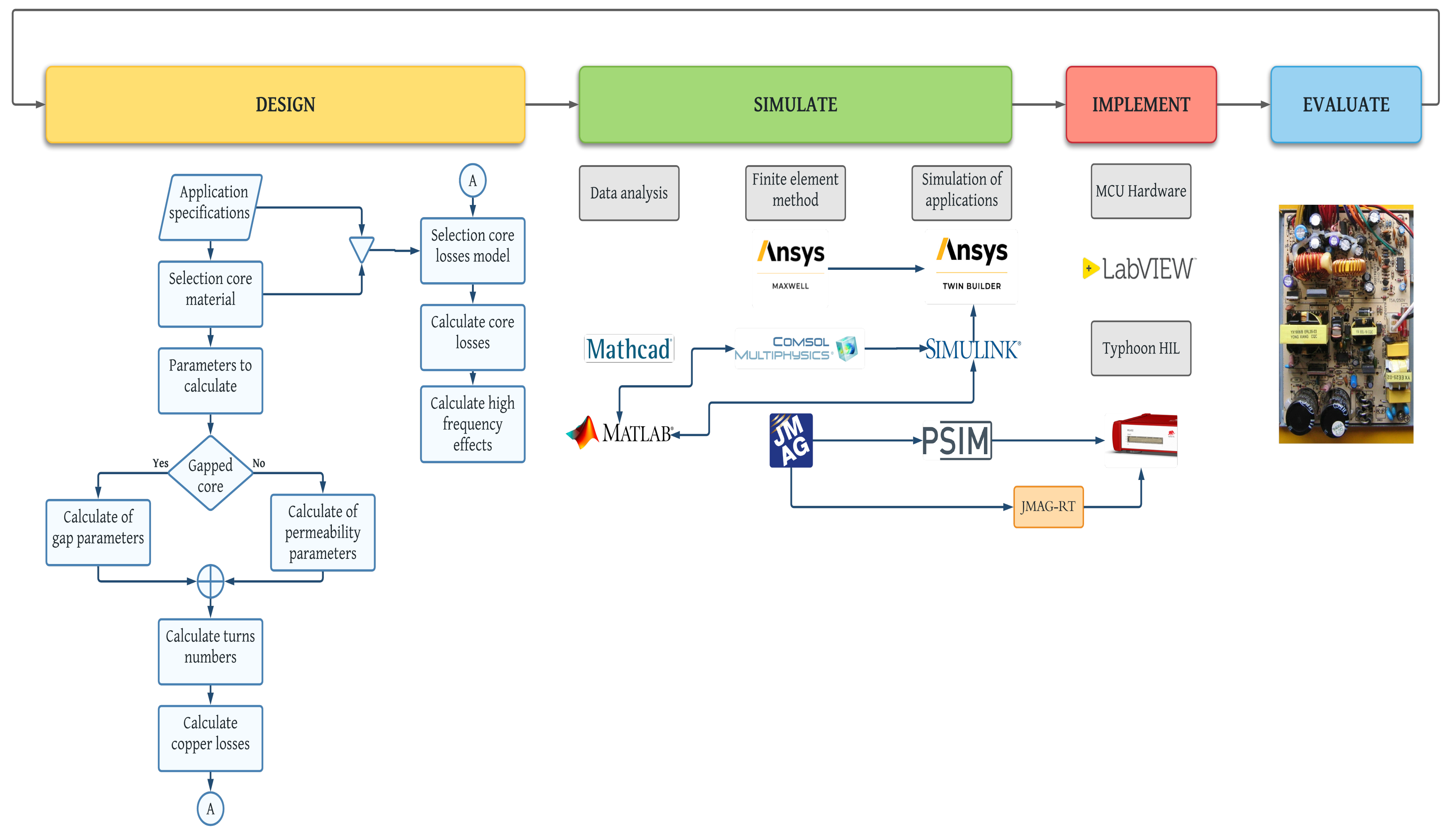
5. Simulation Software

Several core loss models have been reviewed; they are the base for developing a series of numerical and theoretical models that are useful for designing magnetic components. Nonetheless, they fail to predict dynamic magnetic behaviors. Usually, the calculation of the core parameters’ losses in a dynamic situation is complicated (specially with complex geometries), and it requires a rigorous numerical treatment [126].
Several methods are used in the simulation and calculation of core and wire windings. However, the finite element method (FEM) is the most widely used for designs in 2-D and 3-D [22].
In 1960 Clough introduced the name of Finite Element Method (FEM), which continues to these days [127]. FEM is a computational method whose basic idea consists on finding a complicated problem and replacing it with a simpler one. It is always possible to improve the approximation solution spending more computational effort [127,128].
To find the solution of a region, the FEM considers that it is built of many small, interconnected subregions called elements [128], and the global solution is obtained from the union of individual solutions on these regions [129].
The FEM is a tool for solving problems with partial differential equations that are part of physics problems [130]. FEM has quite benefits of using it; some of them is the freedom that it offers in the discretization’s selection, and its well developed theoretical base that allows valid error estimates for the numerical model equations, and its flexibility to be adapted to a wide range of numerical problems [129,131].
The FEM was originally developed to solve problems in solid-state mechanics. Still, its versatility, excellent simulation technique, availability to optimize the mesh size, and accuracy have been implemented in a wide variety of applied science and engineering [127,129].
Mathematical models are discretized by FEM, resulting in numerical models. To solve the discretized equations, Finite Element Analysis (FEA) is used [131,132].
There are many FEM software developers in the market; however, Ansys® is the leader so far. Ansys, Inc. (Canonsburg, PA, USA) was founded in 1970s, and since then, it has developed, commercialized and brought support at several range of physics through engineering simulation software. The Ansys® catalogue includes simulation software for semiconductors, structures, materials, fluids, and electronics.
An exciting tool that Ansys has developed in recent years is Twin Builder®, a multi-technology platform to create digital representations simulations, recollected real-time data information through sensor inputs asset with real-world [133]. Twin Builder® is a powerful and robust multi-domain system modelling compatible with a series of standard languages and formats as SPICE, Python, C/C++, simplorer modelling language (SML), among others. It can be used to develop basic simulation experiments and advanced simulation studies, from 2-D and 3-D physics simulations. Inclusive the functional mock-up interface (FMI standard) can import and export models as available mockup units (FMU). An example of an electromagnetic digital twin is shown in Figure 5. Twin Builder® only is compatible with Ansys software and its main application is in the industry as virtual laboratory to test any kind of system.
Added to these FEM software developers, there is Comsol Multiphysics®, which is a powerful software tool for developing and simulating modelling designs in all fields of engineering, manufacturing, and scientific research [134]. This software was founded in 1986. Its main characteristic is its friendly graphical user interface. The Comsol Multiphysics® community is more significant than the other software. In Figure 6, two simulations are provided. Comsol Multiphysics® can import designs in CAD and export final designs to Simulink®, given that both belong to the MathWorks® family. Comsol Multiphysics® is oriented to students and academic researchers, it is not complex to learn and it is an excellent option to start with for FEM software.
Another big company of FEM software is JMAG®, a simulation software specialized for electric device design and development, including the accurate model of complex magnetic phenomena. It was founded in 1983, and currently, its most attractive feature is the capability to link various systems through its interface [135].
The JMAG® interface allows the data exchange at high speed without loss of precision with other software as SPEED, PSIM and MATLAB/Simulink; one example of this software is shown in Figure 7. Additionally, JMAG® allows to the user import and export multi-purpose files and to run VB Script and other scripting languages [135].
Another feature of JMAG® is its CAD interface to link and import files with software as SOLIDWORKS, CATIA V5, among others to test the model developed using software in the loop (SIL), model in the loop (MIL) and hardware in the loop (HIL) systems, which are applied for system-level and real-time simulations [135,136]. JMAG® is a specialized software to model inductors and magnetic motors adding vibration and thermal analysis; however, the information about it is limited, and it is complex to learn.
The software mentioned before are the most commonly used; however, there are many other finite element software packages available to any platform and they have different features [137].

6. Magnetic Components Design Process

In general, the design process of a magnetic component consists of four steps: design, simulate, implement, and evaluate Figure 8.
The design step can completely follow the diagram shown in Figure 8, where the application specifications will determine the selection core material up to the copper losses, the core losses model, and the high-frequency effects according to [139,140].
It is worth to mention, that there are some intermediate steps, which are related to core physical and magnetic parameters such as the cross section of the core, section of the core, length of it, effective relative permeability, peak to peak density ripple, among others [141]. In the same way, choosing a gapped core (a core with a concentrated air gap) instead of a distributed air gap core will impact its behavior and parameters to calculate; for the first one, gap parameters as length are a priority. For the second one, permeability parameters will be taken into account [142].
As applications specifications as selection core material are fundamental to select or design a core losses model, both will establish the minimum parameters to calculate power losses.
The simulate step is the masterpiece to validate the magnetic component designed, but at the same time, it will be a problematic step if the designer is not careful; FEM software always will give a solution but does not mean that it is correct. In a general way, simulation steps can be subdivided into three parts: data analysis, finite element method, and simulation of applications.
From the design steps depending on the models selected to calculate power losses, core physical parameters, and data related to the windings, many formulas are involved, and sometimes some depend on others; software such as Mathcad® and Matlab® are of great help in these cases. FEM is a big world, as it was explained in the section before. Once the magnetic component’s design is complete (windings and core parameters) and validated in FEM; the next step consists in exporting the final FEM design to software like Simulink® or Twin Builder®, PSIM®, to simulate it in a specific application and corroborate its correct performance [59,143,144,145,146].
The implementation step tests the simulated application through the interconnection of different sorts of software and platforms (MCU hardware, LabVIEW®, Typhoon HIL, among others) to simulate it with high fidelity, in similar conditions to real [147]. Typhoon HIL is a feasible example of this, as it can see in Figure 8. The reader interested in magnetic component testing is referred to [148,149,150,151,152,153] and the references therein.
The last one is to evaluate, that is, physically build the magnetic component designed and tested in the steps before and implement it in a circuit. Technically speaking, the tests obtained in the implementation step must coincide with the physical circuit measurements with a minimal error percentage. If the magnetic component behavior is not satisfactory, the steps must be repeated, modifying the necessary parameters until the desired results are obtained.

7. Magnetic Devices and Miniaturization

Transportation, electrification, medical applications, micromachines, wireless communication and wireless charging are some areas demanding new technology to develop compact and high performance applications; and the manufacturing of low losses magnetic components is key [154].
Magnetic components exhibit design difficulties when power conversion systems require low power levels and high frequencies due to the nonlinear behavior of magnetic materials, thermal limits, and the exponential increase of losses under these conditions.
Core data and core losses models are critical to design magnetic components properly and select the size of magnetic devices. According to core selection material different procedures may be applied [155].
Miniaturization of magnetic components and micromachines are an interesting couple to develop and implement in biomedical devices and applications. In biomedical applications magnetism-based systems are widely utilized, for example, to study and measure human tissue and organs (such as magnetocardiography, magnetoneurography, magnetoencephalography, and magnetomyography) [156,157,158,159]. By 2021, the market of magnetic sensors will worth around $7.6 billion due to their attractive commercial purposes and new application areas [160]. However, the development of efficient magnetic technologies that are sensitive, inexpensive, biocompatible and miniaturized is still far away [161].
The miniaturization, feasibility and integration of magnetic sensors for biomagnetic signal detection have been in constant evolution in terms of size, sensing signals magnitude (pico-Tesla scale), and environment conditions. In magnetic sensors, the magnetic field is converted into measurable quantities as voltage and current [156]. Some examples of them are the thin-film magnetoelectric (ME) sensors, optically pumped magnetometers (OPM), superconducting quantum interference device (SQUID), flux gate sensors, giant magnetoimpedance (GMI) sensor, magnetic sensors based on the thin-film magnetoresistive (MR), and conventional superconducting coils. Those are compared in Table 2 [156,160].
In [162], a GMI miniaturized magnetic sensor fabricated with a Co-based amorphous by Micro-Electro-Mechanical System (MEMS) technology wire is described, achieving a size of 5.6 × 1.5 × 1.1 mm 3 . Co-based amorphous wire is selected for its high impedance change rate, increasing the sensitive of the GMI sensor, it is used to fabricated a pick-up coil of 200 turns and diameter of 200 μ m.
A common problem in biomagnetic sensors is the noise at low frequencies, specifically between 10 and 100 Hz due to the small magnitude of measured signals. A set of bi-planar electromagnetic coils is a recent technique to cancelling the Earth’s noise nearby the magnetic sensors and improving their sensitivity [156].
Magnetic signal detection including portable and handled devices in the point-of-care testing (POCT) including mini magnetic induction coils and electromagnets to do the devices more portable, flexible and with high detection capabilities. In [163] several examples of these applications are described, where magnetic devices have dimensions in centimeters scale and those consider other POCT techniques for their favorable accuracy, high reliability, innovation and novelty, although their cost might increase.
Portable and small size, or even single handled devices that provide rapid and accurate detection have potential application of POCT [163]. Portable and wearable biosensors are the future of healthcare sensor technologies. Those have demonstrated their utility in disease diagnosis with accurate prediction. Their incorporation with mobile phones is known as digital health or mobile health, which promises reduce the frequency of clinical visits, prevent health problems and revolutionary the demand of micro and wearable sensors technology [164,165,166].
The emerge of microrobots and the use of a magnetic resonance imaging help to improve diagnostic capabilities by minimally invasive procedures. A microrobot is a robot on a microscale that can perform high-precision operations. Microrobots’ actuation system require input energy to act it, which usually requires special materials (soft and hard magnetic materials) or structural design (arrangement of coils) [167,168]. While the propulsion of microrobots, ferromagnetic cores and magnetic structures can be used to generate an image of many sites in the human body [169,170,171].
In [172], microcoils with a diameter < 1 mm are used to harvest electromagnetic energy wirelessly by inductive coupling in the on-board energy robots, achieving several milliwatts of power, capable of controlled motion and actuation with a maximum efficiency of 40%. This has been a recent development to controlled and powered remotely a system-engineered miniaturized robot (SEMER).
To increase the adaptability and robustness of robotic systems in challenging environments, and inter disciplinary research is needed, including material science, biology, control, among others [172]. Magnetic materials and magnetoelectric concepts of micro and nanorobots in magnetic applications are detailed in [173].
In this authors opinion the versatility, scalability, and flexibility of developing a power core loss model to analyze and allowing a better comprehension of the magnetic phenomena in ferromagnetic materials, will be the first step to the miniaturization of magnetic devices and power conversion systems at any scale [174,175].

8. Discussion

Nowadays, there are several models for studying, predicting, and analyzing the power losses in the ferromagnetic cores of magnetic components. Usually, these models consider a series of parameters based on magnetic units and frequency to predict and calculate power losses. Figure 9 illustrates a comparison between core losses models depending several features.
Nevertheless, one main application of magnetic components is in power electronics, where the measurement units are electric, which in many cases cause inexactness while designing a magnetic element. A common idea in the literature is that in a magnetic component with high operating frequency, its losses and size will be lower; however, this is not always true. There are many factors involved (kind of material, core losses, copper losses, among others) to determine the integrity of this expression. Although the last years’ power electronic researchers have been working hard to find and develop numerous techniques to achieve better performance from magnetic components, the way is still long. For instance, the future design of magnetic components should take advantage of all capabilities of the final application (support multiple input/outputs, multiple voltage/current domains, characterization of the material, losses’ reduction, among others), with the option to work in parallel with switches at high frequency [12,176].
On the other hand, the industry of FEM software is more versatile each year; several applications and tools are added to these, improving accuracy, functionality, scenarios to apply it, and user friendly environments. Nonetheless, a common point is a lack of compatibility among those, limiting the use of platforms to validate and complement the final design. This lack of compatibility motivates users to know different packages to solve a unique problem.
This is translated into a monetary cost to purchase different licenses and increase computer resources. Therefore, to motivate and improve the FEM designs, in this authors opinion, a standard format type should be implemented in the following years between those kinds of software to take advantage of each characteristic and unify all FEM files.
In the literature, static or dynamic core losses models can be found, depending on the designer choice, the loses calculus could be as complex as the model chosen [177]. So, the model selection in function of the material and the requirements’ application of a magnetic component’s design process are fundamental to achieving an accurate core losses calculus.
Table 3 illustrates a comparison between power core losses models, ferromagnetic materials, and accuracy. It is essential to mention that ferrite is the start point to validate any power core losses model, so this is not listed. Nonetheless, to the best authors knowledge, not all models had been tested in all ferromagnetic materials, or those are not suitable to calculate their power core losses.
Designers can use the information mentioned in Table 3 and Figure 9 to improve some of the power core loss models listed before or propose their model, always keeping in mind that any design parameter will be sacrificed to improve another one; magnetic components size will be reduced with frequency increment.
Due to the high energy consumption worldwide, renewable energy sources and energy efficiency have accelerated research in energy applications, conversion, transportation, and telecommunication [178]. Magnetic materials are the key piece of those research fields, mainly for their potential for energy efficiency and their impact on consumption power [179]. Materials’ demand as electric steel, iron, and cobalt will be exponential growth for 2026. Studies on the effect of magnetic materials in renewable energy have to be a priority to guarantee the supply chain, options for recycling, the footprint impact, the blueprint impact, and the socio-economical impact of their extraction [180,181].

9. Conclusions

In the literature, many core-losses models are available to select. Researchers continue developing new core losses models with specific features (core material, waveform, density flux, application, frequency range, among others), but the majority are not easy to replicate.
To develop a power core losses model that involves electrical, magnetic, thermal effects, suitable for all kinds of ferromagnetic materials, and also competent to power electronic is fundamental. Not only for advantages to calculate power core losses accurately but not to reach optimal magnetic components. The challenge is to understand the comportment of the magnetic materials and model them differently than ferrite magnetic elements because, until now, both are very similar, although their behaviour is quite different.
Each of the core losses models in this document is a point of start for researchers. Despite promising results using Steinmetz’s equations, those are not enough to calculate the core losses accuracy according to the need for the power electronic community. FEM software is indispensable nowadays to validate the power losses model as the magnetic component design. At the same time, virtual laboratories are promising to be the trend in a few years, allowing a reduction of the cost of a physical test bench to that of a virtual one and getting good approximations of the magnetic component behavior in a real environment. In addition, the option to interconnect different kinds of software to implement complete power electronics systems in platforms such as HIL, SIL, and MIL, makes the capability of design more versatile.

Author Contributions

Conceptualization, D.R.-S. and F.J.P.-P.; methodology, M.A.R.-L.; software, I.A.-V.; validation, J.P.-O., A.-I.B.-G. and F.J.P.-P.; formal analysis, M.A.R.-L.; investigation, D.R.-S.; resources, F.J.P.-P., and A.-I.B.-G.; data curation, J.P.-O.; writing original draft preparation, D.R.-S.; writing—review and editing, D.R.-S., M.A.R.-L., J.P.-O. and F.J.P.-P.; visualization, D.R.-S.; supervision, I.A.-V.; project administration, A.-I.B.-G.; funding acquisition, F.J.P.-P. and I.A.-V. All authors have read and agreed to the published version of the manuscript.

Funding

The authors thank Tecnológico Nacional de México, Instituto Tecnológico de Celaya. The work of Daniela Rodriguez-Sotelo was supported by CONACYT through a Ph.D. grant.

Acknowledgments

The authors thank IPN, Tecnológico Nacional de México, Instituto Tecnológico de Celaya and CONACYT.

Conflicts of Interest

The authors declare no conflict of interest.

Abbreviations

The following abbreviations are used in this manuscript:
P c Core loss P h Hysteresis or static loss
P e d d y Eddy current loss P a n o m Anomalous or residual loss
k h Hysteresis coefficient k e d d y Eddy currents coefficient
k a n o m Anomalous coefficientfFundamental frequency
BMagnetic flux density ϕ n Angle between B n and H n
B n Magnetic flux density of the nth harmonic H n Magnetic field of the nth harmonic
B s Magnetic induction peakxSteinmetz coefficient
dLamination thickness ρ Electrical resistivity
ACross-sectional area lamination f e q Equivalent frequency
M a n Anhysteretic magnetization α i c Inter-domain coupling
Δ B Magnetic induction peak to peak d B ( t ) / d t Core loss magnetization rate
β Magnetic induction exponent α Frequency exponent
δ Magnetizing field direction f r Fundamental frequency
θ Sinusoidal waveform phase angleTWaveform period
DDuty ratioNNumber of turns
F W C Waveform coefficient V 1 , V 2 Voltage
tTime ω Zero-voltage period duration
UDC constant voltage T ω Length of zero-voltage period
T M Core temperature with smallest losses T R Core temperature
MTotal magnetizationHMagnetic field
H e f f Effective magnetic field μ 0 Free-space permeability
M i r r Irreversible magnetization M r e v Reversible magnetization
A e f f Effective core area α p Losses temperature coefficient
B ( t ) Instantaneous value of core loss magnetization rate V 0 Magnetic objects statistical distribution
GEddy current dimensionless coefficient a s Anhysteretic magnetization shape parameter
M ( t ) Instantaneous magnetization M s  Saturation magnetization
m s Magnetic moment H ( t )  Instantaneous magnetic field
P s q r Rectangular waveform power lossesc Reversibility coefficient
k r , α r , β r , τ , q r
a, a 1 , a 2 , f 0 , f 1 ,Material parameters
f 2 , f 3 , α T , k

References

  1. Lee, H.; Jung, S.; Huh, Y.; Lee, J.; Bae, C.; Kim, S.J. An implantable wireless charger system with ×8.91 Increased charging power using smartphone and relay coil. In Proceedings of the IEEE Wireless Power Transfer Conference (WPTC), San Diego, CA, USA, 1–4 June 2021; pp. 1–4. [Google Scholar] [CrossRef]
  2. Yu, W.; Hua, W.; Zhang, Z. High-frequency core loss analysis of high-speed flux-switching permanent magnet machines. Electronics 2021, 10, 1076. [Google Scholar] [CrossRef]
  3. Pérez, E.; Espiñeira, P.; Ferreiro, A. Instrumentación Electrónica; Acceso Rápido; Marcombo: Barcelona, Spain, 1995. [Google Scholar]
  4. Chitode, J.; Bakshi, U. Power Devices and Machines; Technical Publications: Maharashtra, India, 2009. [Google Scholar]
  5. López-Fernández, X.; Ertan, H.; Turowski, J. Transformers: Analysis, Design, and Measurement; CRC Press: Boca Raton, FL, USA, 2017. [Google Scholar]
  6. Muttaqi, K.M.; Islam, M.R.; Sutanto, D. Future power distribution grids: Integration of renewable energy, energy storage, electric vehicles, superconductor, and magnetic bus. IEEE Trans. Appl. Supercond. 2019, 29, 3800305. [Google Scholar] [CrossRef] [Green Version]
  7. Phan, H.P. Implanted flexible electronics: Set device lifetime with smart nanomaterials. Micromachines 2021, 12, 157. [Google Scholar] [CrossRef] [PubMed]
  8. Ivanov, A.; Lahiri, A.; Baldzhiev, V.; Trych-Wildner, A. Suggested research trends in the area of micro-EDM—Study of some parameters affecting micro-EDM. Micromachines 2021, 12, 1184. [Google Scholar] [CrossRef]
  9. Kozai, T.D.Y. The history and horizons of microscale neural interfaces. Micromachines 2018, 9, 445. [Google Scholar] [CrossRef] [Green Version]
  10. Rashid, M.H. Power Electronics Handbook; Elsevier: Amsterdam, The Netherlands, 2018; p. 1510. [Google Scholar] [CrossRef]
  11. Matallana, A.; Ibarra, E.; López, I.; Andreu, J.; Garate, J.; Jordà, X.; Rebollo, J. Power module electronics in HEV/EV applications: New trends in wide-bandgap semiconductor technologies and design aspects. Renew. Sustain. Energy Rev. 2019, 113, 109264. [Google Scholar] [CrossRef]
  12. Hanson, A.J.; Perreault, D.J. Modeling the magnetic behavior of n-winding components: Approaches for unshackling switching superheroes. IEEE Power Electron. Mag. 2020, 7, 35–45. [Google Scholar] [CrossRef]
  13. Bahmani, A. Core loss evaluation of high-frequency transformers in high-power DC-DC converters. In Proceedings of the Thirteenth International Conference on Ecological Vehicles and Renewable Energies (EVER), Monte Carlo, Monaco, 10–12 April 2018; pp. 1–7. [Google Scholar] [CrossRef]
  14. Hossain, M.Z.; Rahim, N.A.; Selvaraj, J. Recent progress and development on power DC-DC converter topology, control, design and applications: A review. Renew. Sustain. Energy Rev. 2018, 81, 205–230. [Google Scholar] [CrossRef]
  15. Silveyra, J.M.; Ferrara, E.; Huber, D.L.; Monson, T.C. Soft magnetic materials for a sustainable and electrified world. Science 2018, 362, eaao0195. [Google Scholar] [CrossRef] [Green Version]
  16. Zurek, S. Characterisation of Soft Magnetic Materials under Rotational Magnetisation; CRC Press: Boca Raton, FL, USA, 2017; p. 568. [Google Scholar]
  17. Cullity, B.; Graham, C. Soft magnetic materials. In Introduction to Magnetic Materials; John Wiley & Sons, Ltd.: Hoboken, NJ, USA, 2008; Chapter 13; pp. 439–476. [Google Scholar] [CrossRef]
  18. Krishnan, K.M. Fundamentals and Applications of Magnetic Materials; Oxford University Press: Oxford, UK, 2016; p. 816. [Google Scholar] [CrossRef]
  19. Islam, M.R.; Rahman, M.A.; Sarker, P.C.; Muttaqi, K.M.; Sutanto, D. Investigation of the magnetic response of a nanocrystalline high-frequency magnetic link with multi-input excitations. IEEE Trans. Appl. Supercond. 2019, 29, 0602205. [Google Scholar] [CrossRef]
  20. Dobrzanski, L.A.; Drak, M.; Zieboqicz, B. Materials with specific magnetic properties. J. Achiev. Mater. Manuf. Eng. 2006, 17, 37. [Google Scholar]
  21. Duppalli, V.S. Design Methodology for a High-Frequency Transformer in an Isolating DC-DC Converter. Ph.D. Thesis, Purdue University, West Lafayette, IN, USA, 2018. [Google Scholar]
  22. Liu, X.; Wang, Y.; Zhu, J.; Guo, Y.; Lei, G.; Liu, C. Calculation of core loss and copper loss in amorphous/nanocrystalline core-based high-frequency transformer. AIP Adv. 2016, 6, 055927. [Google Scholar] [CrossRef] [Green Version]
  23. Balci, S.; Sefa, I.; Bayram, M.B. Core material investigation of medium-frequency power transformers. In Proceedings of the 2014 16th International Power Electronics and Motion Control Conference and Exposition, Antalya, Turkey, 21–24 September 2014; pp. 861–866. [Google Scholar]
  24. de Sevilla Galán, J.F. Mejora del Cálculo de las Pérdidas por el Efecto Proximidad en alta Frecuencia Para Devanados de Hilos de Litz. Available online: https://oa.upm.es/56807/1/TFG_JAVIER_FERNANDEZ_DE_SEVILLA_GALAN.pdf (accessed on 24 February 2022).
  25. Herbert, E. User-Friendly Data for Magnetic Core Loss Calculations. Technical Report 4. 2008. Available online: https://www.psma.com/coreloss/eh1.pdf (accessed on 24 February 2022).
  26. Sullivan, C.R.; Harris, J.H.; Herbert, E. Testing Core Loss for Rectangular Waveforms the Power Sources Manufacturers Association. Technical Report 973. 2010. Available online: https://www.psma.com/coreloss/phase2.pdf (accessed on 24 February 2022).
  27. Tacca, H.; Sullivan, C. Extended Steinmetz Equation; Report of Posdoctoral Research; Thayer School of Engineering: Hanover, NH, USA, 2002. [Google Scholar]
  28. Ulaby, F.T. Fundamentos de Aplicaciones en Electromagnetismo; Pearson: London, UK, 2007. [Google Scholar]
  29. Cheng, D. Fundamentos de Electromagnetismo para Ingeniería. Mexicana, A., Ed.; 1997; Available online: https://www.academia.edu/36682331/Fundamentos_de_Electromagnetismo_para_Ingenieria_David_K_Cheng (accessed on 24 February 2022).
  30. Coey, J.M.D. Magnetism and Magnetic Materials; Cambridge University Press: Cambridge, UK, 2010. [Google Scholar] [CrossRef] [Green Version]
  31. Goldman, A. Handbook of Modern Ferromagnetic Materials; Springer: Boston, MA, USA, 1999. [Google Scholar] [CrossRef]
  32. Gupta, K.; Gupta, N. Magnetic Materials: Types and Applications. In Advanced Electrical and Electronics Materials; John Wiley & Sons, Ltd.: Hoboken, NJ, USA, 2015; Chapter 12; pp. 423–448. [Google Scholar] [CrossRef]
  33. Hitachi. Nanocrystalline Material Properties; Hitachi: Tokyo, Japan, 2019. [Google Scholar]
  34. County Council, K.; Richardson, A. Silver Wire Ring. 2017. [image/JPEG]. Available online: https://www.academia.edu/2306387/With_Dickinson_T_M_and_Richardson_A_Early_Anglo_Saxon_Eastry_Archaeological_Evidence_for_the_Beginnings_of_a_District_Centre_in_the_Kingdom_of_Kent_Anglo_Saxon_Studies_in_Archaeology_and_History_17 (accessed on 24 February 2022).
  35. Alisdojo. Detail of an Enamelled Litz Wire. 2011. [image/JPEG]. Available online: https://commons.wikimedia.org/wiki/File:Enamelled_litz_copper_wire.JPG (accessed on 24 February 2022).
  36. Magnetics. Powder Cores Properties; Magnetics: Pittsburgh, PA, USA, 2019. [Google Scholar]
  37. Laboratory, N.E.T. FINEMET Properties. 2018. Available online: https://www.hitachi-metals.co.jp/e/products/elec/tel/p02_21.html#:~:text=FINEMET%C2%AE%20has%20high%20saturation,and%20electronics%20devices%20as%20well (accessed on 24 February 2022).
  38. CATECH®. Amorphous and Nanocrystalline Core; CATECH: Singapore, 2022. [Google Scholar]
  39. Soon, H. Wire. 2017. [image/JPEG]. Available online: https://iopscience.iop.org/article/10.1088/1742-6596/871/1/012098/pdf (accessed on 24 February 2022).
  40. Aluminium Wire, 16 mm2. 2012. [image/JPEG]. Available online: https://ceb.lk/front_img/specifications/1540801489P.V_.C_._INSULATED_ALUMINIUM_SERVICE_MAIN_WIRE-FINISHED_PRODUCT_.pdf (accessed on 24 February 2022).
  41. County Council, K.; Richardson, A. Length of Gold Wire, Ringlemere. 2017. [image/JPEG]. Available online: https://www.sachsensymposion.org/wp-content/uploads/2012/04/68th-International-Sachsensymposion-Canterbury.pdf (accessed on 24 February 2022).
  42. SpinningSpark. Transformer Core. 2012. [image/JPEG]. Available online: https://commons.wikimedia.org/wiki/File:Transformer_winding_formats.jpg (accessed on 24 February 2022).
  43. TheDigitalArtist. coil-gd137ed32f-1920. 2015. [image/JPEG]. Available online: https://plato.stanford.edu/entries/digital-art/ (accessed on 24 February 2022).
  44. Fiorillo, F.; Bertotti, G.; Appino, C.; Pasquale, M. Soft magnetic materials. In Wiley Encyclopedia of Electrical and Electronics Engineering; American Cancer Society: Atlanta, GA, USA, 2016; pp. 1–42. [Google Scholar] [CrossRef]
  45. Aguglia, D.; Neuhaus, M. Laminated magnetic materials losses analysis under non-sinusoidal flux waveforms in power electronics systems. In Proceedings of the 15th European Conference on Power Electronics and Applications (EPE), Lille, France, 2–6 September 2013; pp. 1–8. [Google Scholar] [CrossRef] [Green Version]
  46. McLyman, C. Transformer and Inductor Design Handbook, 3rd ed.; Taylor & Francis: Abingdon-on-Thames, UK, 2004. [Google Scholar]
  47. Tsepelev, V.; Starodubtsev, Y.; Konashkov, V.; Belozerov, V. Thermomagnetic analysis of soft magnetic nanocrystalline alloys. J. Alloys Compd. 2017, 707, 210–213. [Google Scholar] [CrossRef]
  48. Ouyang, G.; Chen, X.; Liang, Y.; Macziewski, C.; Cui, J. Review of Fe-6.5 wt% silicon steel-a promising soft magnetic material for sub-kHz application. J. Magn. Magn. Mater. 2019, 481, 234–250. [Google Scholar] [CrossRef]
  49. Yuan, W.; Wang, Y.; Liu, D.; Deng, F.; Chen, Z. Impacts of inductor nonlinear characteristic in multi-converter microgrids: Modelling, analysis and mitigation. IEEE J. Emerg. Sel. Top. Power Electron. 2020, 8, 3333–3347. [Google Scholar] [CrossRef]
  50. Kazimierczuk, M. High-Frequency Magnetic Components, 2nd ed.; John Wiley & Sons, Ltd.: Hoboken, NJ, USA, 2013. [Google Scholar] [CrossRef]
  51. Tumanski, S. Handbook of Magnetic Measurements; Series in Sensors; CRC Press: Boca Raton, FL, USA, 2016. [Google Scholar]
  52. Goldman, A. Magnetic Components for Power Electronics; Springer: Berlin/Heidelberg, Germany, 2012. [Google Scholar]
  53. Wang, Y.; Calderon-Lopez, G.; Forsyth, A. Thermal management of compact nanocrystalline inductors for power dense converters. In Proceedings of the IEEE Applied Power Electronics Conference and Exposition (APEC), San Antonio, TX, USA, 4–8 March 2018; pp. 2696–2703. [Google Scholar] [CrossRef]
  54. Conde, C.; Blázquez, J.; Conde, A. Nanocrystallization process of the Hitperm Fe-Co-Nb-B alloys. In Properties and Applications of Nanocrystalline Alloys from Amorphous Precursors; Idzikowski, B., Švec, P., Miglierini, M., Eds.; Springer: Dordrecht, The Netherlands, 2005; pp. 111–121. [Google Scholar]
  55. Tsepelev, V.S.; Starodubtsev, Y.N. Nanocrystalline soft magnetic iron-based materials from liquid state to ready product. Nanomaterials 2021, 11, 108. [Google Scholar] [CrossRef]
  56. Lidow, A. Accelerating adoption of magnetic resonant wireless power based on the AirFuel, 2021. IEEE Wirel. Power Week. 2021. Available online: https://airfuel.org/wireless-power-week-2021-highlights/ (accessed on 24 February 2022).
  57. Jafari, M.; Malekjamshidi, Z.; Zhu, J. Copper loss analysis of a multiwinding high-frequency transformer for a magnetically-coupled residential microgrid. IEEE Trans. Ind. Appl. 2019, 55, 283–297. [Google Scholar] [CrossRef]
  58. Slionnnnnn. The Prototype of the Balanced Twisted Winding CM Choke. 2017. [image/JPEG]. Available online: https://en.wikipedia.org/wiki/File:4ffffss123.jpg (accessed on 24 February 2022).
  59. Corti, F.; Reatti, A.; Lozito, G.M.; Cardelli, E.; Laudani, A. Influence of non-linearity in losses estimation of magnetic components for DC-DC converters. Energies 2021, 14, 6498. [Google Scholar] [CrossRef]
  60. Zhu, F.; Yang, B. Power Transformer Design Practices; CRC Press: Boca Raton, FL, USA, 2021. [Google Scholar]
  61. Glisson, T. Introduction to Circuit Analysis and Design; Springer: Berlin/Heidelberg, Germany, 2011. [Google Scholar]
  62. Wang, W.; Nysveen, A.; Magnusson, N. The influence of multidirectional leakage flux on transformer core losses. J. Magn. Magn. Mater. 2021, 539, 168370. [Google Scholar] [CrossRef]
  63. Kulkarni, S.; Khaparde, S. Transformer Engineering: Design, Technology, and Diagnostics, 2nd ed.; Taylor & Francis: Abingdon-on-Thames, UK, 2012. [Google Scholar]
  64. Tian, H.; Wei, Z.; Vaisambhayana, S.; Thevar, M.P.; Tripathi, A.; Kjær, P.C. Calculation and experimental validation on leakage inductance of a medium frequency transformer. In Proceedings of the IEEE 4th Southern Power Electronics Conference (SPEC), Singapore, 10–13 December 2018; pp. 1–6. [Google Scholar] [CrossRef]
  65. Kothari, D.; Nagrath, I. Modern Power System Analysis; Tata McGraw-Hill Publishing Company: New York, NK, USA, 2003. [Google Scholar]
  66. Barg, S.; Alam, M.F.; Bertilsson, K. Optimization of high frequency magnetic devices with consideration of the effects of the magnetic material, the core geometry and the switching frequency. In Proceedings of the 22nd European Conference on Power Electronics and Applications (EPE’20 ECCE Europe), Lyon, France, 7–11 September 2020; pp. 1–8. [Google Scholar] [CrossRef]
  67. Ouyang, Z. High Frequency Planar Magnetics for Power Converters; Presentation; ECPE Online Tutorial: Nuremberg, Germany, 2021. [Google Scholar]
  68. Barrios, E.L.; Ursúa, A.; Marroyo, L.; Sanchis, P. Analytical design methodology for Litz-wired high-frequency power transformers. IEEE Trans. Ind. Electron. 2015, 62, 2103–2113. [Google Scholar] [CrossRef]
  69. Brighenti, L.L.; Martins, D.C.; Dos Santos, W.M. Study of magnetic core geometries for coupling systems through a magnetic bus. In Proceedings of the IEEE 10th International Symposium on Power Electronics for Distributed Generation Systems (PEDG), Xi’an, China, 3–6 June 2019; pp. 29–36. [Google Scholar] [CrossRef]
  70. Rodriguez-Sotelo, D.; Rodriguez-Licea, M.A.; Soriano-Sanchez, A.G.; Espinosa-Calderon, A.; Perez-Pinal, F.J. Advanced ferromagnetic materials in power electronic converters: A state of the art. IEEE Access 2020, 8, 56238–56252. [Google Scholar] [CrossRef]
  71. Detka, K.; Górecki, K. Influence of the size and shape of magnetic core on thermal parameters of the inductor. Energies 2020, 13, 3842. [Google Scholar] [CrossRef]
  72. Jiandong, D.; Yang, L.; Hao, L. Research on ferromagnetic components J-A model—A review. In Proceedings of the International Conference on Power System Technology (POWERCON), Guangzhou, China, 6–8 November 2018; pp. 3288–3294. [Google Scholar]
  73. Saeed, S.; Georgious, R.; Garcia, J. Modeling of magnetic elements including losses-application to variable inductor. Energies 2020, 13, 1865. [Google Scholar] [CrossRef] [Green Version]
  74. Ishikura, Y.; Imaoka, J.; Noah, M.; Yamamoto, M. Core loss evaluation in powder cores: A comparative comparison between electrical and calorimetric methods. In Proceedings of the International Power Electronics Conference (IPEC-Niigata 2018-ECCE Asia), Niigata, Japan, 20–24 May 2018; pp. 1087–1094. [Google Scholar]
  75. Hanif, A. Measurement of Core Losses in Toroidal Inductors with Different Magnetic Materials. Master’s Thesis, Tampere University of Technology, Tampere, Finland, 2017. [Google Scholar]
  76. Wang, Y. Modelling and Characterisation of Losses in Nanocrystalline Cores. Ph.D. Thesis, The University of Manchester, Manchester, UK, 2015. [Google Scholar]
  77. Yue, S.; Li, Y.; Yang, Q.; Yu, X.; Zhang, C. Comparative analysis of core loss calculation methods for magnetic materials under nonsinusoidal excitations. IEEE Trans. Magn. 2018, 54, 6300605. [Google Scholar] [CrossRef]
  78. Bi, S. Charakterisieren und Modellieren der Ferromagnetischen Hysterese. Ph.D. Thesis, Friedrich-Alexander-Universität Erlangen-Nürnberg (FAU), Erlangen, Germany, 2014. [Google Scholar]
  79. Iniewski, K. Advanced Circuits for Emerging Technologies; Wiley: Hoboken, NJ, USA, 2012. [Google Scholar]
  80. Sudhoff, S. Power Magnetic Devices: A Multi-Objective Design Approach; IEEE Press Series on Power Engineering; Wiley: Hoboken, NJ, USA, 2014. [Google Scholar]
  81. Spaldin, N. Magnetic Materials: Fundamentals and Applications; Cambridge University Press: Cambridge, UK, 2010. [Google Scholar]
  82. Dong Tan, F.; Vollin, J.L.; Cuk, S.M. A practical approach for magnetic core-loss characterization. IEEE Trans. Power Electron. 1995, 10, 124–130. [Google Scholar] [CrossRef] [Green Version]
  83. Fiorillo, F.; Mayergoyz, I. Characterization and Measurement of Magnetic Materials; Elsevier: Amsterdam, The Netherlands, 2004. [Google Scholar]
  84. O’Handley, R. Modern Magnetic Materials: Principles and Applications; Wiley: Hoboken, NJ, USA, 1999. [Google Scholar]
  85. Krings, A.; Soulard, J. Overview and comparison of iron loss models for electrical machines. J. Electr. Eng. Elektrotechnicky Cas. 2010, 10, 162–169. [Google Scholar]
  86. Sai Ram, B.; Kulkarni, S. An isoparametric approach to model ferromagnetic hysteresis including anisotropy and symmetric minor loops. J. Magn. Magn. Mater. 2019, 474, 574–584. [Google Scholar] [CrossRef]
  87. Mayergoyz, I. Mathematical Models of Hysteresis and Their Applications, 2nd ed.; Elsevier: Amsterdam, The Netherlands, 2003. [Google Scholar]
  88. Zhao, X.; Liu, X.; Zhao, Z.; Zou, X.; Xiao, Y.; Li, G. Measurement and modeling of hysteresis characteristics in ferromagnetic materials under DC magnetizations. AIP Adv. 2019, 9, 025111. [Google Scholar] [CrossRef] [Green Version]
  89. Jiles, D.; Atherton, D. Theory of ferromagnetic hysteresis. J. Magn. Magn. Mater. 1986, 61, 48–60. [Google Scholar] [CrossRef]
  90. Bernard, Y.; Mendes, E.; Bouillault, F. Dynamic hysteresis modeling based on Preisach model. IEEE Trans. Magn. 2002, 38, 885–888. [Google Scholar] [CrossRef]
  91. Magnetic, M. Jiles-Atherton Model of Magnetic Hysteresis Loops of Mn-Zn Ferrite. 2016. [image/PNG]. Available online: https://commons.wikimedia.org/wiki/File:Jiles-Atherton_model_of_magnetic_hysteresis_loops_of_Mn-Zn_ferrite.png (accessed on 24 February 2022).
  92. Aboura, F.; Touhami, O. Modeling and analyzing energetic hysteresis classical model. In Proceedings of the International Conference on Electrical Sciences and Technologies in Maghreb (CISTEM), Algiers, Algeria, 28–31 October 2018; pp. 1–5. [Google Scholar]
  93. Chang, L.; Jahns, T.M.; Blissenbach, R. Characterization and modeling of soft magnetic materials for improved estimation of PWM-induced iron loss. IEEE Trans. Ind. Appl. 2020, 56, 287–300. [Google Scholar] [CrossRef]
  94. Ducharne, B.; Tsafack, P.; Tene Deffo, Y.; Zhang, B.; Sebald, G. Anomalous fractional magnetic field diffusion through cross-section of a massive toroidal ferromagnetic core. Commun. Nonlinear Sci. Numer. Simul. 2021, 92, 105450. [Google Scholar] [CrossRef]
  95. Szular, Z.; Mazgaj, W. Calculations of eddy currents in electrical steel sheets taking into account their magnetic hysteresis. COMPEL—Int. J. Comput. Math. Electr. Electron. Eng. 2019, 38, 1263–1273. [Google Scholar] [CrossRef]
  96. Yu, Q.; Chu, S.; Li, W.; Tian, L.; Wang, X.; Cheng, Y. Electromagnetic shielding analysis of a canned permanent magnet motor. IEEE Trans. Ind. Electron. 2020, 67, 8123–8130. [Google Scholar] [CrossRef]
  97. Marchenkov, Y.; Khvostov, A.; Slavinskaya, A.; Zhgut, A.; Chernov, V. The eddy current diagnostics method for the plastically deformed area sizes evaluation in non-magnetic metals. J. Appl. Eng. Sci. 2020, 18, 92–97. [Google Scholar] [CrossRef] [Green Version]
  98. Müller, S.; Keller, M.; Maier, M.; Parspour, N. Comparison of iron loss calculation methods for soft magnetic composite. In Proceedings of the Brazilian Power Electronics Conference (COBEP), Juiz de Fora, Brazil, 19–22 November 2017; pp. 1–6. [Google Scholar]
  99. Ionel, D.M.; Popescu, M.; McGilp, M.I.; Miller, T.J.E.; Dellinger, S.J.; Heideman, R.J. Computation of Core Losses in Electrical Machines Using Improved Models for Laminated Steel. IEEE Trans. Ind. Appl. 2007, 43, 1554–1564. [Google Scholar] [CrossRef] [Green Version]
  100. Bertotti, G. General properties of power losses in soft ferromagnetic materials. IEEE Trans. Magn. 1988, 24, 621–630. [Google Scholar] [CrossRef]
  101. Mehboob, N. Hysteresis Properties of Soft Magnetic Materials. Ph.D. Thesis, University of Vienna, Wien, Austria, 2012. [Google Scholar]
  102. Sun, H.; Li, Y.; Lin, Z.; Zhang, C.; Yue, S. Core loss separation model under square voltage considering DC bias excitation. AIP Adv. 2020, 10, 015229. [Google Scholar] [CrossRef] [Green Version]
  103. Steinmetz, C.P. On the law of hysteresis. Trans. Am. Inst. Electr. Eng. 1892, IX, 1–64. [Google Scholar] [CrossRef]
  104. Mu, M. High Frequency Magnetic Core Loss Study. 2013. Available online: https://vtechworks.lib.vt.edu/bitstream/handle/10919/19296/Mu_M_D_2013.pdf (accessed on 24 February 2022).
  105. Zhou, T.; Zhou, G.; Ombach, G.; Gong, X.; Wang, Y.; Shen, J. Improvement of Steinmetz’s parameters fitting formula for ferrite soft magnetic materials. In Proceedings of the IEEE Student Conference on Electric Machines and Systems, Huzhou, China, 14–16 December 2018; pp. 1–4. [Google Scholar]
  106. Erickson, R.; Maksimović, D. Fundamentals of Power Electronics; Springer International Publishing AG: Berlin/Heidelberg, Germany, 2020. [Google Scholar]
  107. Chen, D.Y. Comparisons of high frequency magnetic core losses under two different driving conditions: A sinusoidal voltage and a square-wave voltage. In Proceedings of the IEEE Power Electronics Specialists Conference, Syracuse, NY, USA, 13–15 June 1978; pp. 237–241. [Google Scholar]
  108. Mulder, S.A. Fit formula for power loss in ferrites and their use in transformer design. In Proceedings of the 26th International Conference on Power Conversion, PCIM, Orlando, FL, USA; 1983; pp. 345–359. [Google Scholar]
  109. Venkatachalam, K.; Sullivan, C.R.; Abdallah, T.; Tacca, H. Accurate prediction of ferrite core loss with nonsinusoidal waveforms using only Steinmetz parameters. In Proceedings of the 2002 IEEE Workshop on Computers in Power Electronics, Mayaguez, PR, USA, 3–4 June 2002; pp. 36–41. [Google Scholar] [CrossRef] [Green Version]
  110. Muhlethaler, J.; Biela, J.; Kolar, J.W.; Ecklebe, A. Improved core-loss calculation for magnetic components employed in power electronic systems. IEEE Trans. Power Electron. 2012, 27, 964–973. [Google Scholar] [CrossRef]
  111. Shen, W.; Wang, F.; Boroyevich, D.; Tipton, C.W. Loss Characterization and calculation of nanocrystalline cores for high-frequency magnetics applications. In Proceedings of the APEC 07—Twenty-Second Annual IEEE Applied Power Electronics Conference and Exposition, Anaheim, CA, USA, 25 February–1 March 2007; pp. 90–96. [Google Scholar]
  112. Reinert, J.; Brockmeyer, A.; De Doncker, R.W.A.A. Calculation of losses in ferro- and ferrimagnetic materials based on the modified Steinmetz equation. IEEE Trans. Ind. Appl. 2001, 37, 1055–1061. [Google Scholar] [CrossRef]
  113. Yu, X.; Li, Y.; Yang, Q.; Yue, S.; Zhang, C. Loss characteristics and model verification of soft magnetic composites under non-sinusoidal excitation. IEEE Trans. Magn. 2019, 55, 6100204. [Google Scholar] [CrossRef]
  114. Yue, S.; Yang, Q.; Li, Y.; Zhang, C. Core loss calculation for magnetic materials employed in SMPS under rectangular voltage excitations. AIP Adv. 2018, 8, 056121. [Google Scholar] [CrossRef] [Green Version]
  115. Yue, S.; Yang, Q.; Li, Y.; Zhang, C.; Xu, G. Core loss calculation of the soft ferrite cores in high frequency transformer under non-sinusoidal excitations. In Proceedings of the 2017 20th International Conference on Electrical Machines and Systems (ICEMS), Sydney, Australia, 11–14 August 2017; pp. 1–5. [Google Scholar]
  116. Karthikeyan, V.; Rajasekar, S.; Pragaspathy, S.; Blaabjerg, F. Core loss estimation of magnetic links in DAB converter operated in high-frequency non-sinusoidal flux waveforms. In Proceedings of the IEEE International Conference on Power Electronics, Drives and Energy Systems (PEDES), Chennai, India, 18–21 December 2018; pp. 1–5. [Google Scholar]
  117. Marin-Hurtado, A.J.; Rave-Restrepo, S.; Escobar-Mejía, A. Calculation of core losses in magnetic materials under nonsinusoidal excitation. In Proceedings of the 2016 13th International Conference on Power Electronics (CIEP), Guanajuato, Mexico, 20–23 June 2016; pp. 87–91. [Google Scholar]
  118. Valchev, V.; Van den Bossche, A. Inductors and Transformers for Power Electronics; CRC Press: Boca Raton, FL, USA, 2018. [Google Scholar]
  119. Barg, S.; Ammous, K.; Mejbri, H.; Ammous, A. An improved empirical formulation for magnetic core losses estimation under nonsinusoidal induction. IEEE Trans. Power Electron. 2017, 32, 2146–2154. [Google Scholar] [CrossRef]
  120. Villar, I.; Rufer, A.; Viscarret, U.; Zurkinden, F.; Etxeberria-Otadui, I. Analysis of empirical core loss evaluation methods for non-sinusoidally fed medium frequency power transformers. In Proceedings of the IEEE International Symposium on Industrial Electronics, Cambridge, UK, 30 June–2 July 2008; pp. 208–213. [Google Scholar] [CrossRef]
  121. Ridley, R.; Nace, A. Modeling ferrite core losses. Switch. Power Mag. 2006, 3, 1–7. [Google Scholar]
  122. Bar, S.; Tabrikian, J. Adaptive waveform design for target detection with sequential composite hypothesis testing. In Proceedings of the IEEE Statistical Signal Processing Workshop (SSP), Palma de Mallorca, Spain, 26–29 June 2016; pp. 1–5. [Google Scholar] [CrossRef]
  123. Villar, I.; Viscarret, U.; Etxeberria-Otadui, I.; Rufer, A. Global loss evaluation methods for nonsinusoidally fed medium-frequency power transformers. IEEE Trans. Ind. Electron. 2009, 56, 4132–4140. [Google Scholar] [CrossRef]
  124. Górecki, K.; Detka, K. The Parameter Estimation of the Electrothermal Model of Inductors. 2015. Available online: http://www.midem-drustvo.si/Journal%20papers/MIDEM_45(2015)1p29.pdf (accessed on 24 February 2022).
  125. Górecki, K.; Detka, K. Influence of power losses in the inductor core on characteristics of selected DC–DC converters. Energies 2019, 12, 1991. [Google Scholar] [CrossRef] [Green Version]
  126. Dlala, E. Comparison of models for estimating magnetic core losses in electrical machines using the finite-element method. IEEE Trans. Magn. 2009, 45, 716–725. [Google Scholar] [CrossRef]
  127. Pradhan, K.K.; Chakraverty, S. Chapter four—Finite element method. In Computational Structural Mechanics; Pradhan, K.K., Chakraverty, S., Eds.; Academic Press: Cambridge, MA, USA, 2019; pp. 25–28. [Google Scholar]
  128. Peyton, A. 3—Electromagnetic induction tomography. In Industrial Tomography; Wang, M., Ed.; Woodhead Publishing Series in Electronic and Optical Materials; Woodhead Publishing: Sawston, UK, 2015; pp. 61–107. [Google Scholar] [CrossRef]
  129. Rapp, B.E. Chapter 32—Finite Element Method. In Microfluidics: Modelling, Mechanics and Mathematics; Rapp, B.E., Ed.; Micro and Nano Technologies; Elsevier: Oxford, UK, 2017. [Google Scholar] [CrossRef]
  130. Meunier, G. The Finite Element Method for Electromagnetic Modeling; ISTE, Wiley: Hoboken, NJ, USA, 2010. [Google Scholar]
  131. Multiphysics, C. The Finite Element Method (FEM). 2017. Available online: https://www.comsol.com/multiphysics/finite-element-method (accessed on 24 February 2022).
  132. Calderon-Lopez, G.; Wang, Y.; Forsyth, A.J. Mitigation of gap losses in nanocrystalline tape-wound cores. IEEE Trans. Power Electron. 2019, 34, 4656–4664. [Google Scholar] [CrossRef] [Green Version]
  133. Ansys, I. Ansys Twin Builder Digital Twin: Simulation-Based & Hybrid Analytics. 2021. Available online: https://www.ansys.com/products/digital-twin/ansys-twin-builder (accessed on 24 February 2022).
  134. COMSOL Inc. Comsol Multiphysics; COMSOL Inc.: Burlington, MA, USA, 2021. [Google Scholar]
  135. JDJ Co. JMAG Products Catalog; JDJ Co.: Singapore, 2020. [Google Scholar]
  136. Hansen, N.; Wiechowski, N.; Kugler, A.; Kowalewski, S.; Rambow, T.; Busch, R. Model-in-the-loop and software-in-the-loop testing of closed-loop automotive software with arttest. In Informatik 2017; Eibl, M., Gaedke, M., Eds.; Gesellschaft für Informatik: Bonn, Germany, 2017; pp. 1537–1549. [Google Scholar] [CrossRef]
  137. Wikipedia. List of Finite Element Software Packages. 2021. Available online: https://en.wikipedia.org/wiki/List_of_finite_element_software_packages (accessed on 24 February 2022).
  138. Haase, H. Forward Converter ATX PC Power Supply. 2013. [image/JPEG]. Available online: https://commons.wikimedia.org/wiki/File:Forward_Converter_ATX_PC_Power_Supply_IMG_1092.jpg (accessed on 24 February 2022).
  139. Hurley, W.G. Passives in Power Electroics: Magnetic Component Design and Simulation; Presentation; ECPE Online Tutorial: Nuremberg, Germany, 2021. [Google Scholar]
  140. Ionita, V.; Cazacu, E.; Petrescu, L. Effect of voltage harmonics on iron losses in magnetic cores with hysteresis. In Proceedings of the 2018 18th International Conference on Harmonics and Quality of Power (ICHQP), Ljubljana, Slovenia, 13–16 May 2018; pp. 1–5. [Google Scholar] [CrossRef]
  141. Ruiz-Robles, D.; Figueroa-Barrera, C.; Moreno-Goytia, E.L.; Venegas-Rebollar, V. An experimental comparison of the effects of nanocrystalline core geometry on the performance and dispersion inductance of the MFTs applied in DC-DC converters. Electronics 2020, 9, 453. [Google Scholar] [CrossRef] [Green Version]
  142. Jiang, C.; Li, X.; Ghosh, S.; Zhao, H.; Shen, Y.; Long, T. Nanocrystalline powder cores for high-power high-frequency applications. IEEE Trans. Power Electron. 2020, 35, 10821–10830. [Google Scholar] [CrossRef]
  143. Islam, M.R.; Farrok, O.; Rahman, M.A.; Kiran, M.R.; Muttaqi, K.M.; Sutanto, D. Design and characterisation of advanced magnetic material-based core for isolated power converters used in wave energy generation systems. IET Electr. Power Appl. 2020, 14, 733–741. [Google Scholar] [CrossRef]
  144. Bolsi, P.C.; Sartori, H.C.; Pinheiro, J.R. Comparison of core technologies applied to power inductors. In Proceedings of the 13th IEEE International Conference on Industry Applications (INDUSCON), Sao Paulo, Brazil, 12–14 November 2018; pp. 1100–1106. [Google Scholar] [CrossRef]
  145. Imaoka, J.; Yu-Hsin, W.; Shigematsu, K.; Aoki, T.; Noah, M.; Yamamoto, M. Effects of high-frequency operation on magnetic components in power converters. In Proceedings of the IEEE 12th Energy Conversion Congress Exposition—Asia (ECCE-Asia), Singapore, 24–27 May 2021; pp. 978–984. [Google Scholar] [CrossRef]
  146. Delgado, A.; Oliver, J.A.; Cobos, J.A.; Rodriguez-Moreno, J. Macroscopic modeling of magnetic microwires for finite element simulations of inductive components. IEEE Trans. Power Electron. 2020, 35, 8452–8459. [Google Scholar] [CrossRef]
  147. Abourida, S.; Dufour, C.; Belanger, J.; Yamada, T.; Arasawa, T. Hardware-in-the-loop simulation of finite-element based motor drives with RT-LAB and JMAG. In Proceedings of the IEEE International Symposium on Industrial Electronics, Montreal, QC, Canada, 9–13 July 2006; Volume 3, pp. 2462–2466. [Google Scholar] [CrossRef]
  148. Bjørheim, F.; Siriwardane, S.C.; Pavlou, D. A review of fatigue damage detection and measurement techniques. Int. J. Fatigue 2022, 154, 106556. [Google Scholar] [CrossRef]
  149. Faba, A.; Quondam Antonio, S. An Overview of Non-Destructive Testing of Goss Texture in Grain-Oriented Magnetic Steels. Mathematics 2021, 9, 1539. [Google Scholar] [CrossRef]
  150. Ibrahim, M.; Singh, S.; Barman, D.; Bernier, F.; Lamarre, J.M.; Grenier, S.; Pillay, P. Selection of Soft Magnetic Composite Material for Electrical Machines using 3D FEA Simulations. In Proceedings of the 2021 IEEE Energy Conversion Congress and Exposition (ECCE), Vancouver, BC, Canada, 10–14 October 2021; pp. 3860–3865. [Google Scholar] [CrossRef]
  151. Xie, S.; Zhang, L.; Zhao, Y.; Wang, X.; Kong, Y.; Ma, Q.; Chen, Z.; Uchimoto, T.; Takagi, T. Features extraction and discussion in a novel frequency-band-selecting pulsed eddy current testing method for the detection of a certain depth range of defects. NDT E Int. 2020, 111, 102211. [Google Scholar] [CrossRef]
  152. Li, E.; Chen, Y.; Chen, X.; Wu, J. Defect Width Assessment Based on the Near-Field Magnetic Flux Leakage Method. Sensors 2021, 21, 5424. [Google Scholar] [CrossRef]
  153. Galluzzi, R.; Amati, N.; Tonoli, A. Modeling, Design, and Validation of Magnetic Hysteresis Motors. IEEE Trans. Ind. Electron. 2020, 67, 1171–1179. [Google Scholar] [CrossRef]
  154. Kang, S.G.; Song, M.S.; Kim, J.W.; Lee, J.W.; Kim, J. Near-Field Communication in Biomedical Applications. Sensors 2021, 21, 703. [Google Scholar] [CrossRef]
  155. Calderon-Lopez, G.; Todd, R.; Forsyth, A.J.; Wang, J.; Wang, W.; Yuan, X.; Aldhaher, S.; Kwan, C.; Yates, D.; Mitcheson, P.D. Towards Lightweight Magnetic Components for Converters with Wide-bandgap Devices. In Proceedings of the 2020 IEEE 9th International Power Electronics and Motion Control Conference (IPEMC2020-ECCE Asia), Nanjing, China, 29 November–2 December 2020; pp. 3149–3155. [Google Scholar] [CrossRef]
  156. Zuo, S.; Heidari, H.; Farina, D.; Nazarpour, K. Miniaturized Magnetic Sensors for Implantable Magnetomyography. Adv. Mater. Technol. 2020, 5, 2000185. [Google Scholar] [CrossRef]
  157. Trohman, R.G.; Huang, H.D.; Sharma, P.S. The Miniaturization of Cardiac Implantable Electronic Devices: Advances in Diagnostic and Therapeutic Modalities. Micromachines 2019, 10, 633. [Google Scholar] [CrossRef] [PubMed] [Green Version]
  158. Murzin, D.; Mapps, D.J.; Levada, K.; Belyaev, V.; Omelyanchik, A.; Panina, L.; Rodionova, V. Ultrasensitive Magnetic Field Sensors for Biomedical Applications. Sensors 2020, 20, 1569. [Google Scholar] [CrossRef] [PubMed] [Green Version]
  159. Jeon, S.; Park, S.H.; Kim, E.; Kim, J.y.; Kim, S.W.; Choi, H. A Magnetically Powered Stem Cell-Based Microrobot for Minimally Invasive Stem Cell Delivery via the Intranasal Pathway in a Mouse Brain. Adv. Healthc. Mater. 2021, 10, 2100801. [Google Scholar] [CrossRef]
  160. Khan, M.A.; Sun, J.; Li, B.; Przybysz, A.; Kosel, J. Magnetic sensors-A review and recent technologies. Eng. Res. Express 2021, 3, 022005. [Google Scholar] [CrossRef]
  161. Sharma, A.; Jain, V.; Gupta, D.; Babbar, A. A Review Study on Miniaturization: A Boon or Curse. In Advanced Manufacturing and Processing Technology; CRC Press: Boca Raton, FL, USA, 2020; pp. 111–131. [Google Scholar] [CrossRef]
  162. Chen, J.; Li, J.; Li, Y.; Chen, Y.; Xu, L. Design and Fabrication of a Miniaturized GMI Magnetic Sensor Based on Amorphous Wire by MEMS Technology. Sensors 2018, 18, 732. [Google Scholar] [CrossRef] [Green Version]
  163. Yang, J.; Wang, K.; Xu, H.; Yan, W.; Jin, Q.; Cui, D. Detection platforms for point-of-care testing based on colorimetric, luminescent and magnetic assays: A review. Talanta 2019, 202, 96–110. [Google Scholar] [CrossRef] [PubMed]
  164. Tu, J.; Torrente-Rodríguez, R.M.; Wang, M.; Gao, W. The Era of Digital Health: A Review of Portable and Wearable Affinity Biosensors. Adv. Funct. Mater. 2020, 30, 1906713. [Google Scholar] [CrossRef]
  165. Purohit, B.; Kumar, A.; Mahato, K.; Chandra, P. Smartphone-assisted personalized diagnostic devices and wearable sensors. Curr. Opin. Biomed. Eng. 2020, 13, 42–50. [Google Scholar] [CrossRef]
  166. Dinis, H.; Mendes, P. A comprehensive review of powering methods used in state-of-the-art miniaturized implantable electronic devices. Biosens. Bioelectron. 2021, 172, 112781. [Google Scholar] [CrossRef]
  167. Sitti, M.; Wiersma, D.S. Pros and Cons: Magnetic versus Optical Microrobots. Adv. Mater. 2020, 32, 1906766. [Google Scholar] [CrossRef]
  168. Zhou, H.; Mayorga-Martinez, C.C.; Pané, S.; Zhang, L.; Pumera, M. Magnetically Driven Micro and Nanorobots. Chem. Rev. 2021, 121, 4999–5041. [Google Scholar] [CrossRef] [PubMed]
  169. Mathieu, J.B.; Beaudoin, G.; Martel, S. Method of propulsion of a ferromagnetic core in the cardiovascular system through magnetic gradients generated by an MRI system. IEEE Trans. Biomed. Eng. 2006, 53, 292–299. [Google Scholar] [CrossRef] [PubMed] [Green Version]
  170. Vitol, E.A.; Novosad, V.; Rozhkova, E.A. Microfabricated magnetic structures for future medicine: From sensors to cell actuators. Nanomedicine 2012, 7, 1611–1624. [Google Scholar] [CrossRef] [PubMed] [Green Version]
  171. Li, Z.; Li, C.; Dong, L.; Zhao, J. A Review of Microrobot’s System: Towards System Integration for Autonomous Actuation In Vivo. Micromachines 2021, 12, 1249. [Google Scholar] [CrossRef]
  172. Bandari, V.K.; Schmidt, O.G. System-Engineered Miniaturized Robots: From Structure to Intelligence. Adv. Intell. Syst. 2021, 3, 2000284. [Google Scholar] [CrossRef]
  173. Xu, K.; Xu, S.; Wei, F. Recent progress in magnetic applications for micro- and nanorobots. Beilstein J. Nanotechnol. 2021, 12, 744–755. [Google Scholar] [CrossRef]
  174. Hein, H.; Li, Y.; Yue, S.; Sun, H. Core Losses Analysis for Soft Magnetic Materials under SPWM Excitations. Int. J. Electromagn. Appl. 2020, 10, 1–6. [Google Scholar]
  175. Sundaria, R.; Nair, D.G.; Lehikoinen, A.; Arkkio, A.; Belahcen, A. Effect of Laser Cutting on Core Losses in Electrical Machines—Measurements and Modeling. IEEE Trans. Ind. Electron. 2020, 67, 7354–7363. [Google Scholar] [CrossRef]
  176. Lu, K.; Liu, X.; Wang, J.; Yang, T.; Xu, J. Simultaneous improvements of effective magnetic permeability, core losses and temperature characteristics of Fe-Si soft magnetic composites induced by annealing treatment. J. Alloys Compd. 2022, 892, 162100. [Google Scholar] [CrossRef]
  177. Corti, F.; Reatti, A.; Cardelli, E.; Faba, A.; Rimal, H. Improved Spice simulation of dynamic core losses for ferrites with nonuniform field and its experimental validation. IEEE Trans. Ind. Electron. 2020, 68, 12069–12078. [Google Scholar] [CrossRef]
  178. Gutfleisch, O. Magnetic Materials in Sustainable Energy. 2012. Available online: https://www.jst.go.jp/sicp/ws2011_eu/presentation/presentation_04.pdf (accessed on 24 February 2022).
  179. Group, H.M. Examples of Products That Help Realize a Sustainable Society. 2020. Available online: https://www.hitachi-metals.co.jp/e/ir/pdf/ar/2020/2020_17.pdf (accessed on 24 February 2022).
  180. Research, A.M. Soft Magnetic Materials Market Outlook—2026. 2019. Available online: https://www.alliedmarketresearch.com/soft-magnetic-materials-market#:~:text=Soft%20Magnetic%20Materials%20Market%20Outlook,8.8%25%20from%202019%20to%202026. (accessed on 24 February 2022).
  181. Matizamhuka, W. The impact of magnetic materials in renewable energy-related technologies in the 21st century industrial revolution: The case of South Africa. Adv. Mater. Sci. Eng. 2018, 2018, 3149412. [Google Scholar] [CrossRef] [Green Version]
Figure 1. Ferromagnetic and conductor materials types. Source: Adapted from [33,34,35,36,37,38,39,40,41,42,43].
Micromachines 13 00418 g001
Figure 2. Types and classification of losses presented on magnetic components. Source: Adapted from [58].
Micromachines 13 00418 g002
Figure 3. Classification of core losses methods.
Micromachines 13 00418 g003
Figure 4. Hysteresis loop of (a) an oriented magnetic domain, (b) a multidomain particle of a 3C90 Epcos ferrite core at 500 Hz and 28.5 C. Source: Adapted from [91].
Micromachines 13 00418 g004
Figure 5. Twin Builder example.
Micromachines 13 00418 g005
Figure 6. Examples of magnetic flux density simulations’ in Comsol Multiphysics for a powder core with shape: (a) toroidal, and (b) “E”.
Micromachines 13 00418 g006
Figure 7. JMAG example of magnetic flux density simulation.
Micromachines 13 00418 g007
Figure 8. Steps to design a magnetic component. Source: Adapted from [138].
Micromachines 13 00418 g008
Figure 9. Power core losses models’ comparison depending on the size of the phenomena analyzed, kind of losses to calculate and ferromagnetic materials. Features of mathematical models, time-domain approximations, loss separation, and empirical methods are in color yellow, blue, pink, and purple, respectively.
Micromachines 13 00418 g009
Table 1. Details of Steinmetz’s equations.
Steinmetz’s EquationCharacteristics
OSEOnly for sinusoidal signals.
Hysteresis losses proportional to f.
Eddy current losses proportional to f 2 .
The values for α and β are between 1 and 3.
Equivalent f calculus.
MSEConsiders B s in the core losses.
Its accuracy decreases with harmonics increment.
Considers B s variation and its instantaneous value.
GSECompensates the mathematical error between OSE and GSE for sinusoidal excitations.
Considers the DC-level in the signal.
Takes the peak to peak value of B s .
iGSEAccurate with a high number of harmonics.
Core losses calculus with frequencies and duty cycles variables.
It can be used for rectangular signals.
NSEThe second and third harmonic are dominants at moderate values of D.
For extreme values of D (∼95%) a high alpha value will give a better adjustment.
i 2 GSECharacteristics similar to iGSE.
Applications with trapezoidal B s .
Takes into account the material relaxation effect.
Require parameters not provided by the materials manufacturers.
WcSEProposed to correlate a not sinusoidal signal with a sinusoidal with the same measured
value of B s .
Table 2. Magnetic sensing technologies comparison in biomedical applications.
Magnetic Sensing
Technology
SensitivityFrequencyMiniaturization
Achieving
PortabilityCost
OPMAcceptable0 HzUnacceptableUnacceptableMarginally
Acceptable
CoilsAcceptable60 HzUnacceptableAcceptableExcellent
MEAcceptable0–1 kHzAcceptableExcellentExcellent
FluxgateAcceptable0–5 kHzExcellentExcellentAcceptable
GMIMarginally0–10 kHzExcellentExcellentExcellent
Acceptable
SQUIDExcellent0–100 kHzUnacceptableUnacceptableUnacceptable
MRAcceptable0–GHzExcellentExcellentExcellent
Table 3. Comparison between empiric core losses models. The sinusoidal and non-sinusoidal waveform are indicated with light yellow and light green, respectively.
Loss
Model
Steinmetz’s
Parameters
Additional
Data
Ferromagnetic
Materials
CharacteristicsAccuracy
PreisachNoYesAll unless powder coresBased on domains movements and B-H loop
Many additional data.
Computing cost, approximations
J-ANoYesAll unless powder coresNon-linear equations systems.
Based on magnetization core process.
Many additional data.
Computing cost, approximations
LSMNoYesAll unless powder coreSuitable only for lineal systems.
Very accuracy for laminar materials.
Good
TDANoNoAll unless powder coresSuitable only for lineal systems.
Valid for PWM signals <400 Hz.
Good
OSEYesNoAllBase of empiric loss models.Low
MSEYesNoAllNot suitable for signals with many harmonics. M α 2
GSEYesNoAllConsider CD-level in the signal.<iGSE
iGSEYesNoAllSignals with strong harmonics.Same as i 2 GSE
NSEYesNoNo reportedA similar version of GSE.No reported
i 2 GSEYesYesAllConsider the relaxation effect.
Signals with strong harmonics.
Same as iGSE
WcSEYesYesNanocrystal, amorphous and powder corePhysical base not verified.
A practical and direct method.
D < 0.5
CHWNoYesNanocrystal, amorphous and powder coreSquare waveform as the sum of its components.Good
VillarYesNoAmorphous materialCore loss calculus implemented a piecewise linear model (PWL).Good
GóreckiYesNoNanocrystal, amorphous and powder coreConsiders thermal, electrical and magnetic effectsSame as manufacturers
Publisher’s Note: MDPI stays neutral with regard to jurisdictional claims in published maps and institutional affiliations.

