
Recent Advances in Tracking Devices for Biomedical Ultrasound Imaging Applications


Abstract
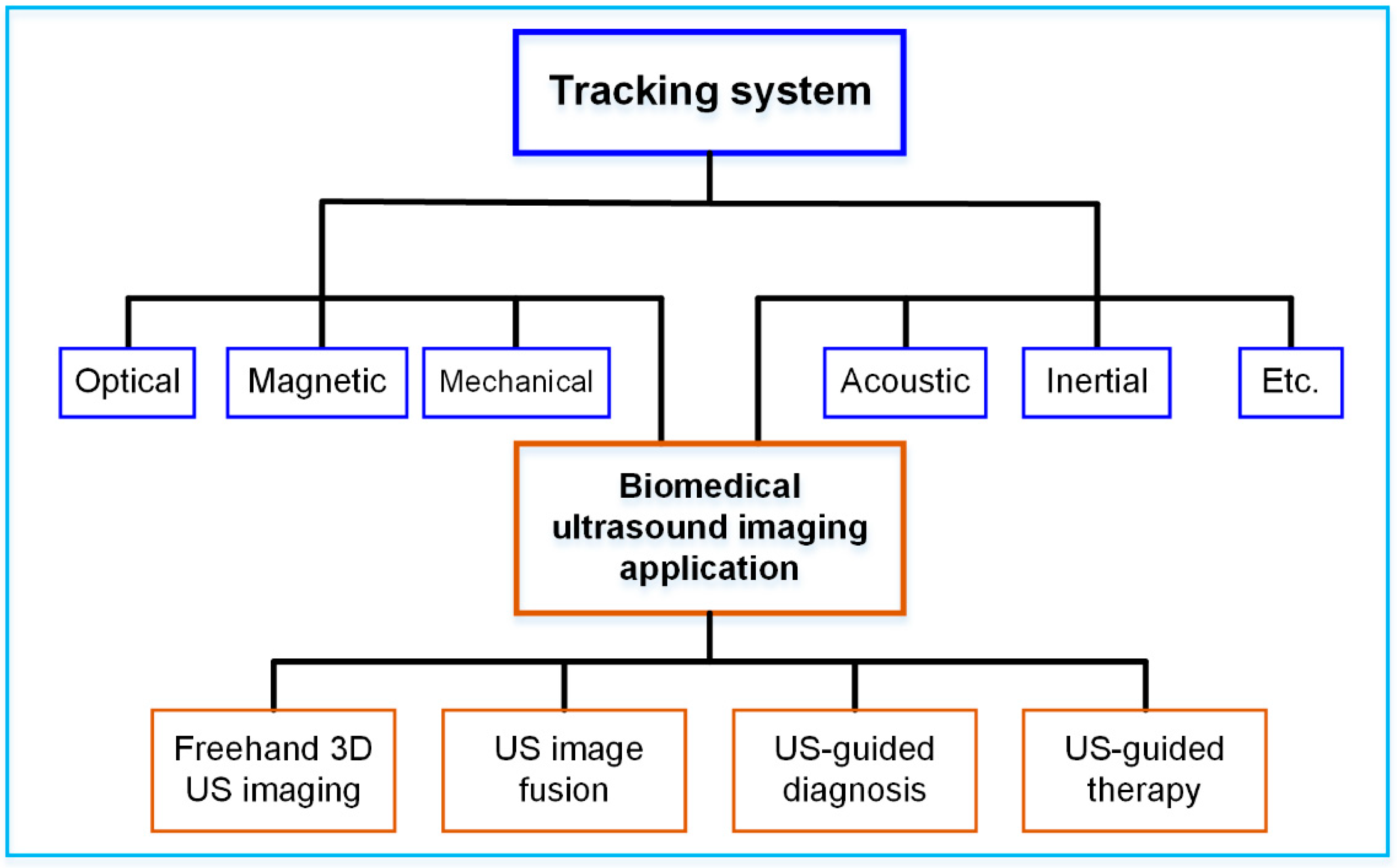
:1. Introduction
2. Physical Principles of Tracking Technologies
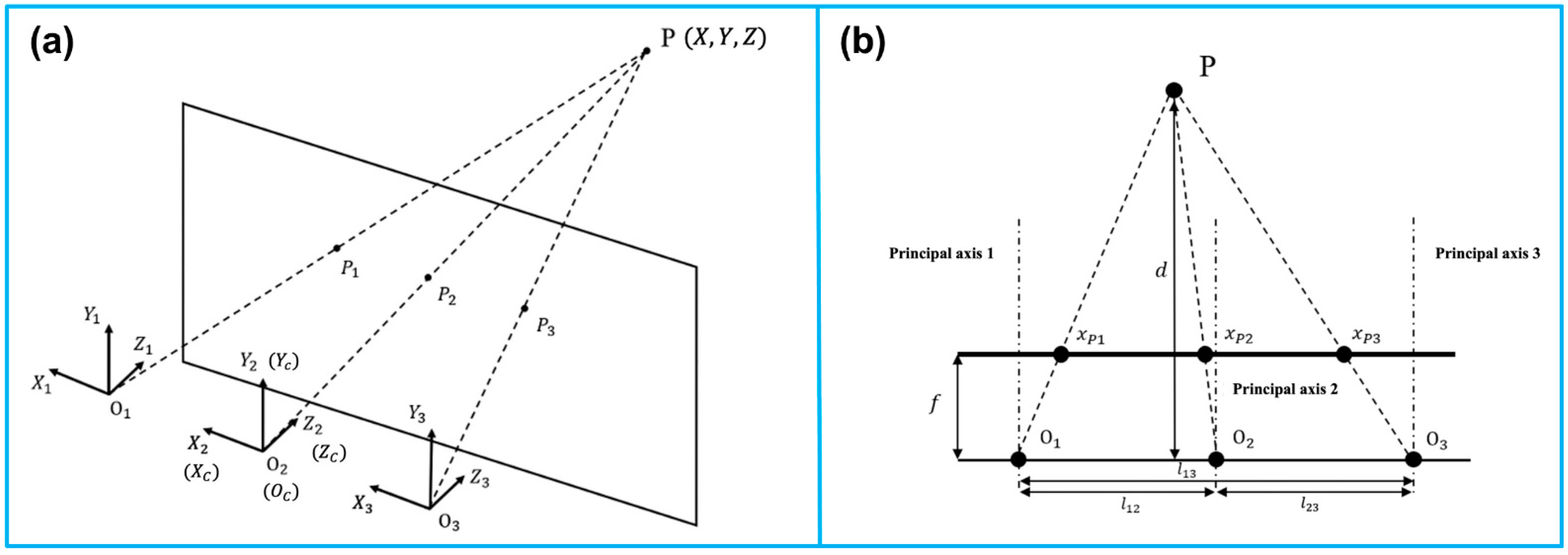
2.1. Optical Tracking
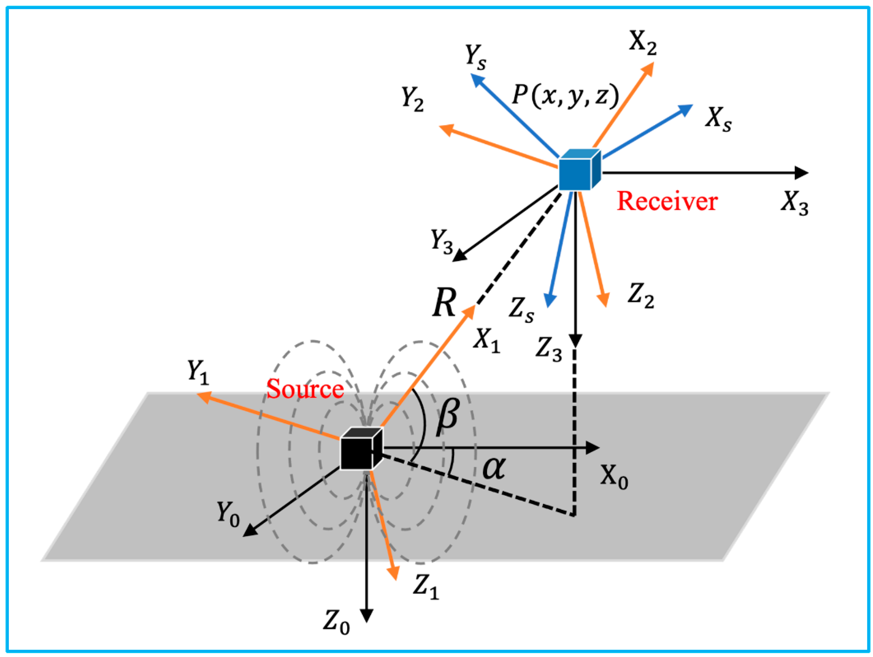
2.2. Electromagnetic Tracking
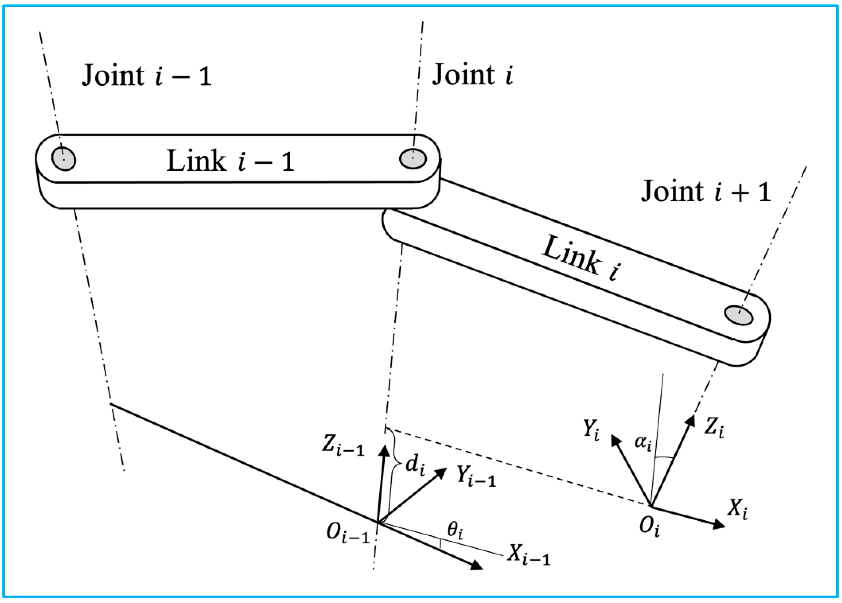
2.3. Mechanical Tracking
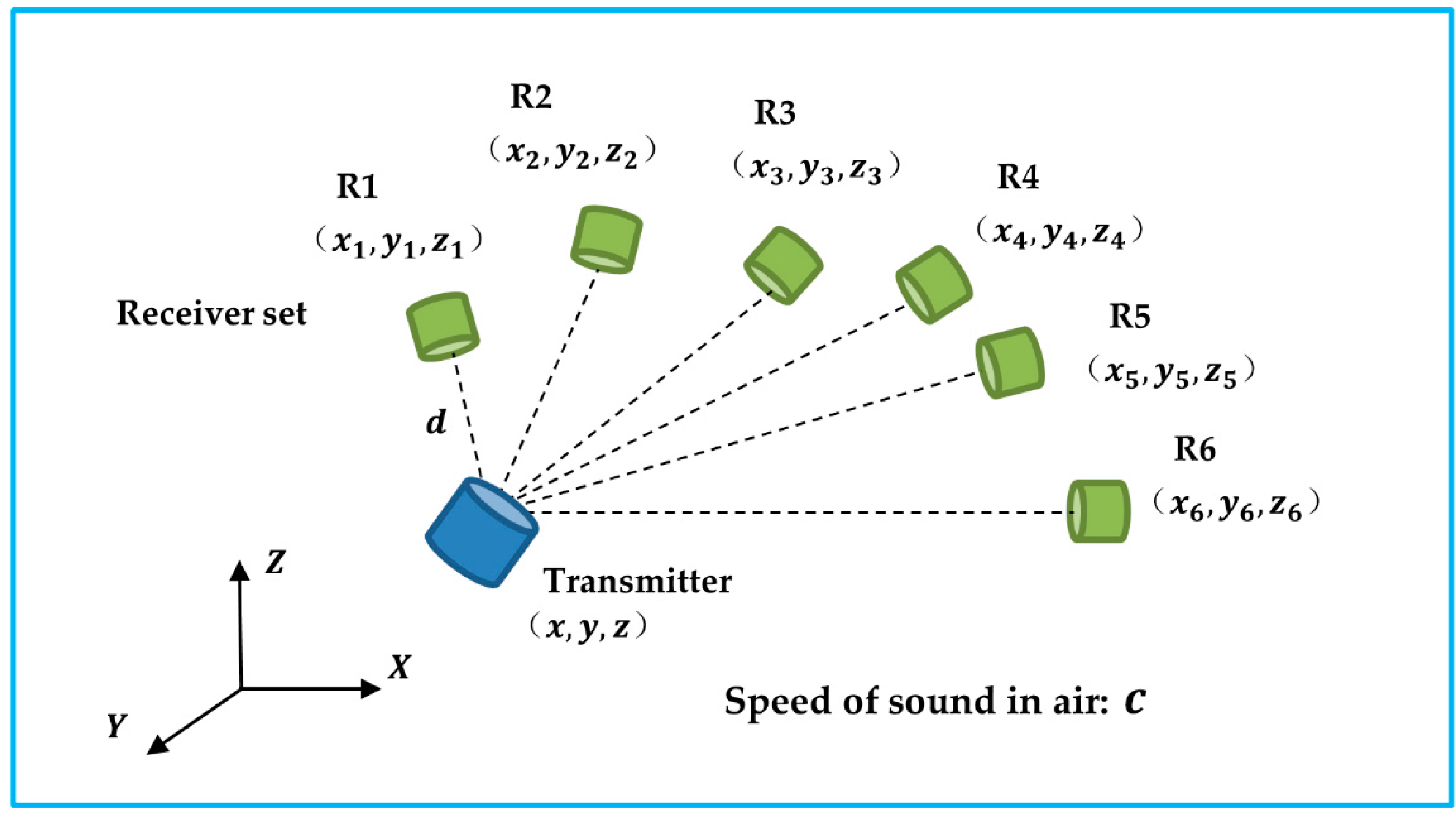
2.4. Acoustic Tracking
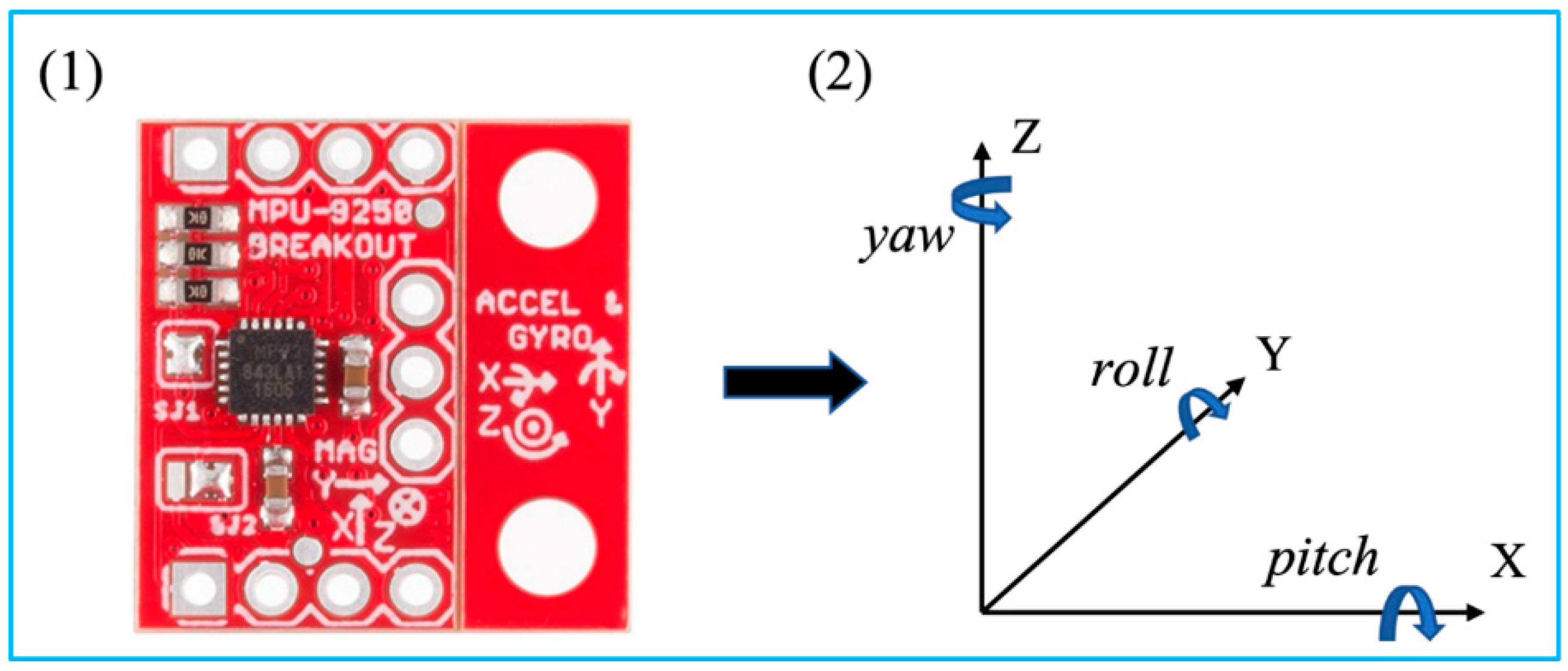
2.5. Inertial Tracking
3. Tracking Systems
3.1. Optical Tracking Systems
3.2. Electromagnetic Tracking Systems
3.3. Mechanical Tracking Systems
3.4. Acoustic Tracking Systems
3.5. Inertial Tracking Systems
4. Biomedical Ultrasound Imaging Applications
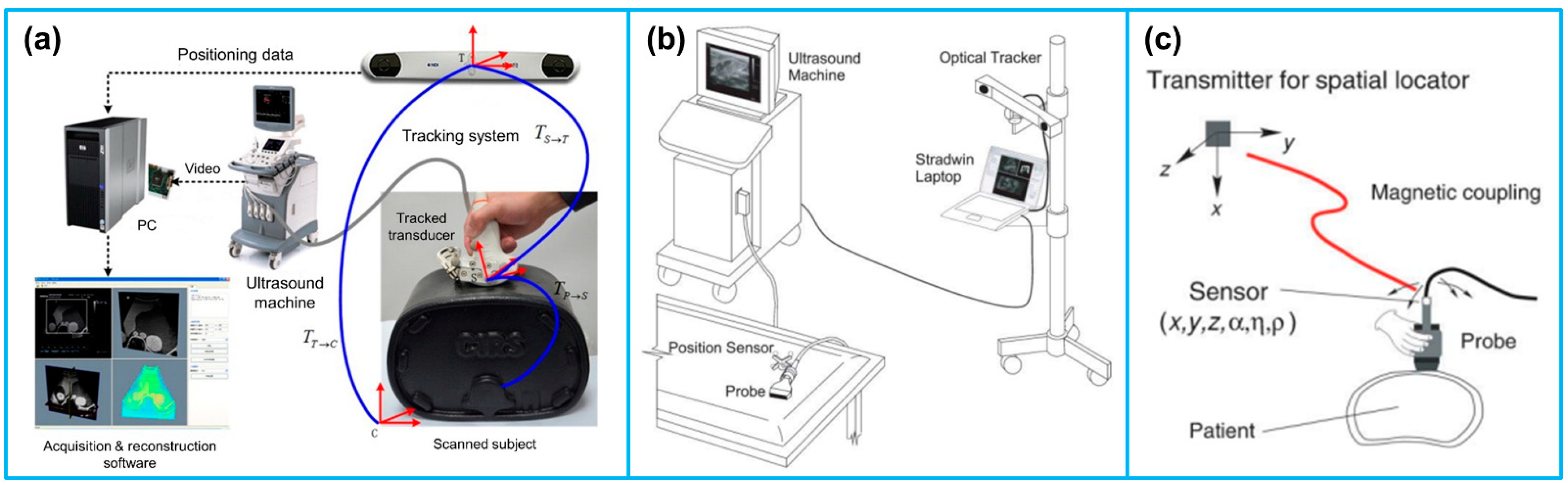
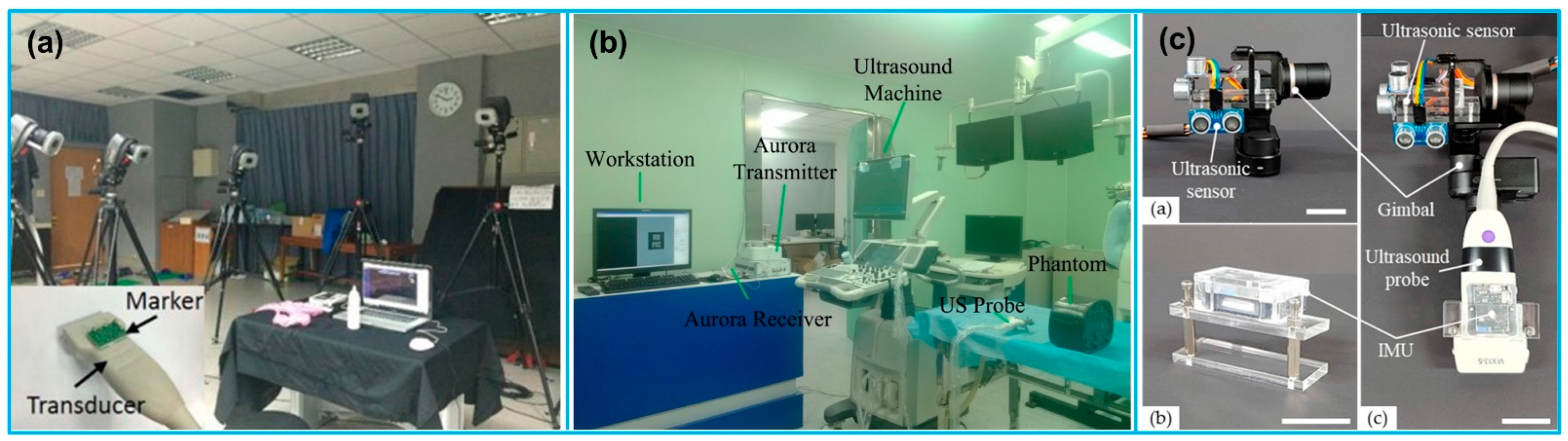
4.1. Freehand 3D Ultrasound Imaging


| Reference | Tracking Principle | Tracking System | Accuracy | Application |
|---|---|---|---|---|
| Chung et al. [116] | Optical tracking | Motion Analysis, Santa Rosa, CA, USA | Spatial: 10 μm Temporal: 0.01 s | Carotid atherosclerotic stenosis detection |
| Pelz et al. [119] | Electromagnetic tracking | Curefab CS system (Curefab Technologies GmbH, Munich, Germany) | None | Internal carotid artery stenosis diagnosis |
| Miller et al. [120] | Optical tracking | VectorVision2 navigation system (BrainLAB, Munich, Germany) | None | Image-guided surgery |
| Mercier et al. [121] | Optical tracking | Polaris (Northern Digital, Waterloo, ON, Canada) | Spatial: 0.49–0.74 mm Temporal: 82 ms | Neuronavigation |
| Chen et al. [122] | Electromagnetic tracking | Aurora (NDI, ON, Canada) | None | Image-guided surgery |
| Wen et al. [115] | Optical tracking | Polaris (Northern Digital, Waterloo, ON, Canada) | None | Image-guided intervention |
| Sun et al. [123] | Optical tracking | OptiTrack V120:Trio (NaturalPoint Inc., Corvallis, OR, USA) | Spatial: <1 mm | Image-guided intervention |
| Worobey et al. [124] | Optical tracking | Vicon Motion Systems; Centennial, Colorado | None | Scapular position |
| Passmore et al. [125] | Optical tracking | Vicon Motion Systems, Oxford, UK | None | Femoral torsion measurement |
| Daoud et al. [117] | Electromagnetic tracking | trakSTAR, NDI, ON, Canada | None | 3D US imaging |
| Chen and Huang [118] | Electromagnetic tracking | MiniBird, Ascension Technology Corp., Burlington, VT, USA | None | Real-time 3D imaging |
| Cai et al. [20] | Optical tracking | OptiTrack V120: Trio (NaturalPoint Inc., Corvallis, OR, USA) | Positional: 0.08–0.69 mm Rotational: 0.33–0.62° | 3D US imaging |
| Herickhoff et al. [17] | Inertial tracking | IMU sensor (iNEMO-M1; STMicroelectronics, Geneva, Switzerland) | None | Low-cost 3D imaging platform |
| Kim et al. [126] | Inertial tracking | Ultrasonic sensor + IMU sensor (HC-SR04, Shenzhen AV, Shenzhen, China) | Spatial: 0.79–1.25 mm | Low-cost 3D imaging platform |
| Lai et al. [127] | Optical tracking | T265, Intel, Santa Clara, CA, USA | Spatial: 2.9 ± 1.8° | Scoliosis assessment |
| Jiang et al. [128] | Electromagnetic tracking | Ascension Technology, Burlington, VT, USA | None | Scoliosis assessment |

4.2. Ultrasound Image Fusion in Multimodality Imaging
4.3. Ultrasound-Guided Diagnosis
4.4. Ultrasound-Guided Therapy
5. Conclusions
6. Future Perspectives
Author Contributions
Funding
Acknowledgments
Conflicts of Interest
Abbreviations
| 2D | Two dimensions |
| 3D | Three dimensions |
| CCD | Charge-coupled device |
| Corp. | Corporation |
| CT | Computed tomography |
| DOF | Degree-of-freedom |
| ECIRS | Endoscopic combined intrarenal surgery |
| FDA | Food and drug administration |
| FOV | Field of view |
| FPS | Frames per second |
| GPU | Graphics processing unit |
| HCC | Hepatocellular carcinoma |
| HDR | High-dose-rate |
| IMU | Inertial measurement unit |
| Inc. | Incorporated |
| LED | Light emitting diode |
| MEMS | Microelectromechanical system |
| MP | Megapixel |
| MRI | Magnetic resonance imaging |
| NDI | Northern Digital Inc. |
| PCNL | Percutaneous nephrolithotomy |
| PET | Positron emission tomography |
| RMS | Root mean square |
| RVS | Real-time virtual sonography |
| TDOA | Time difference of arrival |
| TDOF | Time difference of flight |
| TOA | Time of arrival |
| TOF | Time of flight |
| TRUS | Transrectal ultrasound |
| US | Ultrasound |
| USB | Universal serial bus |
References
- Kothiya, S.V.; Mistree, K.B. A Review on Real Time Object Tracking in Video Sequences. In Proceedings of the Electrical, Electronics, Signals, Communication and Optimization (EESCO), 2015 International Conference on, Visakhapatnam, India, 24–25 January 2015; pp. 1–4. [Google Scholar]
- Octorina Dewi, D.E.; Supriyanto, E.; Lai, K.W. Position Tracking Systems for Ultrasound Imaging: A Survey. In Medical Imaging Technology; Springer: Berlin/Heidelberg, Germany, 2015; pp. 57–89. [Google Scholar]
- Karayiannidis, Y.; Rovithakis, G.; Doulgeri, Z. Force/Position Tracking for a Robotic Manipulator in Compliant Contact with a Surface Using Neuro-Adaptive Control. Automatica 2007, 43, 1281–1288. [Google Scholar] [CrossRef]
- Chang, Y.-C.; Yen, H.-M. Design of a Robust Position Feedback Tracking Controller for Flexible-Joint Robots. IET Control Theory Appl. 2011, 5, 351–363. [Google Scholar] [CrossRef]
- Liu, M.; Yu, J.; Yang, L.; Yao, L.; Zhang, Y. Consecutive Tracking for Ballistic Missile Based on Bearings-Only during Boost Phase. J. Syst. Eng. Electron. 2012, 23, 700–707. [Google Scholar] [CrossRef]
- Kendoul, F. Survey of Advances in Guidance, Navigation, and Control of Unmanned Rotorcraft Systems. J. Field Robot. 2012, 29, 315–378. [Google Scholar] [CrossRef]
- Ren, H.; Rank, D.; Merdes, M.; Stallkamp, J.; Kazanzides, P. Multisensor Data Fusion in an Integrated Tracking System for Endoscopic Surgery. IEEE Trans. Inf. Technol. Biomed. 2011, 16, 106–111. [Google Scholar] [CrossRef] [PubMed]
- Huang, Q.-H.; Yang, Z.; Hu, W.; Jin, L.-W.; Wei, G.; Li, X. Linear Tracking for 3-D Medical Ultrasound Imaging. IEEE Trans. Cybern. 2013, 43, 1747–1754. [Google Scholar] [CrossRef] [PubMed]
- Leser, R.; Baca, A.; Ogris, G. Local Positioning Systems in (Game) Sports. Sensors 2011, 11, 9778–9797. [Google Scholar] [CrossRef] [Green Version]
- Hedley, M.; Zhang, J. Accurate Wireless Localization in Sports. Computer 2012, 45, 64–70. [Google Scholar] [CrossRef]
- Mozaffari, M.H.; Lee, W.-S. Freehand 3-D Ultrasound Imaging: A Systematic Review. Ultrasound Med. Biol. 2017, 43, 2099–2124. [Google Scholar] [CrossRef] [Green Version]
- Cleary, K.; Peters, T.M. Image-Guided Interventions: Technology Review and Clinical Applications. Annu. Rev. Biomed. Eng. 2010, 12, 119–142. [Google Scholar] [CrossRef]
- Lindseth, F.; Langø, T.; Selbekk, T.; Hansen, R.; Reinertsen, I.; Askeland, C.; Solheim, O.; Unsgård, G.; Mårvik, R.; Hernes, T.A.N. Ultrasound-Based Guidance and Therapy. In Advancements and Breakthroughs in Ultrasound Imaging; IntechOpen: London, UK, 2013. [Google Scholar]
- Zhou, H.; Hu, H. Human Motion Tracking for Rehabilitation—A Survey. Biomed. Signal Process. Control 2008, 3, 1–18. [Google Scholar] [CrossRef]
- Moran, C.M.; Thomson, A.J.W. Preclinical Ultrasound Imaging—A Review of Techniques and Imaging Applications. Front. Phys. 2020, 8, 124. [Google Scholar] [CrossRef]
- Fenster, A.; Downey, D.B.; Cardinal, H.N. Three-Dimensional Ultrasound Imaging. Phys. Med. Biol. 2001, 46, R67. [Google Scholar] [CrossRef]
- Herickhoff, C.D.; Morgan, M.R.; Broder, J.S.; Dahl, J.J. Low-Cost Volumetric Ultrasound by Augmentation of 2D Systems: Design and Prototype. Ultrason. Imaging 2018, 40, 35–48. [Google Scholar] [CrossRef] [PubMed]
- Schlegel, M. Predicting the Accuracy of Optical Tracking Systems; Technical University of Munich: München, Germany, 2006. [Google Scholar]
- Abdelhamid, M. Extracting Depth Information from Stereo Vision System: Using a Correlation and a Feature Based Methods. Master’s Thesis, Clemson University, Clemson, SC, USA, 2011. [Google Scholar]
- Cai, Q.; Peng, C.; Lu, J.; Prieto, J.C.; Rosenbaum, A.J.; Stringer, J.S.A.; Jiang, X. Performance Enhanced Ultrasound Probe Tracking with a Hemispherical Marker Rigid Body. IEEE Trans. Ultrason. Ferroelectr. Freq. Control 2021, 68, 2155–2163. [Google Scholar] [CrossRef] [PubMed]
- Zhigang, Y.; Kui, Y. An Improved 6DOF Electromagnetic Tracking Algorithm with Anisotropic System Parameters. In International Conference on Technologies for E-Learning and Digital Entertainment; Springer: Berlin/Heidelberg, Germany, 2006; pp. 1141–1150. [Google Scholar]
- Zhang, Z.; Liu, G. The Design and Analysis of Electromagnetic Tracking System. J. Electromagn. Anal. Appl. 2013, 5, 85–89. [Google Scholar] [CrossRef] [Green Version]
- Craig, J.J. Introduction to Robotics: Mechanics and Control, 4th ed.; Pearson Education: New York, NY, USA, 2018. [Google Scholar]
- Gueuning, F.; Varlan, M.; Eugene, C.; Dupuis, P. Accurate Distance Measurement by an Autonomous Ultrasonic System Combining Time-of-Flight and Phase-Shift Methods. In Proceedings of the Quality Measurement: The Indispensable Bridge between Theory and Reality, Brussels, Belgium, 4–6 June 1996; Volume 1, pp. 399–404. [Google Scholar]
- Mahajan, A.; Walworth, M. 3D Position Sensing Using the Differences in the Time-of-Flights from a Wave Source to Various Receivers. IEEE Trans. Robot. Autom. 2001, 17, 91–94. [Google Scholar] [CrossRef]
- Ray, P.K.; Mahajan, A. A Genetic Algorithm-Based Approach to Calculate the Optimal Configuration of Ultrasonic Sensors in a 3D Position Estimation System. Rob. Auton. Syst. 2002, 41, 165–177. [Google Scholar] [CrossRef]
- Cai, Q.; Hu, J.; Chen, M.; Prieto, J.; Rosenbaum, A.J.; Stringer, J.S.A.; Jiang, X. Inertial Measurement Unit Assisted Ultrasonic Tracking System for Ultrasound Probe Localization. IEEE Trans. Ultrason. Ferroelectr. Freq. Control 2022. [Google Scholar] [CrossRef]
- Filippeschi, A.; Schmitz, N.; Miezal, M.; Bleser, G.; Ruffaldi, E.; Stricker, D. Survey of Motion Tracking Methods Based on Inertial Sensors: A Focus on Upper Limb Human Motion. Sensors 2017, 17, 1257. [Google Scholar] [CrossRef]
- Patonis, P.; Patias, P.; Tziavos, I.N.; Rossikopoulos, D.; Margaritis, K.G. A Fusion Method for Combining Low-Cost IMU/Magnetometer Outputs for Use in Applications on Mobile Devices. Sensors 2018, 18, 2616. [Google Scholar] [CrossRef] [PubMed] [Green Version]
- Arqus. Available online: https://www.qualisys.com/cameras/arqus/#!%23tech-specs (accessed on 27 September 2022).
- Polaris Vega® ST. Available online: https://www.ndigital.com/optical-measurement-technology/polaris-vega/polaris-vega-st/ (accessed on 27 September 2022).
- Polaris Vega® VT. Available online: https://www.ndigital.com/optical-measurement-technology/polaris-vega/polaris-vega-vt/ (accessed on 27 September 2022).
- Polaris Vega® XT. Available online: https://www.ndigital.com/optical-measurement-technology/polaris-vega/polaris-vega-xt/ (accessed on 27 September 2022).
- Polaris Vicra®. Available online: https://www.ndigital.com/optical-measurement-technology/polaris-vicra/ (accessed on 27 September 2022).
- ClaroNav MicronTracker Specification. Available online: https://www.claronav.com/microntracker/microntracker-specifications/ (accessed on 27 September 2022).
- Smart DX. Available online: https://www.btsbioengineering.com/products/smart-dx-motion-capture/ (accessed on 27 September 2022).
- PrimeX 41. Available online: https://optitrack.com/cameras/primex-41/specs.html (accessed on 27 September 2022).
- PrimeX 22. Available online: https://optitrack.com/cameras/primex-22/specs.html (accessed on 27 September 2022).
- PrimeX 13. Available online: https://optitrack.com/cameras/primex-13/specs.html (accessed on 27 September 2022).
- PrimeX 13W. Available online: https://optitrack.com/cameras/primex-13w/specs.html (accessed on 27 September 2022).
- SlimX 13. Available online: https://optitrack.com/cameras/slimx-13/specs.html (accessed on 27 September 2022).
- V120:Trio. Available online: https://optitrack.com/cameras/v120-trio/specs.html (accessed on 27 September 2022).
- V120:Duo. Available online: https://optitrack.com/cameras/v120-duo/specs.html (accessed on 27 September 2022).
- Flex 13. Available online: https://optitrack.com/cameras/flex-13/specs.html (accessed on 27 September 2022).
- Flex 3. Available online: https://optitrack.com/cameras/flex-3/specs.html (accessed on 27 September 2022).
- Slim 3U. Available online: https://optitrack.com/cameras/slim-3u/specs.html (accessed on 27 September 2022).
- TrackIR 4. vs. TrackIR 5. Available online: https://www.trackir.com/trackir5/ (accessed on 27 September 2022).
- Miqus. Available online: https://www.qualisys.com/cameras/miqus/#tech-specs (accessed on 27 September 2022).
- Miqus Hybrid. Available online: https://www.qualisys.com/cameras/miqus-hybrid/#tech-specs (accessed on 27 September 2022).
- 5+, 6+ and 7+ Series. Available online: https://www.qualisys.com/cameras/5-6-7/#tech-specs (accessed on 27 September 2022).
- Valkyrie. Available online: https://www.vicon.com/hardware/cameras/valkyrie/ (accessed on 27 September 2022).
- Vantage+. Available online: https://www.vicon.com/hardware/cameras/vantage/ (accessed on 27 September 2022).
- Vero. Available online: https://www.vicon.com/hardware/cameras/vero/ (accessed on 27 September 2022).
- Vue. Available online: https://www.vicon.com/hardware/cameras/vue/ (accessed on 27 September 2022).
- Viper. Available online: https://www.vicon.com/hardware/cameras/viper/ (accessed on 27 September 2022).
- ViperX. Available online: https://www.vicon.com/hardware/cameras/viper-x/ (accessed on 27 September 2022).
- FusionTrack 500. Available online: https://www.atracsys-measurement.com/fusiontrack-500/ (accessed on 27 September 2022).
- FusionTrack 250. Available online: https://www.atracsys-measurement.com/fusiontrack-250/ (accessed on 27 September 2022).
- SpryTrack 180. Available online: https://www.atracsys-measurement.com/sprytrack-180/ (accessed on 27 September 2022).
- SpryTrack 300. Available online: https://www.atracsys-measurement.com/sprytrack-300/ (accessed on 27 September 2022).
- Kestrel 4200. Available online: https://motionanalysis.com/blog/cameras/kestrel-4200/ (accessed on 27 September 2022).
- Kestrel 2200. Available online: https://motionanalysis.com/blog/cameras/kestrel-2200/ (accessed on 27 September 2022).
- Kestrel 1300. Available online: https://motionanalysis.com/blog/cameras/kestrel-130/ (accessed on 27 September 2022).
- Kestrel 300. Available online: https://motionanalysis.com/blog/cameras/kestrel-300/ (accessed on 27 September 2022).
- EDDO Biomechanic. Available online: https://www.stt-systems.com/motion-analysis/3d-optical-motion-capture/eddo/ (accessed on 27 September 2022).
- ARTTRACK6/M. Available online: https://ar-tracking.com/en/product-program/arttrack6m (accessed on 27 September 2022).
- ARTTRACK5. Available online: https://ar-tracking.com/en/product-program/arttrack5 (accessed on 27 September 2022).
- SMARTTRACK3 & SMARTTRACK3/M. Available online: https://ar-tracking.com/en/product-program/smarttrack3 (accessed on 27 September 2022).
- Micro Sensor 1.8. Available online: https://polhemus.com/micro-sensors/ (accessed on 27 September 2022).
- Aurora. Available online: https://www.ndigital.com/electromagnetic-tracking-technology/aurora/ (accessed on 27 September 2022).
- 3D Guidance. Available online: https://www.ndigital.com/electromagnetic-tracking-technology/3d-guidance/ (accessed on 27 September 2022).
- Viper. Available online: https://polhemus.com/viper (accessed on 27 September 2022).
- Fastrak. Available online: https://polhemus.com/motion-tracking/all-trackers/fastrak (accessed on 27 September 2022).
- Patriot. Available online: https://polhemus.com/motion-tracking/all-trackers/patriot (accessed on 27 September 2022).
- Patriot Wireless. Available online: https://polhemus.com/motion-tracking/all-trackers/patriot-wireless (accessed on 27 September 2022).
- Liberty. Available online: https://polhemus.com/motion-tracking/all-trackers/liberty (accessed on 27 September 2022).
- Liberty Latus. Available online: https://polhemus.com/motion-tracking/all-trackers/liberty-latus (accessed on 27 September 2022).
- G4. Available online: https://polhemus.com/motion-tracking/all-trackers/g4 (accessed on 27 September 2022).
- Gypsy 7. Available online: https://metamotion.com/gypsy/gypsy-motion-capture-system.htm (accessed on 27 September 2022).
- Forkbeard. Available online: https://www.sonitor.com/forkbeard (accessed on 27 September 2022).
- Xsens DOT. Available online: https://www.xsens.com/xsens-dot (accessed on 27 September 2022).
- MTw Awinda. Available online: https://www.xsens.com/products/mtw-awinda (accessed on 27 September 2022).
- MTi 1-Series. Available online: https://mtidocs.xsens.com/sensor-specifications$mti-1-series-performance-specifications (accessed on 27 September 2022).
- MTi 10/100-Series. Available online: https://mtidocs.xsens.com/output-specifications$orientation-performance-specification (accessed on 27 September 2022).
- MTi 600-Series. Available online: https://mtidocs.xsens.com/sensor-specifications-2$mti-600-series-performance-specifications-nbsp (accessed on 27 September 2022).
- Inertial Motion Capture. Available online: https://www.stt-systems.com/motion-analysis/inertial-motion-capture/ (accessed on 27 September 2022).
- VN-100. Available online: https://www.vectornav.com/products/detail/vn-100 (accessed on 27 September 2022).
- VN-110. Available online: https://www.vectornav.com/products/detail/vn-110 (accessed on 27 September 2022).
- VN-200. Available online: https://www.vectornav.com/products/detail/vn-200 (accessed on 27 September 2022).
- VN-210. Available online: https://www.vectornav.com/products/detail/vn-210 (accessed on 27 September 2022).
- VN-300. Available online: https://www.vectornav.com/products/detail/vn-300 (accessed on 27 September 2022).
- VN-310. Available online: https://www.vectornav.com/products/detail/vn-310 (accessed on 27 September 2022).
- Motus. Available online: https://www.advancednavigation.com/imu-ahrs/mems-imu/motus/ (accessed on 27 September 2022).
- Orientus. Available online: https://www.advancednavigation.com/imu-ahrs/mems-imu/orientus/ (accessed on 27 September 2022).
- BOREAS D90. Available online: https://www.advancednavigation.com/inertial-navigation-systems/fog-gnss-ins/boreas/ (accessed on 27 September 2022).
- Spatial FOG Dual. Available online: https://www.advancednavigation.com/inertial-navigation-systems/fog-gnss-ins/spatial-fog-dual/ (accessed on 27 September 2022).
- Certus Evo. Available online: https://www.advancednavigation.com/inertial-navigation-systems/mems-gnss-ins/certus-evo/ (accessed on 27 September 2022).
- Certus. Available online: https://www.advancednavigation.com/inertial-navigation-systems/mems-gnss-ins/certus/ (accessed on 27 September 2022).
- Spatial. Available online: https://www.advancednavigation.com/inertial-navigation-systems/mems-gnss-ins/spatial/ (accessed on 27 September 2022).
- GNSS Compass. Available online: https://www.advancednavigation.com/inertial-navigation-systems/satellite-compass/gnss-compass/ (accessed on 27 September 2022).
- Kernel-100. Available online: https://inertiallabs.com/wp-content/uploads/2021/12/IMU-Kernel_Datasheet.rev_.2.9_December_2021.pdf (accessed on 27 September 2022).
- Kernel-110, 120. Available online: https://inertiallabs.com/wp-content/uploads/2022/09/IMU-Kernel-110-120_Datasheet.rev1_.7_September20_2022.pdf (accessed on 27 September 2022).
- Kernel-210, 220. Available online: https://inertiallabs.com/wp-content/uploads/2022/09/IMU-Kernel-210-220_Datasheet.rev1_.6_Sept20_2022.pdf (accessed on 27 September 2022).
- IMU-P. Available online: https://inertiallabs.com/wp-content/uploads/2022/09/IMU-P_Datasheet.rev4_.1_Sept20_2022.pdf (accessed on 27 September 2022).
- Peng, C.; Chen, M.; Spicer, J.B.; Jiang, X. Acoustics at the Nanoscale (Nanoacoustics): A Comprehensive Literature Review. Part II: Nanoacoustics for Biomedical Imaging and Therapy. Sens. Actuators A Phys. 2021, 332, 112925. [Google Scholar] [CrossRef] [PubMed]
- Rajaraman, P.; Simpson, J.; Neta, G.; de Gonzalez, A.B.; Ansell, P.; Linet, M.S.; Ron, E.; Roman, E. Early Life Exposure to Diagnostic Radiation and Ultrasound Scans and Risk of Childhood Cancer: Case-Control Study. BMJ 2011, 342, d472. [Google Scholar] [CrossRef] [PubMed] [Green Version]
- Huang, Q.; Zeng, Z. A Review on Real-Time 3D Ultrasound Imaging Technology. Biomed. Res. Int. 2017, 2017, 6027029. [Google Scholar] [CrossRef] [Green Version]
- Morgan, M.R.; Broder, J.S.; Dahl, J.J.; Herickhoff, C.D. Versatile Low-Cost Volumetric 3-D Ultrasound Platform for Existing Clinical 2-D Systems. IEEE Trans. Med. Imaging 2018, 37, 2248–2256. [Google Scholar] [CrossRef]
- Prager, R.W.; Ijaz, U.Z.; Gee, A.H.; Treece, G.M. Three-Dimensional Ultrasound Imaging. Proc. Inst. Mech. Eng. Part H J. Eng. Med. 2010, 224, 193–223. [Google Scholar] [CrossRef]
- Fenster, A.; Parraga, G.; Bax, J. Three-Dimensional Ultrasound Scanning. Interface Focus 2011, 1, 503–519. [Google Scholar] [CrossRef] [Green Version]
- Yen, J.T.; Steinberg, J.P.; Smith, S.W. Sparse 2-D Array Design for Real Time Rectilinear Volumetric Imaging. IEEE Trans. Ultrason. Ferroelectr. Freq. Control 2000, 47, 93–110. [Google Scholar] [CrossRef] [Green Version]
- Yen, J.T.; Smith, S.W. Real-Time Rectilinear 3-D Ultrasound Using Receive Mode Multiplexing. ieee Trans. Ultrason. Ferroelectr. Freq. Control 2004, 51, 216–226. [Google Scholar] [CrossRef]
- Turnbull, D.H.; Foster, F.S. Fabrication and Characterization of Transducer Elements in Two-Dimensional Arrays for Medical Ultrasound Imaging. IEEE Trans. Ultrason. Ferroelectr. Freq. Control 1992, 39, 464–475. [Google Scholar] [CrossRef]
- Gee, A.; Prager, R.; Treece, G.; Berman, L. Engineering a Freehand 3D Ultrasound System. Pattern Recognit. Lett. 2003, 24, 757–777. [Google Scholar] [CrossRef]
- Wen, T.; Yang, F.; Gu, J.; Wang, L. A Novel Bayesian-Based Nonlocal Reconstruction Method for Freehand 3D Ultrasound Imaging. Neurocomputing 2015, 168, 104–118. [Google Scholar] [CrossRef]
- Chung, S.-W.; Shih, C.-C.; Huang, C.-C. Freehand Three-Dimensional Ultrasound Imaging of Carotid Artery Using Motion Tracking Technology. Ultrasonics 2017, 74, 11–20. [Google Scholar] [CrossRef] [PubMed]
- Daoud, M.I.; Alshalalfah, A.-L.; Awwad, F.; Al-Najar, M. Freehand 3D Ultrasound Imaging System Using Electromagnetic Tracking. In Proceedings of the 2015 International Conference on Open Source Software Computing (OSSCOM), Amman, Jordan, 10–13 September 2015; pp. 1–5. [Google Scholar]
- Chen, Z.; Huang, Q. Real-Time Freehand 3D Ultrasound Imaging. Comput. Methods Biomech. Biomed. Eng. Imaging Vis. 2018, 6, 74–83. [Google Scholar] [CrossRef]
- Pelz, J.O.; Weinreich, A.; Karlas, T.; Saur, D. Evaluation of Freehand B-Mode and Power-Mode 3D Ultrasound for Visualisation and Grading of Internal Carotid Artery Stenosis. PLoS ONE 2017, 12, e0167500. [Google Scholar] [CrossRef] [PubMed] [Green Version]
- Miller, D.; Lippert, C.; Vollmer, F.; Bozinov, O.; Benes, L.; Schulte, D.M.; Sure, U. Comparison of Different Reconstruction Algorithms for Three-dimensional Ultrasound Imaging in a Neurosurgical Setting. Int. J. Med. Robot. Comput. Assist. Surg. 2012, 8, 348–359. [Google Scholar] [CrossRef] [Green Version]
- Mercier, L.; Del Maestro, R.F.; Petrecca, K.; Kochanowska, A.; Drouin, S.; Yan, C.X.B.; Janke, A.L.; Chen, S.J.-S.; Collins, D.L. New Prototype Neuronavigation System Based on Preoperative Imaging and Intraoperative Freehand Ultrasound: System Description and Validation. Int. J. Comput. Assist. Radiol. Surg. 2011, 6, 507–522. [Google Scholar] [CrossRef]
- Chen, X.; Wen, T.; Li, X.; Qin, W.; Lan, D.; Pan, W.; Gu, J. Reconstruction of Freehand 3D Ultrasound Based on Kernel Regression. Biomed. Eng. Online 2014, 13, 1–15. [Google Scholar] [CrossRef] [Green Version]
- Sun, S.-Y.; Gilbertson, M.; Anthony, B.W. Probe Localization for Freehand 3D Ultrasound by Tracking Skin Features. In Medical Image Computing and Computer-Assisted Intervention—MICCAI 2014; Springer: Berlin/Heidelberg, Germany, 2014; pp. 365–372. [Google Scholar]
- Worobey, L.A.; Udofa, I.A.; Lin, Y.-S.; Koontz, A.M.; Farrokhi, S.S.; Boninger, M.L. Reliability of Freehand Three-Dimensional Ultrasound to Measure Scapular Rotations. J. Rehabil. Res. Dev. 2014, 51, 985–994. [Google Scholar] [CrossRef]
- Passmore, E.; Pandy, M.G.; Graham, H.K.; Sangeux, M. Measuring Femoral Torsion in Vivo Using Freehand 3-D Ultrasound Imaging. Ultrasound Med. Biol. 2016, 42, 619–623. [Google Scholar] [CrossRef]
- Kim, T.; Kang, D.-H.; Shim, S.; Im, M.; Seo, B.K.; Kim, H.; Lee, B.C. Versatile Low-Cost Volumetric 3D Ultrasound Imaging Using Gimbal-Assisted Distance Sensors and an Inertial Measurement Unit. Sensors 2020, 20, 6613. [Google Scholar] [CrossRef] [PubMed]
- Lai, K.K.-L.; Lee, T.T.-Y.; Lee, M.K.-S.; Hui, J.C.-H.; Zheng, Y.-P. Validation of Scolioscan Air-Portable Radiation-Free Three-Dimensional Ultrasound Imaging Assessment System for Scoliosis. Sensors 2021, 21, 2858. [Google Scholar] [CrossRef] [PubMed]
- Jiang, W.; Chen, X.; Yu, C. A Real-time Freehand 3D Ultrasound Imaging Method for Scoliosis Assessment. J. Appl. Clin. Med. Phys. 2022, 23, e13709. [Google Scholar] [CrossRef] [PubMed]
- Ewertsen, C.; Săftoiu, A.; Gruionu, L.G.; Karstrup, S.; Nielsen, M.B. Real-Time Image Fusion Involving Diagnostic Ultrasound. Am. J. Roentgenol. 2013, 200, W249–W255. [Google Scholar] [CrossRef] [PubMed]
- Li, X.; Zhou, F.; Tan, H.; Zhang, W.; Zhao, C. Multimodal Medical Image Fusion Based on Joint Bilateral Filter and Local Gradient Energy. Inf. Sci. 2021, 569, 302–325. [Google Scholar] [CrossRef]
- Klibanov, A.L.; Hossack, J.A. Ultrasound in Radiology: From Anatomic, Functional, Molecular Imaging to Drug Delivery and Image-Guided Therapy. Investig. Radiol. 2015, 50, 657. [Google Scholar] [CrossRef] [Green Version]
- Baad, M.; Lu, Z.F.; Reiser, I.; Paushter, D. Clinical Significance of US Artifacts. Radiographics 2017, 37, 1408–1423. [Google Scholar] [CrossRef] [Green Version]
- European Society of Radiology (ESR) communications@ myesr. org D’Onofrio Mirko Beleù Alessandro Gaitini Diana Corréas Jean-Michel Brady Adrian Clevert Dirk. Abdominal Applications of Ultrasound Fusion Imaging Technique: Liver, Kidney, and Pancreas. Insights Imaging 2019, 10, 6. [Google Scholar] [CrossRef] [Green Version]
- Chien, C.P.Y.; Lee, K.H.; Lau, V. Real-Time Ultrasound Fusion Imaging–Guided Interventions: A Review. Hong Kong J. Radiol. 2021, 24, 116. [Google Scholar] [CrossRef]
- Natarajan, S.; Marks, L.S.; Margolis, D.J.A.; Huang, J.; Macairan, M.L.; Lieu, P.; Fenster, A. Clinical Application of a 3D Ultrasound-Guided Prostate Biopsy System. In Urologic Oncology: Seminars and Original Investigations; Elsevier: Amsterdam, The Netherlands, 2011; Volume 29, pp. 334–342. [Google Scholar]
- Krücker, J.; Xu, S.; Venkatesan, A.; Locklin, J.K.; Amalou, H.; Glossop, N.; Wood, B.J. Clinical Utility of Real-Time Fusion Guidance for Biopsy and Ablation. J. Vasc. Interv. Radiol. 2011, 22, 515–524. [Google Scholar] [CrossRef]
- Appelbaum, L.; Sosna, J.; Nissenbaum, Y.; Benshtein, A.; Goldberg, S.N. Electromagnetic Navigation System for CT-Guided Biopsy of Small Lesions. Am. J. Roentgenol. 2011, 196, 1194–1200. [Google Scholar] [CrossRef] [PubMed]
- Venkatesan, A.M.; Kadoury, S.; Abi-Jaoudeh, N.; Levy, E.B.; Maass-Moreno, R.; Krücker, J.; Dalal, S.; Xu, S.; Glossop, N.; Wood, B.J. Real-Time FDG PET Guidance during Biopsies and Radiofrequency Ablation Using Multimodality Fusion with Electromagnetic Navigation. Radiology 2011, 260, 848–856. [Google Scholar] [CrossRef] [PubMed]
- Lee, M.W. Fusion Imaging of Real-Time Ultrasonography with CT or MRI for Hepatic Intervention. Ultrasonography 2014, 33, 227. [Google Scholar] [CrossRef] [PubMed]
- Sumi, H.; Itoh, A.; Kawashima, H.; Ohno, E.; Itoh, Y.; Nakamura, Y.; Hiramatsu, T.; Sugimoto, H.; Hayashi, D.; Kuwahara, T. Preliminary Study on Evaluation of the Pancreatic Tail Observable Limit of Transabdominal Ultrasonography Using a Position Sensor and CT-Fusion Image. Eur. J. Radiol. 2014, 83, 1324–1331. [Google Scholar] [CrossRef] [PubMed]
- Lee, K.-H.; Lau, V.; Gao, Y.; Li, Y.-L.; Fang, B.X.; Lee, R.; Lam, W.W.-M. Ultrasound-MRI Fusion for Targeted Biopsy of Myopathies. AJR Am. J. Roentgenol. 2019, 212, 1126–1128. [Google Scholar] [CrossRef] [PubMed]
- Burke, C.J.; Bencardino, J.; Adler, R. The Potential Use of Ultrasound-Magnetic Resonance Imaging Fusion Applications in Musculoskeletal Intervention. J. Ultrasound Med. 2017, 36, 217–224. [Google Scholar] [CrossRef] [Green Version]
- Klauser, A.S.; De Zordo, T.; Feuchtner, G.M.; Djedovic, G.; Weiler, R.B.; Faschingbauer, R.; Schirmer, M.; Moriggl, B. Fusion of Real-Time US with CT Images to Guide Sacroiliac Joint Injection in Vitro and in Vivo. Radiology 2010, 256, 547–553. [Google Scholar] [CrossRef] [Green Version]
- Sonn, G.A.; Margolis, D.J.; Marks, L.S. Target Detection: Magnetic Resonance Imaging-Ultrasound Fusion–Guided Prostate Biopsy. In Urologic Oncology: Seminars and Original Investigations; Elsevier: Amsterdam, The Netherlands, 2014; Volume 32, pp. 903–911. [Google Scholar]
- Costa, D.N.; Pedrosa, I.; Donato, F., Jr.; Roehrborn, C.G.; Rofsky, N.M. MR Imaging–Transrectal US Fusion for Targeted Prostate Biopsies: Implications for Diagnosis and Clinical Management. Radiographics 2015, 35, 696–708. [Google Scholar] [CrossRef]
- Appelbaum, L.; Mahgerefteh, S.Y.; Sosna, J.; Goldberg, S.N. Image-Guided Fusion and Navigation: Applications in Tumor Ablation. Tech. Vasc. Interv. Radiol. 2013, 16, 287–295. [Google Scholar] [CrossRef]
- Marks, L.; Young, S.; Natarajan, S. MRI–Ultrasound Fusion for Guidance of Targeted Prostate Biopsy. Curr. Opin. Urol. 2013, 23, 43. [Google Scholar] [CrossRef]
- Park, H.J.; Lee, M.W.; Lee, M.H.; Hwang, J.; Kang, T.W.; Lim, S.; Rhim, H.; Lim, H.K. Fusion Imaging–Guided Percutaneous Biopsy of Focal Hepatic Lesions with Poor Conspicuity on Conventional Sonography. J. Ultrasound Med. 2013, 32, 1557–1564. [Google Scholar] [CrossRef] [PubMed]
- Lee, M.W.; Rhim, H.; Cha, D.I.; Kim, Y.J.; Lim, H.K. Planning US for Percutaneous Radiofrequency Ablation of Small Hepatocellular Carcinomas (1–3 Cm): Value of Fusion Imaging with Conventional US and CT/MR Images. J. Vasc. Interv. Radiol. 2013, 24, 958–965. [Google Scholar] [CrossRef] [PubMed]
- Song, K.D.; Lee, M.W.; Rhim, H.; Cha, D.I.; Chong, Y.; Lim, H.K. Fusion Imaging–Guided Radiofrequency Ablation for Hepatocellular Carcinomas Not Visible on Conventional Ultrasound. Am. J. Roentgenol. 2013, 201, 1141–1147. [Google Scholar] [CrossRef]
- Helck, A.; D’Anastasi, M.; Notohamiprodjo, M.; Thieme, S.; Sommer, W.; Reiser, M.; Clevert, D.A. Multimodality Imaging Using Ultrasound Image Fusion in Renal Lesions. Clin. Hemorheol. Microcirc. 2012, 50, 79–89. [Google Scholar] [CrossRef] [PubMed]
- Andersson, M.; Hashimi, F.; Lyrdal, D.; Lundstam, S.; Hellström, M. Improved Outcome with Combined US/CT Guidance as Compared to US Guidance in Percutaneous Radiofrequency Ablation of Small Renal Masses. Acta Radiol. 2015, 56, 1519–1526. [Google Scholar] [CrossRef] [PubMed]
- Zhang, H.; Chen, G.; Xiao, L.; Ma, X.; Shi, L.; Wang, T.; Yan, H.; Zou, H.; Chen, Q.; Tang, L. Ultrasonic/CT Image Fusion Guidance Facilitating Percutaneous Catheter Drainage in Treatment of Acute Pancreatitis Complicated with Infected Walled-off Necrosis. Pancreatology 2018, 18, 635–641. [Google Scholar] [CrossRef]
- Rübenthaler, J.; Paprottka, K.J.; Marcon, J.; Reiser, M.; Clevert, D.A. MRI and Contrast Enhanced Ultrasound (CEUS) Image Fusion of Renal Lesions. Clin. Hemorheol. Microcirc. 2016, 64, 457–466. [Google Scholar] [CrossRef]
- Guo, Z.; Shi, H.; Li, W.; Lin, D.; Wang, C.; Liu, C.; Yuan, M.; Wu, X.; Xiong, B.; He, X. Chinese Multidisciplinary Expert Consensus: Guidelines on Percutaneous Transthoracic Needle Biopsy. Thorac. Cancer 2018, 9, 1530–1543. [Google Scholar] [CrossRef]
- Beigi, P.; Salcudean, S.E.; Ng, G.C.; Rohling, R. Enhancement of Needle Visualization and Localization in Ultrasound. Int. J. Comput. Assist. Radiol. Surg. 2021, 16, 169–178. [Google Scholar] [CrossRef]
- Holm, H.H.; Skjoldbye, B. Interventional Ultrasound. Ultrasound Med. Biol. 1996, 22, 773–789. [Google Scholar]
- Stone, J.; Beigi, P.; Rohling, R.; Lessoway, V.; Dube, A.; Gunka, V. Novel 3D Ultrasound System for Midline Single-Operator Epidurals: A Feasibility Study on a Porcine Model. Int. J. Obstet. Anesth. 2017, 31, 51–56. [Google Scholar] [CrossRef] [PubMed]
- Scholten, H.J.; Pourtaherian, A.; Mihajlovic, N.; Korsten, H.H.M.; Bouwman, R.A. Improving Needle Tip Identification during Ultrasound-guided Procedures in Anaesthetic Practice. Anaesthesia 2017, 72, 889–904. [Google Scholar] [CrossRef] [PubMed]
- Boctor, E.M.; Choti, M.A.; Burdette, E.C.; Webster Iii, R.J. Three-dimensional Ultrasound-guided Robotic Needle Placement: An Experimental Evaluation. Int. J. Med. Robot. Comput. Assist. Surg. 2008, 4, 180–191. [Google Scholar] [CrossRef] [PubMed] [Green Version]
- Franz, A.M.; März, K.; Hummel, J.; Birkfellner, W.; Bendl, R.; Delorme, S.; Schlemmer, H.-P.; Meinzer, H.-P.; Maier-Hein, L. Electromagnetic Tracking for US-Guided Interventions: Standardized Assessment of a New Compact Field Generator. Int. J. Comput. Assist. Radiol. Surg. 2012, 7, 813–818. [Google Scholar] [CrossRef] [PubMed]
- Xu, H.-X.; Lu, M.-D.; Liu, L.-N.; Guo, L.-H. Magnetic Navigation in Ultrasound-Guided Interventional Radiology Procedures. Clin. Radiol. 2012, 67, 447–454. [Google Scholar] [CrossRef]
- Hakime, A.; Deschamps, F.; De Carvalho, E.G.M.; Barah, A.; Auperin, A.; De Baere, T. Electromagnetic-Tracked Biopsy under Ultrasound Guidance: Preliminary Results. Cardiovasc. Intervent. Radiol. 2012, 35, 898–905. [Google Scholar] [CrossRef]
- März, K.; Franz, A.M.; Seitel, A.; Winterstein, A.; Hafezi, M.; Saffari, A.; Bendl, R.; Stieltjes, B.; Meinzer, H.-P.; Mehrabi, A. Interventional Real-Time Ultrasound Imaging with an Integrated Electromagnetic Field Generator. Int. J. Comput. Assist. Radiol. Surg. 2014, 9, 759–768. [Google Scholar] [CrossRef]
- Wang, X.L.; Stolka, P.J.; Boctor, E.; Hager, G.; Choti, M. The Kinect as an Interventional Tracking System. In Medical Imaging 2012: Image-Guided Procedures, Robotic Interventions, and Modeling; SPIE: Washington, DC, USA, 2012; Volume 8316, pp. 276–281. [Google Scholar]
- Stolka, P.J.; Foroughi, P.; Rendina, M.; Weiss, C.R.; Hager, G.D.; Boctor, E.M. Needle Guidance Using Handheld Stereo Vision and Projection for Ultrasound-Based Interventions. In Medical Image Computing and Computer-Assisted Intervention—MICCAI 2014; Springer: Cham, Switzerland, 2014; pp. 684–691. [Google Scholar]
- Najafi, M.; Abolmaesumi, P.; Rohling, R. Single-Camera Closed-Form Real-Time Needle Tracking for Ultrasound-Guided Needle Insertion. Ultrasound Med. Biol. 2015, 41, 2663–2676. [Google Scholar] [CrossRef]
- Daoud, M.I.; Alshalalfah, A.-L.; Mohamed, O.A.; Alazrai, R. A Hybrid Camera-and Ultrasound-Based Approach for Needle Localization and Tracking Using a 3D Motorized Curvilinear Ultrasound Probe. Med. Image Anal. 2018, 50, 145–166. [Google Scholar] [CrossRef]
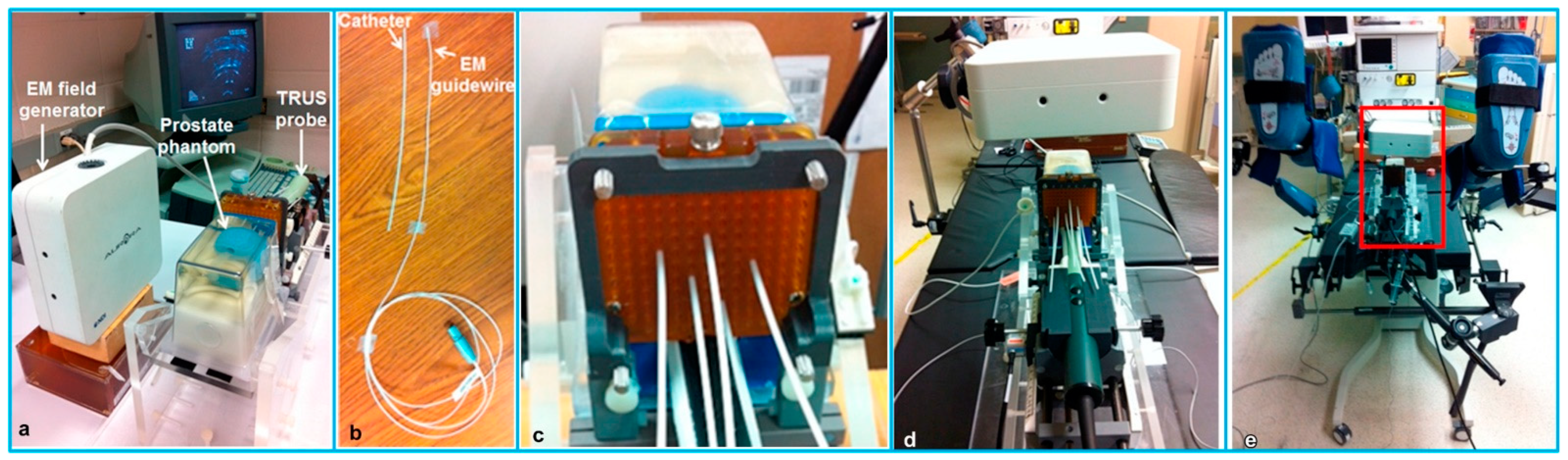
- Ho, H.S.S.; Mohan, P.; Lim, E.D.; Li, D.L.; Yuen, J.S.P.; Ng, W.S.; Lau, W.K.O.; Cheng, C.W.S. Robotic Ultrasound-guided Prostate Intervention Device: System Description and Results from Phantom Studies. Int. J. Med. Robot. Comput. Assist. Surg. 2009, 5, 51–58. [Google Scholar] [CrossRef]
- Orhan, S.O.; Yildirim, M.C.; Bebek, O. Design and Modeling of a Parallel Robot for Ultrasound Guided Percutaneous Needle Interventions. In Proceedings of the IECON 2015—41st Annual Conference of the IEEE Industrial Electronics Society, Yokohama, Japan, 9–12 November 2015; pp. 5002–5007. [Google Scholar]
- Poquet, C.; Mozer, P.; Vitrani, M.-A.; Morel, G. An Endorectal Ultrasound Probe Comanipulator with Hybrid Actuation Combining Brakes and Motors. IEEE/ASME Trans. Mechatron. 2014, 20, 186–196. [Google Scholar] [CrossRef]
- Chen, X.; Bao, N.; Li, J.; Kang, Y. A Review of Surgery Navigation System Based on Ultrasound Guidance. In Proceedings of the 2012 IEEE International Conference on Information and Automation, Shenyang, China, 6–8 June 2012; pp. 882–886. [Google Scholar]
- Stoll, J.; Ren, H.; Dupont, P.E. Passive Markers for Tracking Surgical Instruments in Real-Time 3-D Ultrasound Imaging. IEEE Trans. Med. Imaging 2011, 31, 563–575. [Google Scholar] [CrossRef] [PubMed] [Green Version]
- Li, X.; Long, Q.; Chen, X.; He, D.; He, H. Assessment of the SonixGPS System for Its Application in Real-Time Ultrasonography Navigation-Guided Percutaneous Nephrolithotomy for the Treatment of Complex Kidney Stones. Urolithiasis 2017, 45, 221–227. [Google Scholar] [CrossRef] [PubMed]
- Hamamoto, S.; Unno, R.; Taguchi, K.; Ando, R.; Hamakawa, T.; Naiki, T.; Okada, S.; Inoue, T.; Okada, A.; Kohri, K. A New Navigation System of Renal Puncture for Endoscopic Combined Intrarenal Surgery: Real-Time Virtual Sonography-Guided Renal Access. Urology 2017, 109, 44–50. [Google Scholar] [CrossRef]
- Gomes-Fonseca, J.; Veloso, F.; Queirós, S.; Morais, P.; Pinho, A.C.M.; Fonseca, J.C.; Correia-Pinto, J.; Lima, E.; Vilaça, J.L. Assessment of Electromagnetic Tracking Systems in a Surgical Environment Using Ultrasonography and Ureteroscopy Instruments for Percutaneous Renal Access. Med. Phys. 2020, 47, 19–26. [Google Scholar] [CrossRef] [PubMed]
- Bharat, S.; Kung, C.; Dehghan, E.; Ravi, A.; Venugopal, N.; Bonillas, A.; Stanton, D.; Kruecker, J. Electromagnetic Tracking for Catheter Reconstruction in Ultrasound-Guided High-Dose-Rate Brachytherapy of the Prostate. Brachytherapy 2014, 13, 640–650. [Google Scholar] [CrossRef] [PubMed]
- Schwaab, J.; Prall, M.; Sarti, C.; Kaderka, R.; Bert, C.; Kurz, C.; Parodi, K.; Günther, M.; Jenne, J. Ultrasound Tracking for Intra-Fractional Motion Compensation in Radiation Therapy. Phys. Med. 2014, 30, 578–582. [Google Scholar] [CrossRef]
- Yu, A.S.; Najafi, M.; Hristov, D.H.; Phillips, T. Intrafractional Tracking Accuracy of a Transperineal Ultrasound Image Guidance System for Prostate Radiotherapy. Technol. Cancer Res. Treat. 2017, 16, 1067–1078. [Google Scholar] [CrossRef] [Green Version]
- Jakola, A.S.; Reinertsen, I.; Selbekk, T.; Solheim, O.; Lindseth, F.; Gulati, S.; Unsgård, G. Three-Dimensional Ultrasound–Guided Placement of Ventricular Catheters. World Neurosurg. 2014, 82, 536.e5–536.e9. [Google Scholar] [CrossRef]
- Brattain, L.J.; Floryan, C.; Hauser, O.P.; Nguyen, M.; Yong, R.J.; Kesner, S.B.; Corn, S.B.; Walsh, C.J. Simple and Effective Ultrasound Needle Guidance System. In Proceedings of the 2011 Annual International Conference of the IEEE Engineering in Medicine and Biology Society, Boston, MA, USA, 30 August–3 September 2011; pp. 8090–8093. [Google Scholar]
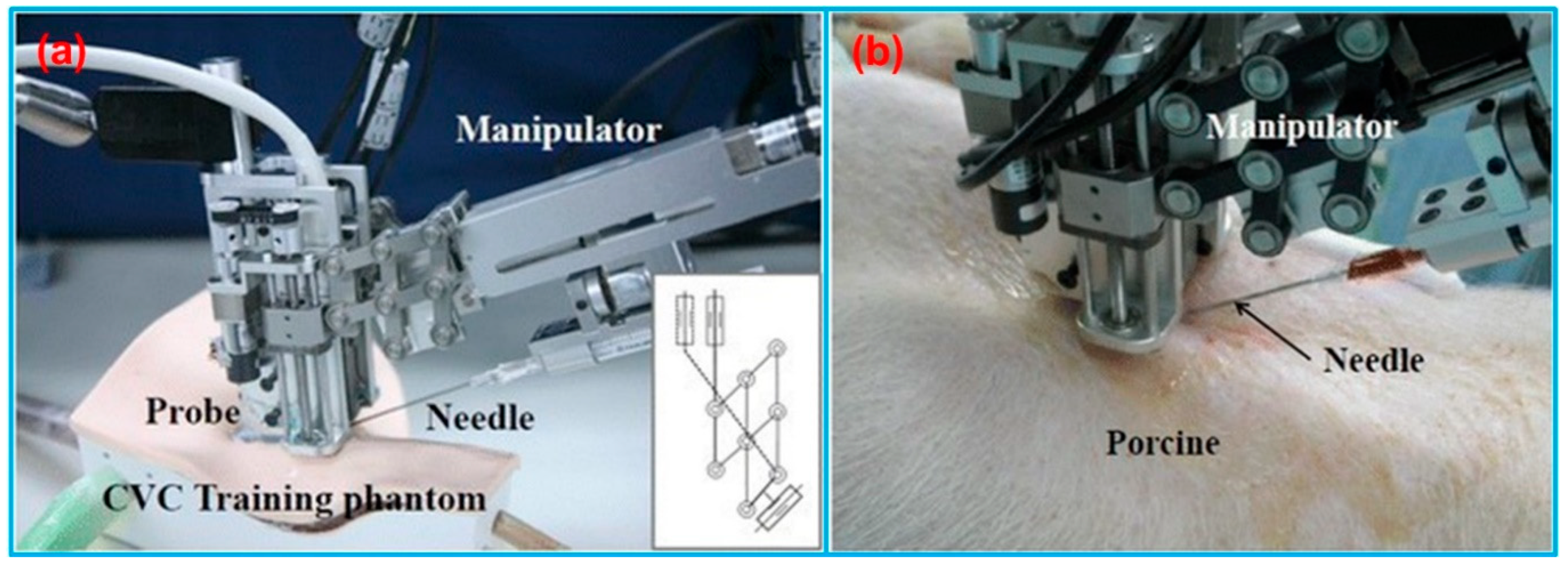
- Kobayashi, Y.; Hamano, R.; Watanabe, H.; Koike, T.; Hong, J.; Toyoda, K.; Uemura, M.; Ieiri, S.; Tomikawa, M.; Ohdaira, T. Preliminary in Vivo Evaluation of a Needle Insertion Manipulator for Central Venous Catheterization. ROBOMECH J. 2014, 1, 1–7. [Google Scholar] [CrossRef]


| Manufacturer | Model | Measurement Volume (Radius × Width × Height) or FOV | Resolution | Volumetric Accuracy (RMS) | Average Latency | Measurement Rate |
|---|---|---|---|---|---|---|
| Northern Digital Inc., Waterloo, ON, Canada | Polaris Vega ST [31] | 2400 × 1566 × 1312 mm3 (Pyramid Volume:) 3000 × 1856 × 1470 mm3 (Extended Pyramid) | N/A | 0.12 mm (Pyramid Volume) 0.15 mm (Extended Pyramid) | <16 ms | 60 Hz |
| Polaris Vega VT [32] | 2400 × 1566 × 1312 mm3 (Pyramid Volume) 3000 × 1856 × 1470 mm3 (Extended Pyramid) | N/A | 0.12 mm (Pyramid Volume) 0.15 mm (Extended Pyramid) | <16 ms | 60 Hz | |
| Polaris Vega XT [33] | 2400 × 1566 × 1312 mm3 (Pyramid Volume) 3000 × 1856 × 1470 mm3 (Extended Pyramid) | N/A | 0.12 mm (Pyramid Volume) 0.15 mm (Extended Pyramid) | <3 ms | 400 Hz | |
| Polaris Vicra [34] | 1336 × 938 × 887 mm3 | N/A | 0.25 mm | N/A | 20 Hz | |
| ClaroNav Inc., Toronto, ON, Canada | H3-60 [35] | 2400 × 2000 × 1600 mm3 | 1280 × 960 | 0.20 mm | ~60 ms | 16 Hz |
| SX60 [35] | 1150 × 700 × 550 mm3 | 640 × 480 | 0.25 mm | ~20 ms | 48 Hz | |
| HX40 [35] | 1200 × 1200 × 900 mm3 | 1024 × 768 | 0.20 mm | ~50 ms | 20 Hz | |
| HX60 [35] | 2000 × 1300 × 1000 mm3 | 1024 × 768 | 0.35 mm | ~50 ms | 20 Hz | |
| BTS Bioengineering Corp., Quincy, MA, USA | SMART DX 100 [36] | 2000 × 2000 × 2000 mm3 | 0.3 MP | <0.20 mm | N/A | 280 FPS |
| SMART DX 400 [36] | 4000 × 3000 × 3000 mm3 | 1.0 MP | <0.30 mm | N/A | 300 FPS | |
| SMART DX 700 [36] | 4000 × 3000 × 3000 mm3 | 1.5 MP | <0.10 mm | N/A | 1000 FPS | |
| SMART DX 6000 [36] | 4000 × 3000 × 3000 mm3 | 2.2 MP | <0.10 mm | N/A | 2000 FPS | |
| SMART DX 7000 [36] | 6000 × 3000 × 3000 mm3 | 4.0 MP | <0.10 mm | N/A | 2000 FPS | |
| NaturalPoint, Inc., Corvallis, OR, USA | OptiTrack PrimeX 41 [37] | FOV 51° × 51° | 4.1 MP | 0.10 mm | 5.5 ms | 250+ FPS |
| OptiTrack PrimeX 22 [38] | FOV 79° × 47° | 2.2 MP | 0.15 mm | 2.8 ms | 500+ FPS | |
| OptiTrack PrimeX 13 [39] | FOV 56° × 46° | 1.3 MP | 0.20 mm | 4.2 ms | 1000 FPS | |
| OptiTrack PrimeX 13W [40] | FOV 82° × 70° | 1.3 MP | 0.30 mm | 4.2 ms | 1000 FPS | |
| OptiTrack SlimX 13 [41] | FOV 82° × 70° | 1.3 MP | 0.30 mm | 4.2 ms | 1000 FPS | |
| OptiTrack V120: Trio [42] | FOV 47° × 43° | 640 × 480 | N/A | 8.33 ms | 120 FPS | |
| OptiTrack V120: Duo [43] | FOV 47° × 43° | 640 × 480 | N/A | 8.33 ms | 120 FPS | |
| OptiTrack Flex 13 [44] | FOV 56° × 46° | 1.3 MP | N/A | 8.3 ms | 120 FPS | |
| OptiTrack Flex 3 [45] | FOV 58° × 45° | 640 × 480 | N/A | 10 ms | 100 FPS | |
| OptiTrack Slim 3U [46] | FOV 58° × 45° | 640 × 480 | N/A | 8.33 ms | 120 FPS | |
| TrackIR 4 [47] | 46° (Horizontal) | 355 × 288 | N/A | N/A | 120 FPS | |
| TrackIR 5 [47] | 51.7° (Horizontal) | 640 × 480 | N/A | N/A | 120 FPS | |
| Qualisys Inc., Gothenburg, Sweden | Arqus A5 [30] | FOV 77° × 62° | 5 MP (normal) 1MP (high-speed) | 0.06 mm | N/A | 700 FPS (normal) 1400 FPS (high-speed) |
| Arqus A9 [30] | FOV 82° × 48° | 9 MP (normal) 2.5 MP (high-speed) | 0.05 mm | N/A | 300 FPS (normal) 590 FPS (high-speed) | |
| Arqus A12 [30] | FOV 70° × 56° | 12 MP (normal) 3 MP (high-speed) | 0.04 mm | N/A | 300 FPS (normal) 1040 FPS (high-speed) | |
| Arqus A26 [30] | FOV 77° × 77° | 26 MP (normal) 6.5 MP (high-speed) | 0.03 mm | N/A | 150 FPS (normal) 290 FPS (high-speed) | |
| Miqus M1 [48] | FOV 58° × 40° | 1 MP | 0.14 mm | N/A | 250 FPS | |
| Miqus M3 [48] | FOV 80° × 53° | 2 MP (normal) 0.5 MP (high-speed) | 0.11 mm | N/A | 340 FPS (normal) 650 FPS (high-speed) | |
| Miqus M5 [48] | FOV 49° × 49° | 4 MP (normal) 1 MP (high-speed) | 0.07 mm | N/A | 180 FPS (normal) 360 FPS (high-speed) | |
| Miqus Hybrid [49] | FOV 62° × 37° | 2 MP | N/A | N/A | 340 FPS | |
| 3+ [50] | N/A | 1.3 MP (normal) 0.3 MP (high-speed) | N/A | N/A | 500 FPS (normal) 1750 FPS (high-speed) | |
| 5+ [50] | 49° (Horizontal) | 4 MP (normal) 1 MP (high-speed) | N/A | N/A | 180 FPS (normal) 360 FPS (high-speed) | |
| 6+ [50] | 56° (Horizontal) | 6 MP (normal) 1.5 MP (high-speed) | N/A | N/A | 450 FPS (normal) 1660 FPS (high-speed) | |
| 7+ [50] | 54° (Horizontal) | 12 MP (normal) 3 MP (high-speed) | N/A | N/A | 300 FPS (normal) 1100 FPS (high-speed) | |
| Vicon Industries Inc., Hauppauge, NY, USA | Valkyrie VK26 [51] | FOV 72° × 72° | 26.2 MP | N/A | N/A | 150 FPS |
| Valkyrie VK16 [51] | FOV 72° × 56° | 16.1 MP | N/A | N/A | 300 FPS | |
| Valkyrie VK8 [51] | FOV 72° × 42° | 8.0 MP | N/A | N/A | 500 FPS | |
| Valkyrie VKX [51] | FOV 66° × 66° | 7.2 MP | N/A | N/A | 380 FPS | |
| Vantage+ V16 [52] | FOV 76.4° × 76.4° | 16 MP (normal) 4.2 MP (high-speed) | N/A | 8.3 ms | 120 FPS (normal) 500 FPS (high-speed) | |
| Vantage+ V8 [52] | FOV 61.7° × 47° | 8 MP (normal) 2.2 MP (high-speed) | N/A | 5.5 ms | 260 FPS (normal) 910 FPS (high-speed) | |
| Vantage+ V5 [52] | FOV 63.5° × 55.1° | 5 MP (normal) 1.8 MP (high-speed) | N/A | 4.7 ms | 420 FPS (normal) 1070 FPS (high-speed) | |
| Vero v2.2 [53] | FOV 98.1° × 50.1° | 2.2 MP | N/A | 3.6 ms | 330 FPS | |
| Vero v1.3 [53] | FOV 55.2° × 43.9° | 1.3 MP | N/A | 3.4 ms | 250 FPS | |
| Vero v1.3 X [53] | FOV 79.0° × 67.6° | 1.3 MP | N/A | 3.4 ms | 250 FPS | |
| Vero Vertex [53] | FOV 100.6° × 81.1° | 1.3 MP | N/A | 3.4 ms | 120 FPS | |
| Vue [54] | FOV 82.7° × 52.7° | 2.1 MP | N/A | N/A | 60 FPS | |
| Viper [55] | FOV 81.8° × 49.4° | 2.2 MP | N/A | 3.2 ms | 240 FPS | |
| ViperX [56] | FOV 50.2° × 50.2° | 6.3 MP | N/A | 3.2 ms | 240 FPS | |
| Atracsys LLC., Puidoux, Switzerland | fusionTrack 500 [57] | 2000 × 1327 × 976 mm3 | 2.2 MP | 0.09 mm | ~ 4 ms | 335 Hz |
| fusionTrack 250 [58] | 1400 × 1152 × 900 mm3 | 2.2 MP | 0.09 mm | ~ 4 ms | 120 Hz | |
| spryTrack 180 [59] | 1400 × 1189 × 1080 mm3 | 1.2 MP | 0.19 mm | <25 ms | 54 Hz | |
| spryTrack 300 [60] | 1400 × 805 × 671 mm3 | 1.2 MP | 0.14 mm | <25 ms | 54 Hz | |
| Motion Analysis Corp., Rohnert Park, CA, USA | Kestrel 4200 [61] | N/A | 4.2 MP | N/A | N/A | 200 FPS |
| Kestrel 2200 [62] | N/A | 2.2 MP | N/A | N/A | 332 FPS | |
| Kestrel 1300 [63] | N/A | 1.3 MP | N/A | N/A | 204 FPS | |
| Kestrel 300 [64] | N/A | 0.3 MP | N/A | N/A | 810 FPS | |
| STT Systems, Donostia-San Sebastian, Spain | EDDO Biomechanics [65] | N/A | N/A | 1 mm | N/A | 120 FPS |
| Advanced Realtime Tracking GmbH & Co. KG, Oberbayern, Germany | ARTTRACK6/M [66] | FOV 135° × 102° | 1280 × 1024 | N/A | N/A | 180 Hz |
| ARTTRACK5 [67] | FOV 98° × 77° | 1280 × 1024 | N/A | 10 ms | 150 Hz | |
| SMARTTRACK3 [68] | FOV 135° × 102° | 1280 × 1024 | N/A | 9 ms | 150 Hz |
| Manufacturer | Model | Tracking Distance | Position Accuracy (RMS) | Orientation Accuracy (RMS) | Average Latency | Measurement Rate |
|---|---|---|---|---|---|---|
| Northern Digital Inc., Waterloo, ON, Canada | Aurora-Cube Volume-5DOF [70] | N/A | 0.70 mm | 0.2° | N/A | 40 Hz |
| Aurora-Cube Volume-6DOF [70] | N/A | 0.48 mm | 0.3° | N/A | 40 Hz | |
| Aurora-Dome Volume-5DOF [70] | 660 mm | 1.10 mm | 0.2° | N/A | 40 Hz | |
| Aurora-Dome Volume-6DOF [70] | 660 mm | 0.70 mm | 0.3° | N/A | 40 Hz | |
| 3D Guidance trakSTAR-6DOF [71] | 660 mm | 1.40 mm | 0.5° | N/A | 80 Hz | |
| 3D Guidance driveBAY-6DOF [71] | 660 mm | 1.40 mm | 0.5° | N/A | 80 Hz | |
| Polhemus Inc., Colchester, VT, USA | Viper [72] | N/A | 0.38 mm | 0.10° | 1 ms | 960 Hz |
| Fastrak [73] | N/A | 0.76 mm | 0.15° | 4 ms | 120 Hz | |
| Patriot [74] | N/A | 1.52 mm | 0.40° | 18.5 ms | 60 Hz | |
| Patriot Wireless [75] | N/A | 7.62 mm | 1.00° | 20 ms | 50 Hz | |
| Liberty [76] | N/A | 0.76 mm | 0.15° | 3.5 ms | 240 Hz | |
| Liberty Latus [77] | N/A | 2.54 mm | 0.50° | 5 ms | 188 Hz | |
| G4 [78] | N/A | 2.00 mm | 0.50° | <10 ms | 120 Hz |
| Manufacturer | Model | Static Accuracy (Roll/Pitch) | Static Accuracy (Heading) | Dynamic Accuracy (Roll/Pitch) | Dynamic Accuracy (Heading) | Average Latency | Update Rate |
|---|---|---|---|---|---|---|---|
| Xsens Technologies B.V., Enschede, The Netherlands | MTw Awinda [82] | 0.5° | 1.0° | 0.75° | 1.5° | 30 ms | 120 Hz |
| Xsens DOT [81] | 0.5° | 1.0° | 1.0° | 2.0° | 30 ms | 60 Hz | |
| MTi-1 [83] | 0.5° | N/A | N/A | N/A | N/A | 100 Hz | |
| MTi-2 [83] | 0.5° | N/A | 0.8° | N/A | N/A | 100 Hz | |
| MTi-3 [83] | 0.5° | N/A | 0.8° | 2.0° | N/A | 100 Hz | |
| MTi-7 [83] | 0.5° | N/A | 0.5° | 1.5° | N/A | 100 Hz | |
| MTi-8 [83] | 0.5° | N/A | 0.5° | 1.0° | N/A | 100 Hz | |
| MTi-20 [84] | 0.2° | N/A | 0.5° | N/A | N/A | N/A | |
| MTi-30 [84] | 0.2° | N/A | 0.5° | 1.0° | N/A | N/A | |
| MTi-200 [84] | 0.2° | N/A | 0.3° | N/A | <10 ms | N/A | |
| MTi-300 [84] | 0.2° | N/A | 0.3° | 1.0° | <10 ms | N/A | |
| MTi-710 [84] | 0.2° | N/A | 0.3° | 0.8° | <10 ms | 400 Hz | |
| MTi-610 [85] | N/A | N/A | N/A | N/A | N/A | 400 Hz | |
| MTi-620 [85] | 0.2° | N/A | 0.25° | N/A | N/A | 400 Hz | |
| MTi-630 [85] | 0.2° | N/A | 0.25° | 1.0° | N/A | 400 Hz | |
| MTi-670 [85] | 0.2° | N/A | 0.25° | 0.8° | N/A | 400 Hz | |
| MTi-680 [85] | 0.2° | N/A | 0.25° | 0.5° | N/A | 400 Hz | |
| STT Systems, Donostia-San Sebastian, Spain | iSen system [86] | N/A | N/A | <0.5° | <2.0° | N/A | 400 Hz |
| VectorNav Technologies, Dallas, TX, USA | VN-100 [87] | 0.5° | N/A | 1.0° | 2.0° | N/A | 800 Hz |
| VN-110 [88] | 0.05° | N/A | N/A | 2.0° | N/A | 800 Hz | |
| VN-200 [89] | 0.5° | 2.0° | 0.2°, 1σ | 0.03°, 1σ | N/A | 800 Hz | |
| VN-210 [90] | 0.05° | 2.0° | 0.015°, 1σ | 0.05–0.1°, 1σ | N/A | 800 Hz | |
| VN-300 [91] | 0.5° | 2.0° | 0.03°, 1σ | 0.2°, 1σ | N/A | 400 Hz | |
| VN-310 [92] | 0.05° | 2.0° | 0.015°, 1σ | 0.05–0.1°, 1σ | N/A | 800 Hz | |
| Advanced Navigation, Sydney, Australia | Motus [93] | 0.05° | 0.8° | N/A | N/A | N/A | 1000 Hz |
| Orientus [94] | 0.2° | 0.8° | 0.6° | 1.0° | 0.3 ms | 1000 Hz | |
| Boreas D90 [95] | 0.005° * | 0.006° * | N/A | N/A | N/A | 1000 Hz | |
| Spatial FOG Dual [96] | 0.005° * | 0.007° | N/A | N/A | N/A | 1000 Hz | |
| Certus Evo [97] | 0.01° * | 0.01° | N/A | N/A | N/A | 1000 Hz | |
| Certus [98] | 0.03° * | 0.06° | N/A | N/A | N/A | 1000 Hz | |
| Spatial [99] | 0.04° * | 0.08° | N/A | N/A | 0.4 ms | 1000 Hz | |
| GNSS Compass [100] | 0.4° | 0.4° | N/A | N/A | N/A | 200 Hz | |
| Inertial Labs, Paeonian Springs, VA, USA | KERNEL-100 [101] | 0.05° | 0.08° | N/A | N/A | <1 ms | 2000 Hz |
| KERNEL-110 [102] | 0.05° | 0.08° | N/A | N/A | <1 ms | 2000 Hz | |
| KERNEL-120 [102] | 0.05° | 0.08° | N/A | N/A | <1 ms | 2000 Hz | |
| KERNEL-210 [103] | 0.05° | 0.08° | N/A | N/A | <1 ms | 2000 Hz | |
| KERNEL-220 [103] | 0.05° | 0.08° | N/A | N/A | <1 ms | 2000 Hz | |
| IMU-P [104] | 0.05° | 0.08° | N/A | N/A | <1 ms | 2000 Hz |
| System Type | Manufacturer | Year of FDA Approval | US Image Acquisition | Tracking Principle | Biopsy Route |
|---|---|---|---|---|---|
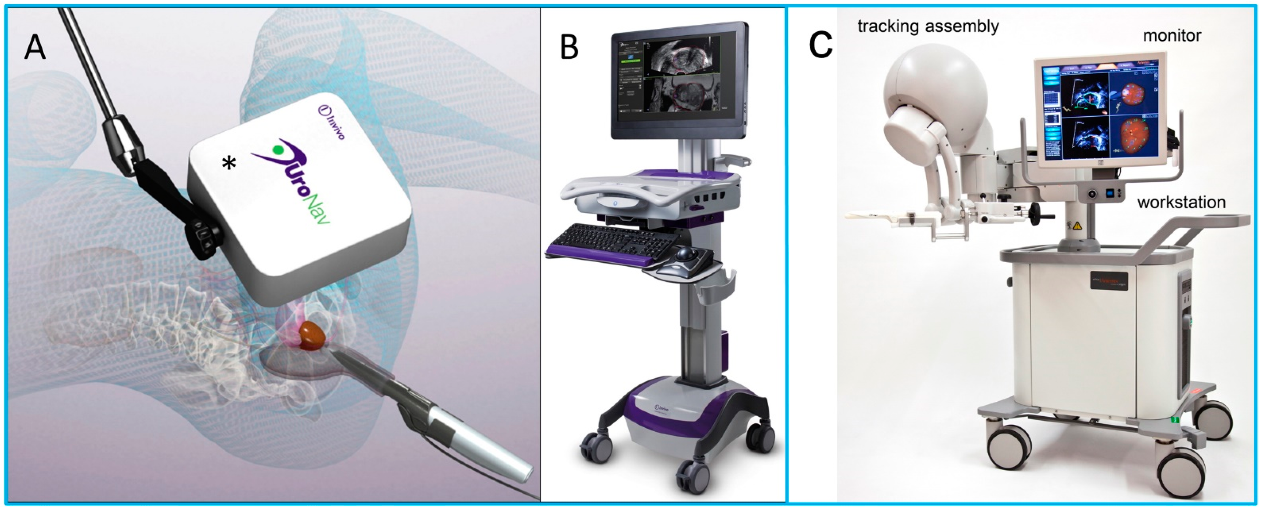
| UroNav | Philips | 2005 | Manual sweep | Electromagnetic tracking | Transrectal |
| Artemis | Eigen | 2008 | Manual rotation | Mechanical arm | Transrectal |
| Urostation | Koelis | 2010 | Automatic US probe rotation | Real-time registration | Transrectal |
| HI-RVS | Hitachi | 2010 | Real-time biplanar transrectal US | Electromagnetic tracking | Transrectal or transperineal |
| GeoScan | BioJet | 2012 | Manual sweep | Mechanical arm | Transrectal or transperineal |
| Reference | Modality for Fusion | Tracking Principle | Application |
|---|---|---|---|
| Park et al. [148] | Liver CT or MRI | Electromagnetic tracking | Biopsy of focal hepatic lesions with poor conspicuity on conventional B-mode US image |
| Lee et al. [149] | Liver CT or MRI | Electromagnetic tracking | Lesion detection of small hepatocellular carcinomas (HCCs) |
| Song et al. [150] | Liver CT or MRI | Plane registration and point registration | Improve sonographic conspicuity of HCC and feasibility of percutaneous radiofrequency ablation for HCCs not visible on conventional US images |
| Helck et al. [151] | Renal CT or MRI | Electromagnetic tracking | Identifiability and assessment of the dignity of renal lesions |
| Andersson et al. [152] | Renal CT | Electromagnetic tracking | Image-guided percutaneous radiofrequency ablation of small renal masses |
| Zhang et al. [153] | Pancreatic CT | Real-time registration | Image-guided percutaneous catheter drainage in treatment of acute pancreatitis |
| Klauser et al. [143] | Musculoskeletal CT | Internal landmarks | Image-guided sacroiliac joint injection |
| Lee et al. [141] | Thigh MRI | Real-time registration | Selecting the appropriate biopsy site in patients with suspected myopathies |
| Rubenthaler et al. [154] | Renal MRI/contrast enhanced US | Electromagnetic tracking | Classification of unclear and difficult renal lesions |
Publisher’s Note: MDPI stays neutral with regard to jurisdictional claims in published maps and institutional affiliations. |
© 2022 by the authors. Licensee MDPI, Basel, Switzerland. This article is an open access article distributed under the terms and conditions of the Creative Commons Attribution (CC BY) license (https://creativecommons.org/licenses/by/4.0/).
Share and Cite
Peng, C.; Cai, Q.; Chen, M.; Jiang, X. Recent Advances in Tracking Devices for Biomedical Ultrasound Imaging Applications. Micromachines 2022, 13, 1855. https://doi.org/10.3390/mi13111855
Peng C, Cai Q, Chen M, Jiang X. Recent Advances in Tracking Devices for Biomedical Ultrasound Imaging Applications. Micromachines. 2022; 13(11):1855. https://doi.org/10.3390/mi13111855
Chicago/Turabian StylePeng, Chang, Qianqian Cai, Mengyue Chen, and Xiaoning Jiang. 2022. "Recent Advances in Tracking Devices for Biomedical Ultrasound Imaging Applications" Micromachines 13, no. 11: 1855. https://doi.org/10.3390/mi13111855