Orthogonality Measurement of Three-Axis Motion Trajectories for Micromanipulation Robot Systems

Abstract

In robotic micromanipulation systems, the orthogonality of the three-axis motion trajectories of the motion control systems influences the accuracy of micromanipulation. A method of measuring and evaluating the orthogonality of three-axis motion trajectories is proposed in this paper. Firstly, a system for three-axis motion trajectory measurement is developed and an orthogonal reference coordinate system is designed. The influence of the assembly error of laser displacement sensors on the reference coordinate system is analyzed using simulation. An approach to estimating the orthogonality of three-axis motion trajectories and to compensating for its error is presented using spatial line fitting and vector operation. The simulation results show that when the assembly angle of the laser displacement sensors is limited within a range of 10°, the relative angle deviation of the coordinate axes of the reference coordinate frame is approximately 0.09%. The experiment results show that precision of spatial line fitting is approximately 0.02 mm and relative error of the orthogonality measurement is approximately 0.3%.

1. Introduction

Stereo light microscopes (SLMs) consist of two independent optical paths that form a binocular microscopic stereovision system. This kind of stereovision system not only possesses a long working distance, but can also capture dynamic-scene images in real time. Therefore, it is suitable for microscopic fields, and it can be combined with motion control systems and micromanipulators to form automatic micromanipulation robot systems, which are employed to capture, transfer, or assemble some microscale objects (such as biological tissues, cells, microstructures, etc.). Their sizes range from microns to submillimeter, and the positioning precision of the system can reach micron or even submicron or nanometer levels. This kind of system has been applied in microassembly [1,2,3], microinjection [4,5], bioengineering [6,7,8,9,10,11], minimally invasive surgery [12,13,14,15], and other microscopic fields. The motion control system with three translational degrees of freedom and driven by ball screw, guide rail, slider, and motor, is one of the various motion control systems. It has a simple structure, can provide small displacement in three orthogonal directions, and can drive the micromanipulator to move in a small length range. Its control program design is flexible, and the displacement can be adjusted under various resolutions. This kind of motion control system is convenient to use in micromanipulation robot systems [16,17]. It contains three motion axes, which are equivalent to the three axes in the Cartesian coordinate system. Theoretically, when moving along these three axes or in the same direction, their trajectories should be straight lines and orthogonal to each other. The better the linearity and orthogonality of the motion trajectory lines on the motion axes, the higher the positioning precision. However, due to the machining accuracy of the ball screw and other transmission errors, the real motion control system cannot achieve absolute orthogonality and straightness of the motion trajectory. Therefore, these two factors need to be measured and corrected in high-precision micromanipulation robot systems.

The basic unit of a motion control system is the linear motion module. One-dimensional linear motion modules are composed of a ball screw, guide rail, and motor. According to the orthogonal assembly relationship, three motion modules are combined to form a three-axis motion control system. The positioning precision of this motion control system is inevitably affected by the machining accuracy of main parts such as ball screw and guide rail. Considerable research has been conducted on the error source, error distribution, error modeling, error analysis, and error compensation of the ball screw and guide rail [18,19,20,21,22]. Before leaving the factory, the manufacturer usually conducts orthogonal experiments on the linear motion module assembly using auxiliary tools such angle rulers and angle measuring instruments to measure the installation angles between the linear motion modules to ensure the orthogonal relationship of installation angles much far as possible. However, in the motion process, the three-axis linear motion module group is affected by a variety of error sources (such as the machining precision of ball screws and guide rails; the transmission error between ball screws, guide rails, and sliders; the assembly’s orthogonal error; etc.), so its trajectories on three motion axes are not strictly in a straight line and orthogonal. Especially when these linear motion modules are integrated into the micromanipulation robot system, they need to be reassembled, which will break the original assembly relationship. Therefore, in micromanipulation robot systems with high precision positioning requirements, the trajectories of the motion axes are measured by obtaining the position coordinates of points on the motion trajectories, and the orthogonality and straightness of the trajectories of the motion axes are analyzed to provide data for the calibration of the orthogonality and straightness of the motion axis, which are helpful for improving the positioning precision of motion control systems.

Laser interferometry methods can be used for length measurement in precision environments [23,24]. They use the principle of light interference to generate interference fringes. By analyzing the patterns of interference fringes to measure the distance, high measurement accuracy can be achieved (nanometer and micron levels, etc.). For example, these methods are used to measure and compensate for the geometric error and nonlinear force error of high-speed, high-precision, and large-scale motion control system of mounters [25]. When using laser interferometry to measure the error of the motion control system, the measurement and compensation accuracy can reach the micron level. Laser interferometry methods can also be used for position tracking and measurement of three-axis motion control systems with a ball screw and motor, but the cost of the interference measurement equipment is high and the equipment requires sufficient installation space. The binocular stereo vision method can also be used to track spatial position and measure trajectory [26,27]. A calibration object is mounted on the three-axis motion control system to make the calibration object move along the three motion axes. The stereo image pairs of the calibration object are obtained by a binocular camera. The motion trajectories of the calibration object can be reconstructed based on stereo matching and visual calculation. This kind of measurement system is easy to build, low cost, and easy to use, but the measurement accuracy depends on the accuracy of image processing and stereo vision calculation. In recent years, laser displacement sensors based on the principle of triangulation have developed rapidly, with the emergence of point sensors, stripe-structured light sensors, etc., which can detect the position of a single point or multiple simultaneously and are being increasingly widely used for many tasks such as shape reconstruction, geometric dimension measurement, distance measurement, etc. [28,29,30,31]. The design of the laser displacement sensor is modularized and compact. It can provide displacement data of different ranges and precisions; it is also cheap and a compact position tracking and measurement system is easy to build. The working space of the micromanipulation robot system is narrow and small, and the system for measuring the trajectory of the motion axis is required to have a small and compact structure, so laser displacement sensors are suitable for this demand.

Focusing on the three-axis motion control system used in micromanipulation robot systems, the purpose of this study was to construct a method to measure and analyze the orthogonality and linearity of the trajectories of the motion axes. Based on a laser displacement sensor with a small spot, a spatial position tracking system was designed to measure the trajectories of the motion axes. On this basis, an evaluation method of the orthogonality and linearity of the trajectory of the motion axis was established. The method is low-cost, easy to use, and suitable for micromanipulation. In addition, it can be used as an on-site measurement system without too much calibration. Because laser displacement sensors are general module that have a variety of ranges and precision, the method can also meet different range and precision requirements (such as submicron, micron, tens of microns, etc.), which is very flexible.

The remainder of this article is organized as follows: In Section 2, the micromanipulation robot system is introduced; in Section 3, the method for three-axis orthogonality measurement is developed. In Section 4, the orthogonal reference coordinate system is analyzed. This method is discussed in Section 5, and the conclusions are described in Section 6.

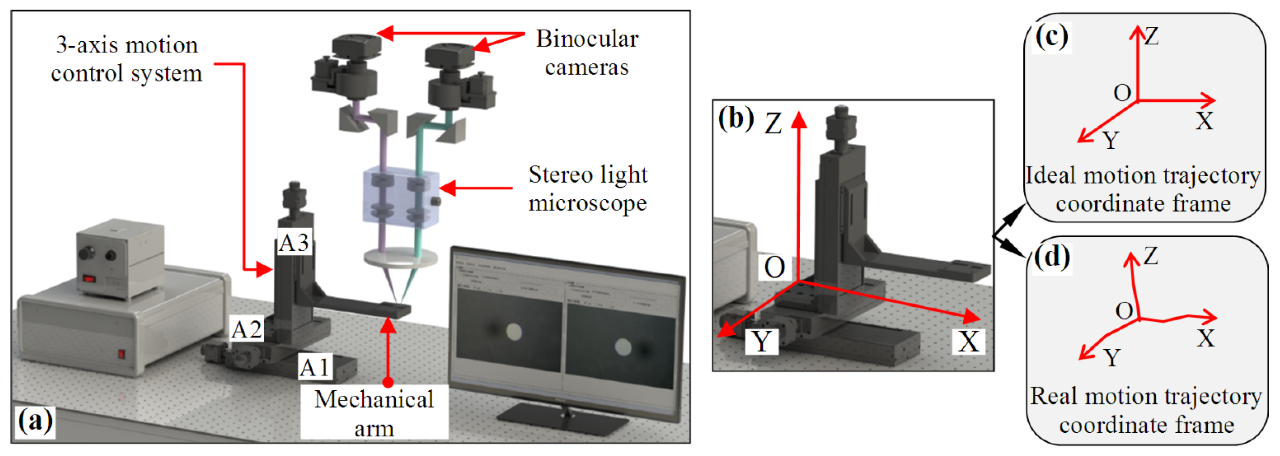
2. Motion Trajectory Coordinate Frame

Figure 1a shows a special robotic micromanipulation system [16,17,26] that uses a stereo light microscope and binocular cameras to form a microscopic binocular stereovision system, which captures stereo image pairs of space scene in real time, and realizes three-dimensional positioning, navigation, position feedback, etc. In this system, the three-axis motion control system is used as the positioning driver, which receives the position coordinates reconstructed by the binocular stereovision system to achieve accurate positioning. Various types of micromanipulators can be carried on its mechanical arm to perform tasks such as microgripping, microassembly, microinjection, etc. The three-axis motion control system is used not only as the coordinate acquisition device of control points for system calibration, but also as the driving device of position adjustment.

The three-axis motion control system in Figure 1a is composed of three linear motion modules, which are assembled according to the orthogonal relationship. Each linear motion module is mainly composed of a ball screw, double linear guide, coupling, and a motor. To describe the position coordinates of the three-axis motion control system in the motion process, the motion trajectory coordinate frame is defined as shown in Figure 1b. The motion trajectory coordinate frame is represented by O-XYZ, where O is the origin, and X, Y, and Z represent the three motion coordinate axes. At the starting position of each linear motion module, a triggered switch sensor is installed to generate an absolute zero point (or the zero point of grating ruler installed on linear motion module is used as the zero point of the module), and the position of the absolute zero points of the three motion modules is used as the origin of the coordinate frame, i.e., point O. The trajectories of the three motion axes are generated as follows: At one time, only one linear motion module is allowed to move in a line, and the other two linear motion modules remain stationary. The trajectory of the moving module forms a motion coordinate axis. According to this rule, modules A1, A2, and A3 move in a line separately, and their trajectories form the three motion coordinate axes: X-, Y-, and Z-axes. If none of the error factors interfere with the motion, the trajectory lines of the X-, Y-, and Z-axes should be lines; after the three linear motion modules are assembled according to the orthogonal relationship, the trajectory lines of the three motion axes are orthogonal, so the motion coordinate frame at this time is a typical Cartesian coordinate frame, as shown in Figure 1c. However, the motion control system is actually affected by a variety of error factors in the motion process such as: (1) when the vertical installation angles between the three linear motion modules deviate 90°, the motion trajectory lines on the X-, Y-, and Z-axes cannot guarantee perpendicularity. In the assembly process, this error factor will only be reduced as much as possible, but will not disappear. (2) The machining precision of the ball screw and guide rail affects the straightness of the motion trajectory on the X-axis, the Y-axis and the Z-axis, which may cause small deformation of the motion trajectory line. This error source also affects the orthogonality of the motion trajectory line. (3) The assembly error among the ball screw, guide rail, and slider also affects the linearity and orthogonality of motion trajectory line on the motion coordinate axis. Only a few error sources are introduced above, but their effects do exist. Due to the influence of error factors, the motion trajectory coordinate frame is no longer a Cartesian coordinate frame in terms of orthogonality and coordinate axis linearity, as shown in Figure 1d. The posture of deviation from orthogonality and line is relatively small. It is not necessary to analyze and correct the orthogonality and coordinate axis linearity for all three-axis motion control systems, only when there is a need for high-precision positioning is this analysis is more necessary, such as the system in Figure 1a.

The motion of the three-axis motion control system is realized by a control algorithm, which is designed based on the Cartesian coordinate frame in Figure 1c. It can be imagined that when the three-axis motion control system moves in the coordinate frame in Figure 1d, it cannot accurately reach the preset position by the control algorithm, so for the system in Figure 1a, it is necessary to analyze the orthogonality and linearity of the motion trajectory coordinates. Therefore, we developed an orthogonality and linearity evaluation method.

3. Methods

A schematic diagram of three-axis motion trajectory measurement is shown in Figure 2. Three grating-ruler sensors with a resolution of 0.1 μm were precisely installed on the X, Y, and Z linear motion modules of the motion control system to measure small displacement in each motion axis. The origin of the motion trajectory coordinate frame O-XYZ was set on the motion control system, and the X-, Y-, and Z-axes coincided with the motion trajectories of the three linear motion modules. The motion trajectories can be regarded as a series of spatial discrete points, whose spatial coordinates are obtained by the measurement system, as shown in Figure 2. A cuboid gauge block composed of stainless steel was installed on the motion control system, and its three adjacent surfaces, A, B, and C, were used as the test surfaces for displacement measurement. These test surfaces had good surface roughness and maintained accurate orthogonality.

When assembling the gauge block, the normal direction of its three test surfaces should be parallel to the X-, Y-, and Z-axes as much as possible. That is, the normal directions of the three test surfaces A, B, and C should be parallel to the trajectory lines of the three motion axes of the motion control system as much as possible. The gauge block followed the motion control system; moved along the X-, Y-, and Z-axes at intervals; and stayed at the preset location for a certain time. Then, three laser displacement sensors (HG-C1050, Panasonic, Tokyo, Japan) were used to measure the displacement of the three test surfaces simultaneously. Three laser displacement sensors (A, B, and C) were used to construct the motion trajectory measurement system to measure the displacement of the three test surfaces (A, B, and C). During assembly of the three laser displacement sensors, the central-axis lines of the sensors should satisfy the orthogonal condition as much as possible. The non-orthogonality of laser sensor assembly influences the displacement measurement and is discussed in Section 4. The three laser displacement sensors constitute an approximate orthogonal world coordinate frame denoted by Q-UVW, where Q is the origin; U, V, and W represent the three axes; and the measured motion trajectories of the gauge block are described in Q-UVW. The spatial trajectory lines corresponding to the motion trajectories were obtained by the spatial linear fitting method, and the vector parameters of the spatial lines were derived from spatial line equations. Then, the angles between these spatial trajectory lines were calculated by vector calculation and the orthogonality of the three coordinate axes of O-XYZ were estimated. If the coordinate axes of O-XYZ do not satisfy the orthogonal conditions, it becomes a non-orthogonal coordinate frame and its coordinates should be corrected based on the orthogonality measurement. These coordinates in the real non-orthogonal O-XYZ are transformed into a virtual orthogonal coordinate system; then, accurate positioning control is achieved. The valid detection ranges of the three laser displacement sensors are depicted by dotted lines in Figure 2. The gauge block only moves in the valid space.

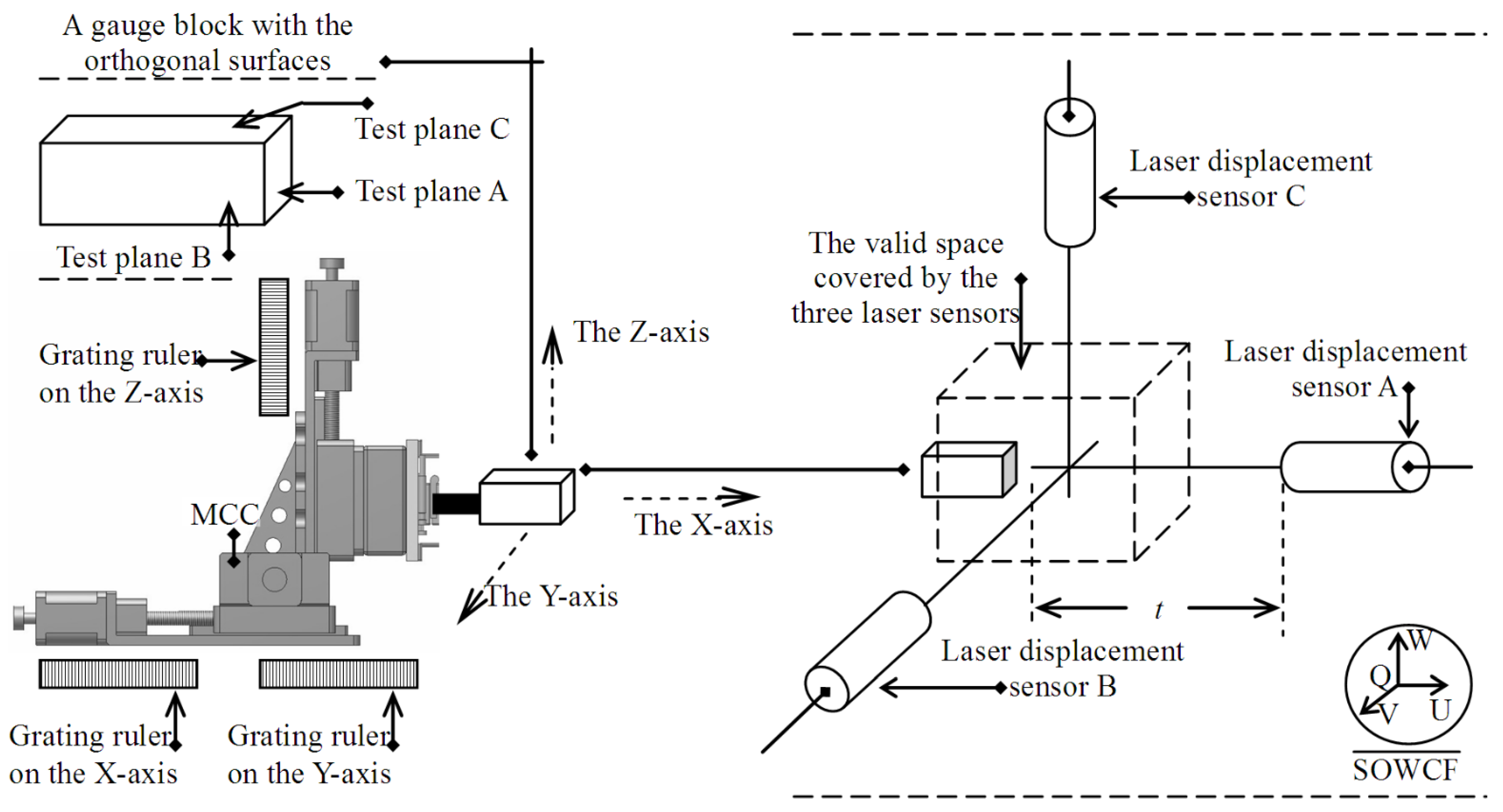
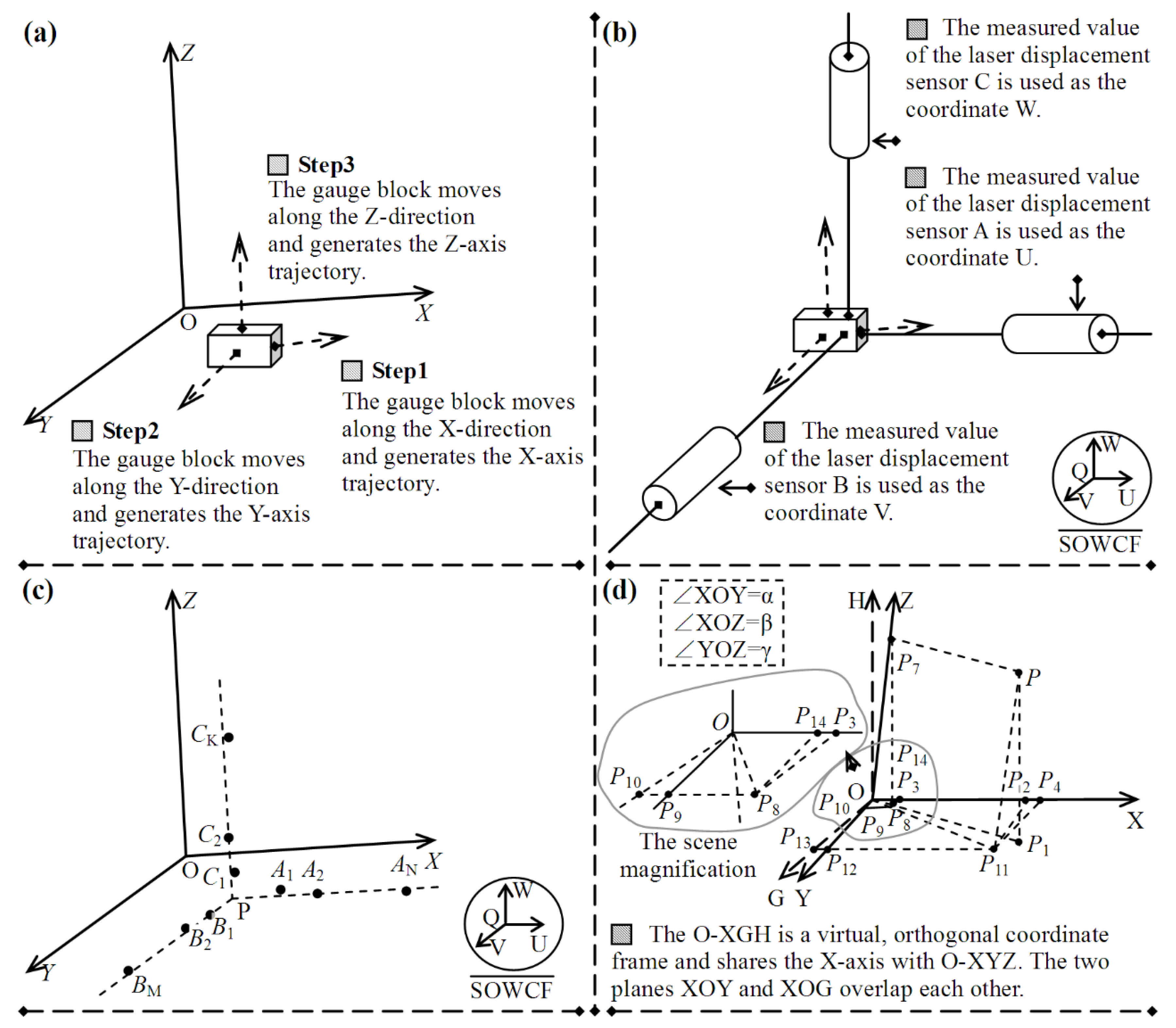
3.1. Data Acquisition

The three laser displacement sensors were used to construct the approximate orthogonal world coordinate frame Q-UVW, as shown in Figure 2. To measure the trajectories on the motion axes, the gauge block moved along the preset trajectories in the valid cuboid space, and the displacement of the test surface was measured. In Figure 2, S represents the vector of a point on the test surface in Q-UVW, and is generated by the laser displacement sensors; R represents its vector in O-XYZ, and is generated by the three grating-ruler sensors. The motion trajectory is composed of a series of separate points, and the coordinate vectors of all the separate points constitute a data sample, which is the basic data of the orthogonality estimation of the three-axis motion trajectories of O-XYZ. Figure 3 shows the acquisition of data samples.

The gauge block moved at preset distance intervals on the X-, Y-, and Z-axes, or in directions parallel to them. In Figure 2, {A_n|1 ≤ n ≤ N} represents the set consisting of N points on the X-axis trajectory and A_n is an element. Point A_n corresponds to two vectors: one is defined in O-XYZ, and the other is defined in Q-UVW. So, the set {A_n|1 ≤ n ≤ N} corresponds to two coordinate vector samples: {R_an = (x_an, y_an, z_an)^T|1 ≤ n ≤ N} and {S_an = (u_an, v_an, w_an)^T|1 ≤ n ≤ N}. The vector S_an consists of three elements, u_an, v_an, and w_an, whose values are the three displacement components of the gauge block at point A_n. S_an is measured by the three laser displacement sensors. Similarly, {B_m|1 ≤ m ≤ M} and {C_k|1 ≤ k ≤ K} are the point sets corresponding to the Y- and Z-axis trajectories, respectively, and their vector sets are {R_bm = (x_bm, y_bm, z_bm)^T|1 ≤ m ≤ M} and {S_bm = (u_bm, v_bm, w_bm)^T|1 ≤ m ≤ M}, respectively.

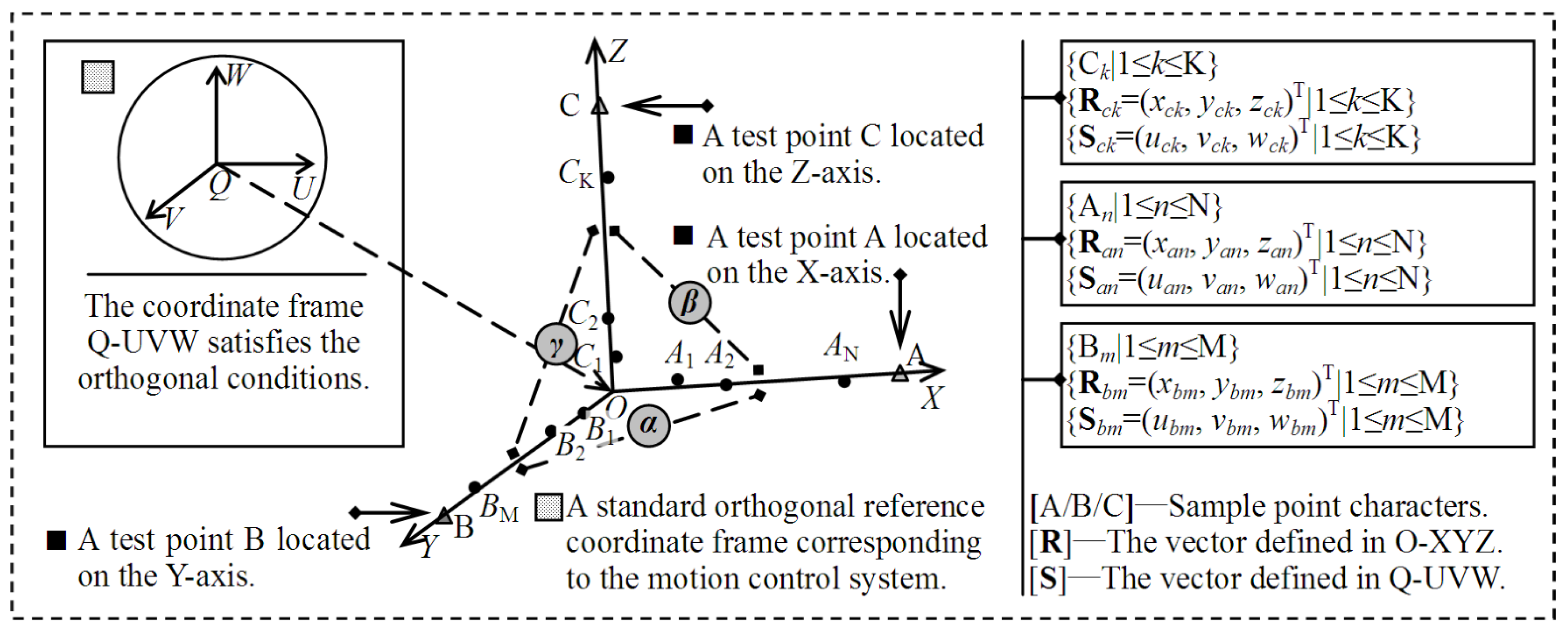
3.2. Three-Axis Orthogonality Evaluation

In this section, a spatial linear fitting approach is applied to the vector sets {S_an|1 ≤ n ≤ N}, {S_bm|1 ≤ m ≤ M}, and {S_ck|1 ≤ k ≤ K}, which outputs the line equations and their parameters. The intersection angles between the fitted lines are calculated based on vector operation, and the orthogonality of the fitted lines in O-XYZ is analyzed based on these angles. The intersection angles between the X- and Y-axis, between the X- and Z-axis, and between the Y- and Z-axis are denoted by α, β, and γ, respectively, as shown in Figure 3, the values of which indicate the orthogonal levels between the coordinate axes. The classification criteria related to the orthogonality are proposed and listed in

Table 1. The orthogonal rules defined for motion trajectory lines.

Category	α	β	γ	Logic
Orthogonal rule	|α-90°| ≤ Tabc	|β-90°| ≤ Tabc	|γ-90°| ≤ Tabc	α&β&γ
Non-orthogonal rule	|α-90°| > Tabc	|β-90°| > Tabc	|γ-90°| > Tabc	A||β||γ

where T_abc is a preset threshold for the angles α, β and γ.

.

The angles α, β, and γ are compared with 90°. The orthogonality condition is satisfied if the differences between these angles are less than the threshold T_abc; instead, the condition cannot be satisfied.

Figure 4 shows the process of the orthogonality estimation, which includes the following steps:

Step 1: The data acquisition process is conducted; the three sets are generated, {A_n|1 ≤ n ≤ N}, {B_m|1 ≤ m ≤ M}, and {C_k|1 ≤ k ≤ K}; and their vector sets are measured, as shown in Figure 4a,b.

Step 2: A spatial linear fitting approach is applied to the six vector samples in Figure 3. The linear equations and their parameters are obtained, and the error of spatial line fitting is calculated, as shown in Figure 4c.

Step 3: The angles α, β, and γ are calculated based on the parameters, and the orthogonality between the coordinate axes is analyzed on the basis of the principles defined in Table 1.

A general expression of spatial line equation is defined as follows:

$$\frac{u-u_0}{{\rho }_u}=\frac{v-v_0}{{\rho }_v}=\frac{w-w_0}{{\rho }_w}$$

(1)

where (u, v, w)^T is the coordinate vector of a point located in Q-UVW, (u₀, v₀, w₀)^T is the coordinate vector of a known reference point, and (ρ_u, ρ_v, ρ_w)^T is the unit vector of the spatial line. The above six parameters describe a spatial line and constitute a parameter vector P, where P = (u₀, v₀, w₀, ρ_u, ρ_v, ρ_w)^T. The fitted lines based on the three sets, {S_an|1 ≤ n ≤ N}, {S_bm|1 ≤ m ≤ M}, and {S_ck|1 ≤ k≤ K}, can be described by the following general expression:

$$\{\begin{array}{c}{P}_a=F\left(\left\{S_{an}|1\le n\le N\right\}\right)\hfill \\ P_b=F\left(\left\{S_{bm}|1\le m\le N\right\}\right)\hfill \\ P_c=F\left(\left\{S_{ck}|1\le k\le N\right\}\right)\hfill \end{array}$$

(2)

where F represents spatial line fitting method; P_a, P_b, and P_c are the three parameter vectors of P, where P_a = (u_0,a, v_0,a, w_0,a, ρ_u,a, ρ_v,a, ρ_w,a)^T, P_b = (u_0,b, v_0,b, w_0,b, ρ_u,b, ρ_v,b, ρ_w,b)^T, and P_c = (u_0,c, v_0,c, w_0,c, ρ_u,c, ρ_v,c, ρ_w,c)^T. Deng et al. [32] proposed a mixed least-square algorithm to fit a spatial line, which was used to fit the sets {S_an|1 ≤ n ≤ N}, {S_bm|1 ≤ m ≤ M}, and {S_ck|1 ≤ k ≤ K} in this study. If the three unit vectors of the fitted lines are represented by n_a, n_b, and n_c, where n_a = (ρ_u,a, ρ_v,a, ρ_w,a)^T, n_b = (ρ_u,b, ρ_v,b, ρ_w,b)^T, and n_c = (ρ_u,c, ρ_v,c, ρ_w,c)^T, the intersection angles α, β, and γ, can be derived using the dot product operation:

$$\{\begin{array}{c}\cos \alpha =n_a·n_c\\ \cos \beta =n_a·n_b\\ \cos \gamma =n_b·n_c\end{array}$$

(3)

3.3. Compensation for Three-Axis Nonorthogonality

If the coordinate axes of O-XYZ cannot maintain the approximate orthogonal relationship, a virtual orthogonal coordinate system O-XGH is created, which uses the same X-axis as O-XYZ, as shown in Figure 4d. O-XGH is used to compensate for the orthogonal error. Here, plane XOY in O-XYZ and plane XOG in O-XGH overlap. It is assumed that the vectors of a point P in O-XGH and O-XYZ are r_p,gh = (x_p,gh, y_p,gh, z_p,gh)^T and r_p,yz = (x_p,yz, y_p,xyz, z_p,yz)^T, where the subscripts gh and yz represent O-XGH and O-XYZ, respectively. The vector r_p,gh is obtained by vision calculation. The vector r_p,yz represents the real displacement of the motion control system and is given by grating-ruler sensors. The purpose of compensation for the non-orthogonal coordinate frame O-XYZ is to transform r_p,gh to r_p,yz, and a general expression between them is defined as:

$$r_{\mathrm{p},\mathrm{yz}}=Method(r_{\mathrm{p},\mathrm{gh}})$$

(4)

where Method() represents the transformation method between r_p,gh and r_p,yz. To deduce Method(), a rotational transformation is applied to the coordinates in O-XYZ and O-XGH. Equation (4) indicates that more reasonable motion trajectories can be obtained through Method(). The motion control system with a nonorthogonal motion coordinate frame will be able to realize precise positioning.

If the unit vector of the Y-axis in O-XGH is represented by n_y,gh = (cosα_y,gh, cosβ_y,gh, cosγ_y,gh)^T, where α_y,gh, β_y,gh, and γ_y,gh are the directional angles, α_y,gh and β_y,gh can be derived from Figure 4d, i.e., α_y,gh = ∠XOY = α and β_y,gh = 90 − ∠XOY = 90 − α. Because the Y-axis is perpendicular to the H-axis, γ_y,gh equals 90°. Based on the above analysis, the unit vector n_y,gh can be written as n_y,gh = (cosα, sinα, 0)^T. Similarly, if the unit vector of the Z-axis in O-XGH is n_z,gh = (cosα_z,gh, cosβ_z,gh, cosγ_z,gh)^T, where α_z,gh, β_z,gh, and γ_z,gh are the directional angles of the Z-axis and α_z,gh satisfies the condition α_z,gh = ∠XOZ = β, the unit vector n_z,gh can be written as n_z,gh = (cosβ, cosβ_z,gh, cosγ_z,gh)^T. The intersection angle between n_y,gh and n_z,gh equals γ, and the dot product between n_y,gh and n_z,gh is calculated as:

$$n_{\mathrm{y},\mathrm{gh}}·n_{\mathrm{z},\mathrm{gh}}=\cos \mathsf{\alpha }·\cos \mathsf{\beta }+\sin \mathsf{\alpha }·\cos {\mathsf{\beta }}_{\mathrm{z},\mathrm{gh}}=\angle YOZ=\cos \mathsf{\gamma }$$

(5)

The cosine value of β_z,gh is derived from Equation (5), i.e., cosβ_z,gh = (cosγ-cosαcosβ)/sinα. Meanwhile, a normalization condition among α_z,gh, β_z,gh, and γ_z,gh is satisfied, i.e., (cosα_z,gh)² + (cosβ_z,gh)² + (cosγ_z,gh)² = 1, and the cosine value of γ_z,gh is obtained. The unit vector n_z,gh can be calculated via the angles α, β, and γ.

The projection transformation method is applied to deduce Method(), as shown in Figure 4d. A line that is parallel to the H-axis and passes point P is drawn, which intersects with plane XOG at point P₁. Point P₁ is the perpendicular projection of point P. Similarly, another line that is parallel to the Z-axis and passes point P is drawn, which intersects with plane XOY at point P₁₁. Point P₁₁ is the projection of point P. A line passing point P₁₁ and perpendicular to the G-axis is set and intersects with the G-axis at point P₁₃. Line segment P₁₁P₁₃ intersects with the Y-axis at point P₁₂, and points P₁₃ and P₁₂ are the two projections of point P₁₁. Similarly, line segments that all pass point P₁₁ are set: one of them is perpendicular to the X-axis and intersects with the X-axis at point P₂ and the other is parallel to the Y-axis and intersects with the X-axis at point P₄. Then points P₄ and P₂, corresponding to O-XGH and O-XYZ, respectively, are the two projections of point P, all of which are located on the X-axis. A line segment that passes point P and is parallel to line segment OP₁₁ is set and intersects with the Z-axis at point P₇. Point P₇ is the projection of point P. A line that passes point P₇ and is perpendicular to plane XOG is drawn, and intersects with plane XOG at point P₈. The two points P₁₀ and P₉, which are located on the G-axis and the Z-axis, respectively, are the projections of point P₈. The two projection points P₃ and P₁₄ of point P₈ corresponding to O-XGH and O-XYZ, respectively, are all located on the X-axis. The coordinate vectors of point P₇ corresponding to O-XGH and O-XYZ are represented by r_p7,gh = (x_p7,gh, y_p7,gh, z_p7,gh)^T and r_p7,yz = (0, 0, z_p7,yz)^T, respectively. Because the vertical coordinates of points P₇ and P are equal to each other (i.e., z_p7,gh = z_p,gh) and point P₇ is the projection of point P on the Z-axis, an equal relationship between z_p7,yz and z_p,yz is satisfied, i.e., z_p7,yz = z_p,yz. The unit vector of the Z-axis via O-XGH, n_z,gh, is a known vector, then the vector r_p7,gh is determined by the following equation:

$$r_{\mathrm{p}7,\mathrm{gh}}=z_{\mathrm{p}7,\mathrm{yz}}·n_{\mathrm{z},\mathrm{gh}}=z_{\mathrm{p},\mathrm{yz}}·n_{\mathrm{z},\mathrm{gh}}$$

(6)

The following condition applied to the vector operation is satisfied:

$$O{P}_{\mathbf{11}}=P_{\mathbf{11}}P-r_{\mathrm{p},\mathrm{gh}}$$

(7)

Due to the geometric relationship, as shown in Figure 4d, line segment P₁₁P is parallel to line segment OP₇ and the conditions, |P₁₁P| = |OP₇|, P₁₁P = r_p7,gh, and OP₁₁ = r_p11,gh, are satisfied in O-XGH. If the vector of r_p11,gh is r_p12,gh = (x_p12,gh, y_p12,gh, 0)^T, Equation (7) can be rewritten as:

$$r_{\mathrm{p}11,\mathrm{gh}}=r_{\mathrm{p}7,\mathrm{gh}}-r_{\mathrm{p},\mathrm{gh}}$$

(8)

It is assumed that the vector of point P₁₁ in O-XYZ is denoted as r_p11,yz = (x_p11,yz, y_p11,yz, 0)^T and the mapping relationship between r_p11,gh and r_p11,yz can be derived. Point P₁₃, which is located on the G-axis, is the projection of point P_11; the vector of point P₁₃ in O-XGH is denoted as r_p13,gh = (0, y_p11,gh, 0)^T. Point P₁₂, which is located on the Y-axis, is the projection of point P₁₁; the two vectors of point P₁₂ corresponding to O-XYZ and O-XGH are denoted as r_p12,yz = (0, y_p11,yz, 0)^T and r_p12,gh = (x_p12,gh, y_p12,gh, 0)^T, respectively. Due to the shape of the triangle OP₁₃P₁₂ being a right-angled triangle, the following relationship is satisfied:

$$\{\begin{array}{c}\left|{\mathrm{P}}_{11}{\mathrm{P}}_{12}\right|=\left|{\mathrm{P}}_{11}{\mathrm{P}}_{13}\right|-\left|{\mathrm{P}}_{12}{\mathrm{P}}_{13}\right|=\left|{\mathrm{P}}_{11}{\mathrm{P}}_{13}\right|-\left|\mathrm{O}{\mathrm{P}}_{13}\right|/tg\angle {\mathrm{P}}_{13}\mathrm{O}{\mathrm{P}}_{12}\hfill \\ \left|\mathrm{O}{\mathrm{P}}_{12}\right|=\left|\mathrm{O}{\mathrm{P}}_{13}\right|/\cos \angle {\mathrm{P}}_{13}\mathrm{O}{\mathrm{P}}_{12}\begin{array}{ccc}\begin{array}{ccc}\begin{array}{ccc}\begin{array}{cc}\begin{array}{cc}& \end{array}& \end{array}& & \end{array}& & \end{array}& & \end{array}\hfill \end{array}$$

(9)

In Figure 4d, the conditions, |P₁₁ P₁₂| = x_p11,yz, |P₁₁P₁₃| = x_p11,gh, |OP₁₂| = y_p11,yz, |OP₁₃| = y_p11,gh, and ∠P₁₃O P₁₂ = 90 − ∠XOY = 90 − α are satisfied and taken into Equation (9). The following relationship can be derived:

$$r_{\mathrm{p}11,\mathrm{yz}}={\Omega }_{\mathsf{\alpha }}·r_{\mathrm{p}11,\mathrm{gh}}=\left(\begin{array}{ccc}1& -tg\mathsf{\alpha }& 0\\ 0& 1/\sin \mathsf{\alpha }& 0\\ 0& 0& 0\end{array}\right)·r_{\mathrm{p}11,\mathrm{gh}}$$

(10)

where Ω_α is a 3 × 3 matrix. The two coordinates of point P, z_p,yz and z_p,gh, corresponding to O-XYZ and O-XGH, respectively, can be derived from the side-angle relationship of the right triangle P₁PP₁₁. The conditions |PP₁| = z_p,gh and |PP₁₁| = z_p,yz are satisfied and the angle ∠P₁₁P P₁ equals the angle γ_z,gh which is the intersection angle between the Z- and the H-axis. The following relationship can be derived:

$$z_{\mathrm{p},\mathrm{yz}}=z_{\mathrm{p},\mathrm{gh}}/\cos {\mathsf{\gamma }}_{\mathrm{z},\mathrm{gh}}$$

(11)

Finally, Method() is derived based on Equations (6), (8), (10) and (11) as follows:

$$r_{\mathrm{p},\mathrm{yz}}={\Omega }_{\mathsf{\alpha }}·[(z_{\mathrm{p},\mathrm{gh}}/\cos {\mathsf{\gamma }}_{\mathrm{z},\mathrm{gh}})·n_{\mathrm{z},\mathrm{gh}}-r_{\mathrm{p},\mathrm{gh}}]+r_{0,\mathrm{gh}}$$

(12)

where r_0,gh = (0,0,z_p,gh/cosγ_z,gh)^T. Based on Equation (12), the vector r_p,yz in O-XYZ is derived from the vector r_p,gh in O-XGH. The motion control system can accurately generate the displacement via the vector r_p,yz and drives the micromanipulator to move from point O to point P; finally, its precision positioning under orthogonal conditions is achieved.

4. Analysis of the Orthogonal Coordinate Frame

In this section, the influence of the rotation angles of the laser displacement sensor and gauge block on three-axis orthogonality estimation is analyzed.

4.1. Description of Position and Posture

It is assumed that the laser displacement sensors and the gauge block are placed in Q-UVW as shown in Figure 5. In an ideal status, the central-axis lines of the gauge block and the laser displacement sensors and the motion trajectories of the gauge block satisfy the following two constraint rules:

Constraint rule I: PART I (Figure 5) shows that the central-axis line of each laser displacement sensor should be perpendicular to the corresponding test surface of the gauge block. For example, the central-axis line l_A of the laser displacement sensor A should be perpendicular to test plane Plane₃₄₈₇, which is determined by points P₃, P₄, P_8, and P₇, where the subscript numbers 3, 4, 8, and 7 of Plane₃₄₈₇ represent points P₃, P₄, P_8, and P₇, respectively. Similarly, the central-axis lines l_B and l_C of the laser displacement sensors B and C, respectively, should also be perpendicular to the corresponding test planes Plane₁₅₈₄ and Plane₁₂₃₄, where plane Plane₁₅₈₄ is determined by points P₁, P_5, P_8, and P₃, and plane Plane₁₂₃₄ is determined by points P_1, P_2, P_, and P₄.

Constraint rule II: In Q-UVW, the gauge block and its motion trajectories on the coordinate axes should maintain a certain relationship in position and posture. As shown in Part III in Figure 5, the vectors QU₁, QV₁, and QW₁ represent the three-axis motion trajectories of the gauge block; and l_u1, l_v1, and l_w1 are their trajectory lines, respectively. During the gauge block moving along line l_u1, the vectors of sample points on line l_u1 are measured. In this process, test plane Plane₁₂₃₄ is parallel to plane U₁QV₁, and line P₁P₄ or P₂P₃ is also parallel to line l_u1. During the gauge block moving along line l_v1 (or l_w1), the coordinates of sample points on line l_v1 (or l_w1) are measured, and test plane Plane₁₂₃₄ (or Plane₁₅₈₄) must be parallel to plane U₁QV₁ (or U₁QW₁), and line P₁P₂ or P₃P₄ (or P₁P₅ or P₇P₈) must be parallel to line l_v1 (or l_w1).

If constraint rules I and II are satisfied simultaneously, the influence of the rotation angles of the laser displacement sensor and gauge block on Q-UVW will decrease. However, it is impossible for the real measurement system to satisfy constraint rules I and II. In other words, it is impossible for lines l_A, l_B, and l_C to absolutely be parallel to the corresponding test planes. Moreover, it is impossible for the central-axis lines of the gauge block to be absolutely parallel to the corresponding trajectory lines. However, the influence of the above error factors on Q-UVW can be minimized as much as possible and limited to a certain range. So, it is necessary to analyze the effects of the position and posture of the gauge block and laser displacement sensors on the measurement.

We define the following parameters for the position and posture of the gauge block and laser displacement sensors. For the gauge block, point P₆ is set as a point as a basis reference and its coordinate vector in Q-UVW is represented by s_p6 = (u_p6, v_p6, w_p6)^T. Based on point P₆, the rotation angle vector of the gauge block around the U-, V-, and W-axis is denoted as Θ = (θ_u, θ_v,θ_w)^T. The central-axis lines l_A, l_B, and l_C are rotated by small angles based on different reference points M_A, M_B, and M_C, respectively. The unit vectors of lines l_A, l_B, and l_C are denoted as n_a = (cosα_a, cosβ_a, cosγ_a)^T, n_b = (cosα_b, cosβ_b, cosγ_b)^T, and n_c = (cosα_c, cosβ_c, cosγ_c)^T, respectively. Lines l_A, l_B, and l_C, respectively, intersect with the corresponding test planes Plane₃₄₈₇, Plane₁₅₈₄, and Plane₁₂₃₄ at points N_A, N_B, and N_C. The vectors of points M_A, M_B, M_C, N_A, N_B, and N_C are denoted as s_ma = (u_ma, v_ma, w_ma)^T, s_mb = (u_mb, v_mb, w_mb)^T, s_mc = (u_mc, v_mc, w_mc)^T, s_na = (u_na, v_na, w_na)^T, s_nb = (u_nb, v_nb, w_nb)^T, and s_nc = (u_nc, v_nc, w_nc)^T. Based on the above definitions, five vectors, s_p6, Θ, n_a, n_b and n_c, are used to describe the position and posture of the gauge block and laser displacement sensors.

The unit vectors of lines l_u1, l_v1, and l_w1 are denoted as n_u1 = (cosα_u1, cosβ_u1,cosγ_u1)^T, n_v1 = (cosα_v1, cosβ_v1,cosγ_v1)^T, and n_w1 = (cosα_w1, cosβ_w1,cosγ_w1)^T, respectively. The intersection angles of lines l_u1, l_v1, and l_w1 are denoted as α_t, β_t, and γ_t, respectively, where α_t = l_u1∨l_v1, β_t = l_u1∨l_w1, and γ_t = l_w1∨l_v1. An angle vector Λ_t = (α_t, β_t, γ_t)^T is defined and can be derived by the dot product operation, i.e., α_t = arcos(n_u1·n_v1), β_t = arcos(n_u1·n_w1), and γ_t = arcos(n_w1·n_v1). A series of sample points located on lines l_u1, l_v1, and l_w1 are obtained that constitute three sample point sets, which are denoted as {a_n|1 ≤ n ≤ N}, {b_m|1 ≤ m ≤ M }, and {b_k|1 ≤ k ≤ K}, respectively. The corresponding vector sets of the sample point sets are denoted as {s_a,n = (u_a,n, v_a,n, w_a,n)^T|1 ≤ n ≤ N}, {s_b,m = (u_b,m, v_b,m, w_b,m)^T|1 ≤ m ≤ M }, and {s_c,k = (u_c,k, v_c,k, w_c,k)^T |1 ≤ k ≤ K }, respectively.

4.2. Simulation Method

In this section, a simulation method for three-axis motion trajectory estimation is designed based on the MATLAB software. The simulation process consisted of the following steps:

Step 1: In Figure 5, the coordinates of points P₁–P₈ were calculated by presetting the values of Θ and s_p6,0. The length, width, and height of the gauge block were used as known parameters and denoted as L_S, W_S, and H_S, respectively. The values of θ_u, θ_v, and θ_w were initialized to zero. Then, the initial values of s_p1,0-s_p8,0 were calculated by the following equation:

$$\left(s_{p1,0},s_{p2,0},s_{p3,0},s_{p4,0},s_{p5,0},s_{p6,0},s_{p7,0},s_{p8,0}\right)-s_{p6,0}=\left(\begin{array}{cccccccc}0& 0& L_s& L_s& 0& 0& L_s& L_s\\ W_s& 0& 0& W_s& W_s& 0& 0& W_s\\ H_s& H_s& H_s& H_s& 0& 0& 0& 0\end{array}\right)$$

(13)

After the gauge block was rotated by Θ, the new coordinates of s_pi were obtained through the following rotation transformation:

$$s_{pi}=Ro{t}_u({\theta }_u)·Ro{t}_v({\theta }_v)·Ro{t}_w({\theta }_w)·(s_{pi,0}-s_{p6,0})+s_{p6,0}$$

(14)

where i is the number of the vertex and i ∈ [1,8]; Rot_u(θ_u), Rot_v(θ_v), and Rot_w(θ_w) are rotation matrices corresponding to the U-, V-, and W-axis, respectively.

Step 2: n_a, n_b, and n_c were initialized by presetting the values of α_a, β_a, γ_a, α_b, β_b,γ_b, α_c, β_c, and γ_c; s_ma, s_mb, and s_mc were calculated by s_ma = (L_s + L₀, W_s/2, H_s/2)^T, s_mb = (L_s/2, W_s+ L₀, H_s/2)^T, and s_mc = (L_s/2, W_s/2, H_s+L₀)^T, where L₀ is a length adjustment parameter.

Step 3: The nine angles, α_u1, β_u1, γ_u1, α_v1, β_v1, γ_v1, α_w1, β_w1, and γ_w1, were initialized and a series of sample points on these lines were obtained. The sample sets were obtained, i.e., {s_a,n = Slen_a × n × n_u1|1 ≤ n ≤ N}, {s_b,m = Slen_b × m × n_v1|1 ≤ m ≤ M}, and {s_c,k = Slen_c × k × n_w1|1 ≤ k ≤ K}, where Slen_a, Slen_b, and Slen_c are the distance between two neighboring sample points.

Step 4: The coordinates of the intersection points between the test planes and their corresponding central-axis lines of the laser displacement sensors were calculated. When the gauge block moved along lines l_u1, l_v1, and l_w1, point P₆ passed all of sample points in the sets {a_n|1 ≤ n ≤ N}, {b_m|1 ≤ m ≤ M}, and {b_k|1 ≤ k ≤ K}. Other vertices made similar movements with point P₆. Test planes Plane₃₄₈₇, Plane_1584, and Plane₁₂₃₄ intersected with lines l_A, l_B, and l_C at points N_A, N_B, and N_C, respectively. The laser displacement sensors A, B, and C monitored the coordinate variation in points N_A, N_B, and N_C, primarily involving the coordinates u_a (the U-axis coordinate of point N_A), v_b (the V-axis coordinate of point N_B), and w_c (the W-axis coordinate of point N_C). Then, the position vector of the gauge block, s_s, was given by u_a, v_b, and w_c, where s_s = (u_a, v_b, w_a)^T.

Part IV in Figure 5 shows that three types of point sets, {A_n|1 ≤ n ≤ N}, {B_m|1 ≤ m ≤ M}, and {C_k|1 ≤ k ≤ K}, were measured. Their coordinate vectors are denoted as {s_A,n = (u_A,n, v_A,n, w_A,n)^T|1 ≤ n ≤ N}, {s_B,m = (u_B,m, v_B,m, w_B,m)^T|1 ≤ m ≤ M}, and {s_C,k = (u_C,k, v_C,k, w_C,k)^T |1 ≤ k ≤ K}, respectively. When the gauge block reaches the position of a sample point, the normal vectors of planes Plane₃₄₈₇, Plane₁₅₈₄, and Plane₁₂₃₄ can be obtained by the following equation:

$$\{\begin{array}{c}{n}_{3478}=(s_{p7}-s_{p8})\times (s_{p4}-s_{p8})/(|s_{p7}-s_{p8}|·|s_{p7}-s_{p8}|)\\ n_{1584}=(s_{p4}-s_{p8})\times (s_{p5}-s_{p8})/(|s_{p4}-s_{p8}|·|s_{p5}-s_{p8}|)\\ n_{1234}=(s_{p4}-s_{p1})\times (s_{p2}-s_{p1})/(|s_{p4}-s_{p1}|·|s_{p2}-s_{p1}|)\end{array}$$

(15)

The vector s_s of the gauge block at points N_A, N_B, and N_C can be calculated by the following equation:

$$\{\begin{array}{c}{s}_{na}=s_{ma}+\left\{[(s_{ma}-s_{na})·n_{3478}]/(n_{3478}·n_{na})\right\}·n_{na}\\ s_{nb}=s_{mb}+\left\{[(s_{mb}-s_{nb})·n_{1584}]/(n_{1584}·n_{nb})\right\}·n_{nb}\\ s_{nc}=s_{mc}+\left\{[(s_{mc}-s_{nc})·n_{1234}]/(n_{1234}·n_{nc})\right\}·n_{nc}\end{array}$$

(16)

Based on above steps 1 to 4, the vectors of points located on the calculated motion trajectory lines were obtained. An angle vector Λ_t = (α_t, β_t, γ_t)^T was defined that describes the intersection angles between the motion trajectory lines defined in Section 4.1. A spatial line fitting process was performed on the measured vector sets of {s_A,n = (u_A,n, v_A,n, w_A,n)^T|1 ≤ n ≤ N}, {s_B,m = (u_B,m, v_B,m, w_B,m)^T|1 ≤ m ≤ M}, and {s_C,k = (u_C,k, v_C,k, w_C,k)^T |1 ≤ k ≤ K } and the unit vectors of fitted lines l_u2, l_v2, and l_w2, n_u2, n_v2, and n_w2, were obtained, where n_u2 = (cosα_u2, cosβ_u2,cosγ_u2)^T, n_v2 = (cosα_v2, cosβ_v2,cosγ_v2)^T, and n_w1 = (cosα_w2, cosβ_w2,cosγ_w2)^T. The intersection angles, α (l_u2 ∨ l_v2), β (l_u2 ∨ l_w2), and γ (l_w2 ∨ l_v2) constitute an angle vector Λ = (α, β, γ)^T, which were calculated by the dot product operation, i.e., α = arcos(n_u2·n_v2), β = arcos(n_u2·n_w2), and γ = arcos(n_w2·n_v2). The angle vector Λ represents the measured data of the motion trajectory lines and the angle vector Λ_t represents its true value. The error vector between Λ and Λ_t was calculated by the following equation:

$$\Delta =({\delta }_{\alpha },{\delta }_{\beta },{\delta }_{\gamma })=\Lambda -{\Lambda }_t$$

(17)

where Δ is the error vector. When a set of error indexes consisting of s_p6, Θ, n_a, n_b, n_c, n_u1, n_v1, and n_w1 was given, Δ was calculated by Equation (17) based on the above steps 1 to 4. Δ was used to analyze the influence of rotation angles of laser displacement sensor and gauge block on the orthogonality estimation of three-axis motion trajectories.

4.3. Simulation Results

The influence of the rotation angles on the accuracy of orthogonality estimation was simulated based on the following conditions: L_S = 12 mm, W_S = 12 mm, H_S = 12 mm, s_p6 = (0,0,0)^T, and L₀ = 50. The simulation method limits the rotation angles, θ_u, θ_v, and θ_w, within a small range and was set to be less than 10°. For the laser displacement sensor, A, the error was primarily from the variation of α_a. Similarly, for sensors B and C, the error was primarily from the variation in β_b and γ_c, respectively. In the simulation, l_u1, l_v1, and l_w1 were set to be closer to the U-, V-, and W-axis, respectively. α_u1, β_v1, and γ_w1 were primarily considered in the simulation; their maximum values were set to be less than or equal to 10°. Based on the above analysis, the simulation was run under 10 categories of rotation angles.

The results obtained under the angles 1°–5° are listed in

Table 2. The effects of error sources on orthogonality estimation under the angles: 1°–5°.

Item	Parameter	Case I (1°)	Case II (2°)	Case III (3°)	Case IV (4°)	Case V (5°)
Input angle (°)	θu, θv, θw	1.0, 1.0, 1.0	2.0, 2.0, 2.0	3.0, 3.0, 3.0	4.0, 4.0, 4.0	5.0, 5.0, 5.0
	αa, βa, γa	0.9965, 89.2954, 89.2954	1.9925, 88.5912, 88.5912	2.9972, 87.8812, 87.8812	4.0000, 87.1727, 87.1727	4.9905, 86.4734, 86.4734
	αb, βb, γb	89.2954, 0.9965, 89.2954	88.5912, 1.9925, 88.5912	87.8812, 2.9972, 87.8812	87.1727, 4.0000, 87.1727	86.4734, 4.9905, 86.4734
	αc, βc, γc	89.2954, 89.2954, 0.9965	88.5912, 88.5912, 1.9925	87.8812, 87.8812, 2.9972	87.1727, 87.1727, 4.0000	86.4734, 86.4734, 4.9905
	αu1, βu1, γu1	1.0006, 89.2925, 89.2925	2.0006, 88.5855, 88.5855	2.9994, 87.8796, 87.8796	4.0063, 87.1683, 87.1683	5.0008, 86.4662, 86.4662
	αv1, βv1, γv1	89.2925, 1.0006, 89.2925	88.5855, 2.0006, 88.5855	87.8796, 2.9994, 87.8796	87.1683, 4.0063, 87.1683	86.4662, 5.0008, 86.4662
	αw1, βw1, γw1	89.2925, 89.2925, 1.0006,	88.5855, 88.5855, 2.0006	87.8796, 87.8796, 2.9994	87.1683, 87.1683, 4.0063	86.4662, 86.4662, 5.0008
Output angle (°)	αu2, βu2, γu2	1.7324, 90.2626, 88.2877	3.4640, 90.465, 86.5675	5.1940, 90.6086, 84.8419	6.9269, 90.6847, 83.1074	8.6494, 90.7093, 81.3801
	αv2, βv2, γv2	88.3052, 1.7150, 90.2624	86.6374, 3.3945, 90.4638	84.9989, 5.0376, 90.6034	83.3849, 6.6496, 90.6729	81.8102, 8.2190, 90.6869
	αw2, βw2, γw2	90.2802, 88.3050, 1.7181	90.5365, 86.6359, 3.4067	90.7698, 84.9940, 5.0651	90.9738, 83.3742, 6.6976	91.1644, 81.7907, 8.2926
	αt, βt, γt	88.5763, 88.5763, 88.5763	87.1369, 87.1369, 87.1369	85.6835, 85.6835, 85.6835	84.2030, 84.2030, 84.2030	82.7265, 82.7265, 82.7265
	α, β, γ	88.5763, 88.5764, 88.5763	87.1367, 87.1372, 87.1370	85.6821, 85.6847, 85.6838	84.1987, 84.2067, 84.2039	82.7162, 82.7353, 82.7289
	δα, δβ, δγ	0, 0.0001, 0	−0.0002, 0.0003, 0.0001	−0.0014, 0.0012, 0.0003	−0.0043, 0.0037, 0.0009	−0.0103, 0.0088, 0.0024
Influence level		Weak (<0.005°)	Weak (<0.005°)	Weak (<0.005°)	Weak (<0.005°)	Middle (0.01° <&<0.1°)

, which shows that when the rotation angle was less than 4°, the maximum absolute value of δ_α, δ_β, andδ_γ was 0.0043°, and the relative error compared with 90° was 0.005%. The results indicated that the effect of the rotation angles of the gauge block and the laser displacement sensors on the measurement results is completely negligible.

The results obtained under the angles 6°–10° are listed in

Table 3. The effects of error sources on orthogonality estimation under the angles: 6°–10°.

Item	Parameter	Case VI (6°)	Case VII (7°)	Case VIII (8°)	Case IX (9°)	Case X (10°)
Input angle (°)	θu, θv, θw	6.0, 6.0, 6.0	7.0, 7.0, 7.0	8.0, 8.0, 8.0	9.0, 9.0, 9.0	10.0, 10.0, 10.0
	αa, βa, γa	5.9978, 85.7628, 85.7628	7.0013, 85.0555, 85.0555	8.0005, 84.3520, 84.3520	8.9997, 83.6494, 83.6494	10.0002, 82.9468, 82.9468
	αb, βb, γb	85.7628, 5.9978, 85.7628	85.0555, 7.0013, 85.0555	84.3520, 8.0005, 84.3520	83.6494, 8.9997, 83.6494	82.9468, 10.0002, 82.9468
	αc, βc, γc	85.7628, 85.7628, 5.9978	85.0555, 85.0555, 7.0013	84.3520, 84.3520, 8.0005	83.6494, 83.6494, 8.9997	82.9468, 82.9468, 0.0002
	αu1, βu1, γu1	6.0022, 85.7597, 85.7597	6.9900, 85.0634, 85.0634	8.0032, 84.3501, 84.3501	9.0016, 83.6481, 83.6481	10.0003, 82.9468, 82.9468
	αv1, βv1, γv1	85.7597, 6.0022, 85.7597	85.0634, 6.9900, 85.0634	84.3501, 8.0032, 84.3501	83.6481, 9.0016, 83.6481	82.9468, 10.0003, 82.9468
	αw1, βw1, γw1	85.7597, 85.7597, 6.0022,	85.0634, 85.0634, 6.9900,	84.3501, 84.3501, 8.0032	83.6481, 83.6481, 9.0016	82.9468, 82.9468, 10.0003
Output angle (°)	αu2, βu2, γu2	10.3714, 90.6677, 79.6506	12.0792, 90.5764, 77.9350	13.7932, 90.4053, 76.2130	15.4882, 90.1872, 74.5130	17.1705, 89.9113, 72.8298
	αv2, βv2, γv2	80.2634, 9.7574, 90.6302	78.7582, 11.2541, 90.5186	77.2719, 12.7323, 90.3209	75.8295, 14.1707, 90.0696	74.4226, 15.5794, 89.7532
	αw2, βw2, γw2	91.3280, 80.2321, 9.859	91.4811, 78.7122, 11.3871	91.5940, 77.2081, 12.8942	91.6993, 75.7455, 14.3597	91.7859, 74.3162, 15.7903
	αt, βt, γt	81.2261, 81.2261, 81.2261	79.7333, 79.7333, 79.7333	78.1896, 78.1896, 78.1896	76.6567, 76.6567, 76.6567	75.1121, 75.1121, 75.1121
	α, β, γ	81.2053, 81.2443, 81.2313	79.6957, 79.7664, 79.7431	78.1274, 78.2453, 78.2070	76.5600, 76.7443, 76.6853	74.9694, 75.2433, 75.1569
	δα, δβ, δγ	−0.0208, 0.0182, 0.0052	−0.0376, 0.0331, 0.0098	−0.0622, 0.0557, 0.0174	−0.0967, 0.0876, 0.0286	−0.1427, 0.1312, 0.0448
Influence level		Middle (0.01° < & < 0.1°)	Middle (0.01° < & < 0.1°)	Middle (0.01° < & < 0.1°)	Middle (0.01° < & < 0.1°)	Large (>0.1°)

. Table 2 and Table 3 shows that the minimum and maximum of absolute values of δ_α, δ_β, δ_γ were 0.0103° and 0.0967°, respectively, and the relative error compared with 90° varied from 0.01% to0.09% when the rotation angles varied from 5° to 9°. When the rotation angles approached 10° the error was 0.1427° and the relative error compared with 90° was 0.16%.

We classified the error into three levels: low, middle, and large. Any rotation angle error less than 4° was considered small, the error under the rotation angles from 5° to 9° were classified as middle, and the error of rotation angles larger than 9° were considered large. Table 2 and Table 3 show that when the rotation angles of the laser displacement sensors and gauge block were less than 10°, the maximum error of motion trajectory orthogonality measurement was close to 0.09% which has little effect on the measurement.

5. Results and Discussion

The setup of the experimental system is shown in Figure 6. The system was placed on an optical platform, which consisted of a stereo light microscope, a three-axis motorized translation stage, a rectangular gauge block and three laser displacement sensors. The motion of the three-axis motorized translation stage was controlled in closed-loop mode. The measurement range of the laser displacement sensor was ±5 mm and its positioning precision was 0.01 mm. The gauge block was machined by precision machining and possessed a surface roughness of less than 0.0008 mm. The stage was rigorously assembled by the manufacturer. Virtual motion trajectories were designed for the experiments. The approach to generating the virtual motion trajectories is shown in Figure 7a. We assumed that the coordinate axes of O-XYZ were orthogonal, and three virtual motion trajectory lines that intersect with the X-, Y-, and Z-axes at small angles were created (generally less than 10°), separately. A series of sample points on the virtual motion trajectory lines was obtained and their vectors were regarded as true values. The gauge block moved along the virtual motion trajectory lines and passed sample points in order. When the gauge block reached a sample point, its position was measured by the laser displacement sensors. The measured positions of the sample points constituted the motion trajectories, and their spatial fitted lines were obtained, as shown in Figure 7b–d. The intersection angles of the three virtual motion trajectory lines were used as true values and the intersection angles of the three fitted lines were used as measured values. The error between the measured and true values was obtained. Six groups of experiments were performed to test the orthogonality of the motion trajectory lines. The range of the intersection angles as input parameters was set to [82.728°, 90°]. The results are listed in

Table 4. The results of angle measurement between moving trajectories.

Group	θ	True Value (°)	Measured Value (°)	Absolute Error (°)	Relative Error (%)
1	θXY	90.000	89.875	−0.125	0.138
	θXZ	90.000	90.015	0.015	0.016
	θYZ	90.000	89.943	−0.057	0.063
2	θXY	88.578	88.467	−0.111	0.125
	θXZ	88.578	88.417	−0.161	0.182
	θYZ	88.578	88.663	0.085	0.096
3	θXY	87.137	86.931	−0.206	0.237
	θXZ	87.137	87.070	−0.067	0.077
	θYZ	87.137	87.106	−0.031	0.035
4	θXY	85.682	85.720	0.038	0.045
	θXZ	85.682	85.437	−0.245	0.286
	θYZ	85.682	85.597	−0.085	0.099
5	θXY	84.213	84.178	−0.035	0.042
	θXZ	84.213	84.067	−0.146	0.173
	θYZ	84.213	84.203	−0.010	0.012
6	θXY	82.728	82.623	−0.105	0.127
	θXZ	82.728	82.568	−0.160	0.193
	θYZ	82.728	82.809	0.081	0.098

.

For the selection of the sample points on the motion trajectory line, we attempted to make the density of the sample points as large as possible. Here, we set 25 points for observation. For the spatial line fitting process, a gross error filter for gross error detection was used to obtain high-precision fitted lines, which needed several repeated fitting processes. If the vertical distance between the sample points and fitted line was larger than a given threshold (here, 0.02 mm was used), the sample points that exceeded the threshold were removed from the sample point sets. Then, the spatial line fitting was repeatedly performed on the remaining sample points until the satisfactory fitting precision was reached. In Table 4, θ is the intersection angle and includes three components, θ_XY, θ_XZ, and θ_YZ, where θ_XY is the angle between the X and Y-axis, θ_XZ is the angle between the X- and Z-axis, and θ_YZ is the angle between the Y- and Z-axis. In Table 4, the value of θ decreases gradually. When θ was 90°, 88.578°, 87.137°, 85.682°, 84.213° and 82.728°, the maximum absolute error was 0.125°, 0.161°, 0.206°, 0.245°, 0.146° and 0.160°, respectively, and the fluctuation range was 0.12°. The maximum relative errors of the six cases were 0.138%, 0.182%, 0.237%, 0.286%, 0.173% and 0.193%, respectively, and the fluctuation range was 0.148%. The results showed that the maximum absolute error of the measured value of θ was 0.245° and the maximum relative error was 0.286% when the value of θ changed from 90° to 82.728°.

The accuracy of spatial line fitting affected the precision of three-axis motion trajectory orthogonality measurement. Fitting errors in the six groups of experiments were counted and compared. The statistical rule of fitting error used in this paper is shown in Figure 8. Two types of parameters, σ and η, were defined to describe fitting error, where σ represents the vertical distance between the sample point and the fitted line, and η represents the azimuth of the sample point. The distribution of fitting error in polar coordinates is shown in Figure 9, where σ is the polar radius and η is the polar angle. The fitting error in Figure 9a–f was obtained under conditions 1–6 listed in Table 4. Figure 9a–f show that the distribution of sample points and their fitting error were random, and that the measured values of the sample points fluctuated. In Figure 9a–f, the values of θ are approximately 90°, 88.578°, 87.137°, 85.682°, 84.213° and 82.728°. Compared with the 90° motion trajectory lines, the motion trajectory lines generated under these six angles deviated by 0°, 1.422°, 2.863°, 4.318°, 5.787° and 7.272° respectively. From the results, the value of θ decreased gradually, and the degree of its corresponding motion trajectory lines deviating from the 90° motion trajectory line increased gradually. In Figure 9a–f, the number of sample points with fitting error more than 0.015 mm is 4, 1, 10, 1, 8 and 5 respectively, but the fitting error of all sample points is less than 0.02 mm. When the value of 90-θ was less than or equal to 7.272°, the maximum fitting error was 0.02 mm.

In Section 4.3, the influence of the rotation angles generated by the laser displacement sensor assembly on the orthogonality of the reference coordinate system was analyzed through simulation. If the influence is large, the accuracy of motion trajectory measurement is affected, and the angle deviation between the measured motion trajectory and the real motion trajectory is large. Figure 9a,b shows that the position offset between the sample points can be controlled within 0.02 mm, which indicated that the output data of the laser displacement sensor have good stability. In the experiment, the range of the deviation angles of the motion trajectory lines was 0°–7.272°. Table 4 shows that the absolute error of the deviation angles of the motion trajectory lines experienced small fluctuation: the maximum fluctuation was 0.245° and the corresponding relative error was 0.286%, which indicated that the measurement error of the motion trajectory lines was small. This experiment also showed that within this deviation angle range, the orthogonality of the reference coordinate system formed by laser displacement sensors has a weak influence on the angle measurement. This is consistent with the simulation results in Section 4.3.

6. Conclusions

Stereo light microscopes are designed based on a binocular stereo structure, which requires a large workspace and can be applied to develop microscopic stereovision systems and in the micromanipulation fields to provide micromanipulation robot systems with a stereovision function. The motion control system is an important part of micromanipulation robot systems. For a three-axis motion control system, the orthogonality and linearity of the three-axis motion trajectories have the accuracy of micromanipulation. So, the study of the mechanisms of the linearity and orthogonality of three-axis motion trajectories is important. Aiming at this problem, we constructed a novel approach to measure three-axis motion trajectories, designed the approximate orthogonal reference frame, and analyzed the influence of laser displacement sensor assembly error on the orthogonality of the reference frame via simulation. An approach to evaluate the linearity and orthogonality of three-axis motion trajectories was proposed, and then the rules to correct the non-orthogonal motion trajectories were developed. The results showed that when the assembly angles of the central-axis lines of the laser displacement sensors are limited within a range of 10°, the relative angle deviations of the axes of the reference frame compared with 90° are approximate to 0.09%, the accuracy of the axial motion trajectory fitting is approximately 0.02 mm, and the relative error of the intersection angles of the three-axis motion trajectories is approximately 0.3%. Thus, the results showed that when the assembly angle is limited within a reasonable range, the three-axis orthogonality of the orthogonal reference frame can be guaranteed, and the method proposed in this paper can be used to effective evaluate the orthogonality of three-axis motion trajectories for micromanipulation robot systems.

References

1. Danuser, G. Photogrammetric calibration of a stereo light microscope. J. Microsc. 1999, 193, 62–83. [Google Scholar] [CrossRef] [Green Version]
2. Wason, J.D.; Wen, J.T.; Gorman, J.J.; Dagalakis, N.G. Automated multiprobe microassembly using vision feedback. IEEE Trans. Robot. 2012, 28, 1090–1103. [Google Scholar] [CrossRef]
3. Das, A.N.; Murthy, R.; Popa, D.O.; Stephanou, H.E. A multiscale assembly and packaging system for manufacturing of complex micro-nano devices. IEEE Trans. Autom. Sci. Eng. 2012, 9, 160–170. [Google Scholar] [CrossRef]
4. Yamamoto, H.; Sano, T. Study of micromanipulation using stereoscopic microscope. IEEE Trans. Instrum. Meas. 2002, 51, 182–187. [Google Scholar] [CrossRef]
5. Sano, T.; Nagahata, H.; Yamamoto, H. Automatic micromanipulation system using stereoscopic microscope. IEEE Instrum. Meas. Technol. Conf. 1999, 1, 327–331. [Google Scholar]
6. Konishi, S.; Nokata, M.; Jeong, O.C.; Kusuda, S.; Sakakibara, T. Pneumatic micro hand and miniaturized parallel link robot for micro manipulation robot system. IEEE Int. Conf. Robot. Autom. 2006, 1036–1041. [Google Scholar] [CrossRef]
7. Menciassi, A.; Eisinberg, A.; Carrozza, M.C.; Dario, P. Force sensing microinstrument for measuring tissue properties and pulse in microsurgery. IEEE-ASME Trans. Mechatron. 2003, 8, 10–17. [Google Scholar] [CrossRef]
8. Avci, E.; Ohara, K.; Nguyen, C.N.; Theeravithayangkura, C.; Kojima, M. High-speed automated manipulation of microobjects using a two-fingered microhand. IEEE Trans. Ind. Electron. 2015, 62, 1070–1079. [Google Scholar] [CrossRef]
9. Takeuchi, M.; Kojima, M. Evaluation and application of thermoresponsive gel handling towards manipulation of single cells. IEEE/RSJ Int. Conf. Intell. Robot. Syst. 2011, 457–462. [Google Scholar] [CrossRef]
10. Alogla, A. A scalable syringe-actuated microgripper for biological manipulation. Sens. Actuator A Phys. A Phys. 2013, 202, 135–139. [Google Scholar] [CrossRef]
11. Fabian, R.; Tyson, C.; Tuma, P.L.; Pegg, I.; Sarkar, A. A horizontal magnetic tweezers and its use for studying single DNA molecules. Micromachines 2018, 9, 188. [Google Scholar] [CrossRef] [Green Version]
12. Guo, S.X.; Wang, Q. 6-DOF manipulator-based novel type of biomedical support system. IEEE Int. Conf. Robot. Biomim. 2004, 125–129. [Google Scholar] [CrossRef]
13. Hubschman, J.P.; Bourges, J.L.; Choi, W.; Mozayan, A.; Tsirbas, A. ‘The microhand’: A new concept of micro-forceps for ocular robotic surgery. Eye 2009, 24, 364–367. [Google Scholar] [CrossRef] [PubMed]
14. Richa, R.; Balicki, M.; Sznitman, R.; Meisner, E.; Taylor, R. Vision-based proximity detection in retinal surgery. IEEE Trans. Biomed. Eng. 2012, 59, 2291–2301. [Google Scholar] [CrossRef] [Green Version]
15. Becker, B.C.; MacLachlan, R.A.; Lobes, L.A.; Hager, G.D.; Riviere, C.N. Vision-based control of a handheld surgical micromanipulator with virtual fixtures. IEEE Trans. Robot. 2013, 29, 674–683. [Google Scholar] [CrossRef] [Green Version]
16. Wang, Y.Z. A stereovision model applied in bio-micromanipulation system based on stereo light microscope. Microsc. Res. Tech. 2017, 80, 1256–1269. [Google Scholar] [CrossRef] [PubMed]
17. Wang, Y.Z.; Zhao, Z.Z.; Wang, J.S. Microscopic vision modeling method by direct mapping analysis for micro-gripping system with stereo light microscope. Micron 2016, 83, 93–109. [Google Scholar] [CrossRef]
18. Wang, Y.Q.; Guo, Z.C.; Liu, B.T. Investigation of ball screw’s alignment error based on dynamic modeling and magnitude analysis of worktable sensed vibration signals. Assem. Autom. 2017, 37, 483–489. [Google Scholar] [CrossRef]
19. Vicente, D.A.; Hecker, R.L.; Villegas, F.J.; Flores, G.M. Modeling and vibration mode analysis of a ball screw drive. Int. J. Adv. Manuf. Tech. 2012, 58, 257–265. [Google Scholar] [CrossRef]
20. Huan, J. Research on Key Manufacturing Process Optimization and Precision Control Method of Ball Scree. Master’s Thesis, Shandong University, Shandong, China, 2019. [Google Scholar]
21. Li, F.H.; Jiang, Y.; Li, T.M.; Du, Y.S. An improved dynamic model of preloaded ball screw drives considering torque transmission and its application to frequency analysis. Adv. Mech. Eng. 2017, 9, 1–11. [Google Scholar] [CrossRef] [Green Version]
22. Li, F.H.; Li, T.M.; Jiang, Y.; Li, F.C. Effects of velocity on elastic deformation in ball scree drives and its compensation. In Proceedings of the ASME 2017 International Mechanical Engineering Congress and Exposition, Tampa, FL, USA, 3–9 November 2017. [Google Scholar]
23. Zhou, Q.; Liu, B.F.; Lian, X.Y.; Chen, B.Y.; Huang, L.; Li, Q.; Gao, S.T. Experimental research on the control and non-linear calibration of large-scale two-dimensional nanometer displacement stage. Acta Metrol. Sin. 2018, 39, 771–776. [Google Scholar]
24. Li, Q.X.; Gao, S.T.; Li, W. A construction of laser interferometer of nanometer displacement calibration system based on HSPMI and Experiment research. Acta Metrol. Sin. 2013, 34, 519–523. [Google Scholar]
25. Lu, L.L. Error Analysis and Accuracy Compensation for High-Speed High-Precision Motion Platform. Ph.D. Thesis, University of Science and Technology of China, Hefei, China, 2019. [Google Scholar]
26. Wang, Y.Z.; Zhao, Z.Z. Space quantization between the object and image spaces of a microscopic stereovision system with a stereo light microscope. Micron 2019, 116, 46–53. [Google Scholar] [CrossRef]
27. Cai, C.T.; Wang, F. Fast trajectory measurement algorithm for linear motion based on binocular camera. Laser Optoelectron. Prog. 2019, 56, 1–11. [Google Scholar]
28. Wang, Y.Z. Disparity surface reconstruction based on a stereo light microscope and laser fringes. Microsc. Microanal. 2018, 24, 503–516. [Google Scholar] [CrossRef] [PubMed]
29. Kou, M.; Wang, G.; Jiang, C.; Li, W.L.; Mao, J.C. Calibration of the laser displacement sensor and integration of on-site scanned points. Meas. Technol. 2020, 31, 125104. [Google Scholar] [CrossRef]
30. Li, B.; Li, F.; Liu, H.Q.; Cai, H.; Mao, X.; Peng, F. A measurement strategy and an error-compensation model for the on-machine laser measurement of large-scale free-form surfaces. Meas. Sci. Technol. 2013, 25, 015204. [Google Scholar] [CrossRef]
31. Ibaraki, S.; Kimura, Y.; Nagai, Y.; Nishikawa, S. Formulation of influence of machine geometric errors on five-axis on-machine scanning measurement by using a laser displacement senso. Manufact. Sci. Eng. 2015, 137, 021013. [Google Scholar] [CrossRef]
32. Deng, X.Y.; Lu, T.D.; Chang, X.T.; Tao, W.Y. A mixed structured total least squares algorithm for spatial straight line fitting. Sci. Surv. Mapp. 2016, 41, 2–4. [Google Scholar]
Figure 1. The setup of one kind of micro-manipulation system using a 3-axis motion control system. (a) General composition of the system, A1: X-axis linear motion module, A2: Y-axis linear motion module, A3: Z-axis linear motion module. (b) Definition of the motion trajectory coordinate frame. (c) For an ideal motion trajectory coordinate frame, when moving along its three motion axes (X-axis, Y-axis and Z-axis), the trajectories should be straight and orthogonal. (d) For a real motion trajectory coordinate frame, when moving along its three motion axes, the trajectories may be curves with slight deformation, and the perpendicularity of the fitting trajectory lines may deviate by 90 degrees.
Micromachines 12 00344 g001
Figure 2. The setup to estimate the intersection angles of the coordinate axes of the motion trajectory coordinate frame, where SOWCF = standard orthogonal world coordinate frame.
Micromachines 12 00344 g002
Figure 3. The method to estimate the intersection angles between the coordinate axes of the motion trajectory coordinate frame.
Micromachines 12 00344 g003
Figure 4. The procedure of the orthogonality estimation and the orthogonality correction. (a) The motion control system carries the gauge block to move along the X-direction, the Y-direction and the Z-direction. (b) The variations of the displacement are measured by the three laser displacement sensors. (c) The test points are used to simulate the motion trajectories, and the intersection angles of the motion trajectories are calculated. (d) The intersection angles of the motion trajectories obtained by the steps (ac) are used to correct the coordinates of the motion control system.
Micromachines 12 00344 g004
Figure 5. The effects of the poses of the system components on the motion trajectory orthogonality estimation. The error sources include the rotation angles of the sensors in the Part I, and the rotation angles of the standard gauge block in the Part II. The standard gauge block moves at the positions located on the three initial motion trajectory lines in the Part III. And the simulated motion trajectory lines are obtained under the rotations of the sensors and the standard gauge block.
Micromachines 12 00344 g005
Figure 6. The photo of the experiment system. The system consists of an Olympus SZX7-style stereo light microscope, a 3-axis motorized translation stage with a positioning precision of 1μm, three Panasonic-style laser displacement sensors with a precision of 10μm and a gauge block with size of 90 mm(length) × 5 mm(width) × 5 mm(height) and surface roughness of 0.8 μm.
Micromachines 12 00344 g006
Figure 7. The fitted motion trajectory line in the X-, Y- and Z- directions. The three initial standard motion trajectory lines with 25 sampled points in each line were preset firstly which have the unit vectors along the X-, Y- and Z-axis, respectively. The angle between the two adjacent motion trajectory lines is initialized by 87.728 degrees. (a) The vectors of the sample points measured by the laser displacement sensors constructed three measured trajectory lines. (b) The fitted line is obtained based on the X-direction data; (c) The fitted line is obtained based on the Y-direction data; (d) The fitted line is obtained based on the Z-direction data.
Micromachines 12 00344 g007
Figure 8. The definition of the error parameters of the fitted spatial line, where XDT = X-direction motion trajectory, YDT = Y-direction motion trajectory, ZDT = Z-direction motion trajectory. Two parameters, σ and η, are used. The parameter σ represents the distance between a point P and a fitted line, and point P1 is one of the fitted points corresponding to point P. The parameter η is used to describe the azimuth of a sample point, which is the intersection angle between the lines PP1 and l. The line l is located in the plane passing the points P1 and P, and perpendicular to the fitted line OP1.
Micromachines 12 00344 g008
Figure 9. The error distribution of the fitted motion trajectory lines, where XDT = X-direction motion trajectory, YDT = Y-direction motion trajectory, ZDT = Z-direction motion trajectory. Six groups of experiments are designed to analyze the fitting errors under different angle parameters. The distribution of the errors is shown in (af). (a) The error was obtained under 90°; (b) The error was obtained under 88.578°; (c) The error was obtained under 87.137°; (d) The error was obtained under 85.683°; (e) The error was obtained under 84.213°; (f) The error was obtained under 82.728°.
Micromachines 12 00344 g009