Multiphysics Simulator for the IPMC Actuator: Mathematical Model, Finite Difference Scheme, Fast Numerical Algorithm, and Verification

 , , ,
, , ,
Abstract
:1. Introduction
2. Mathematical Model
- Ionic polymer-metal composite is considered to be two-phase and includes the solid phase, which is a polymer porous structure, fixed negative charge and metal electrodes, and the liquid phase, which includes cations and water molecules, redistributed under an electric field and/or a mechanical load.
- The liquid phase flux consists of two components: diffusion (including electromigration) and convective. The diffusion fluxes of ions and water molecules are determined by the potential gradient, the concentration gradients of ions and water molecules, and the hydrostatic pressure gradient created by redistribution of ions and water molecules in polymer nanopores. The solid phase influences the diffusion fluxes through the nanopore structure and the electric field of fixed negative ions in the membrane. The convective fluxes are determined by the elastic force of the solid phase.
- In a short time interval, the hydraulic pressure and the inherent mechanical stress are balanced with the elastic stress of the composite solid phase.
3. Discretization of the Mathematical Model, Numerical Simulation Technique
- Subsystem 1, which includes Poisson Equation (15) with boundary conditions (17), (18), was solved by a direct method
- Subsystem 2, which includes modified Nernst-Planck Equations (7) and (8) with initial conditions (9) and (12) and boundary conditions (10), (11), (13), and (14), was solved using the Newton-Raphson method
- Subsystem 3, which includes cantilever beam mechanical oscillation Equation (26) with initial conditions (27) and (28), was solved using an explicit scheme
- Subsystem 1 (15), (17), (18)where is the grid function of the potential; is the grid function of the concentration of cations; is the voltage applied to the electrodes at the time point .
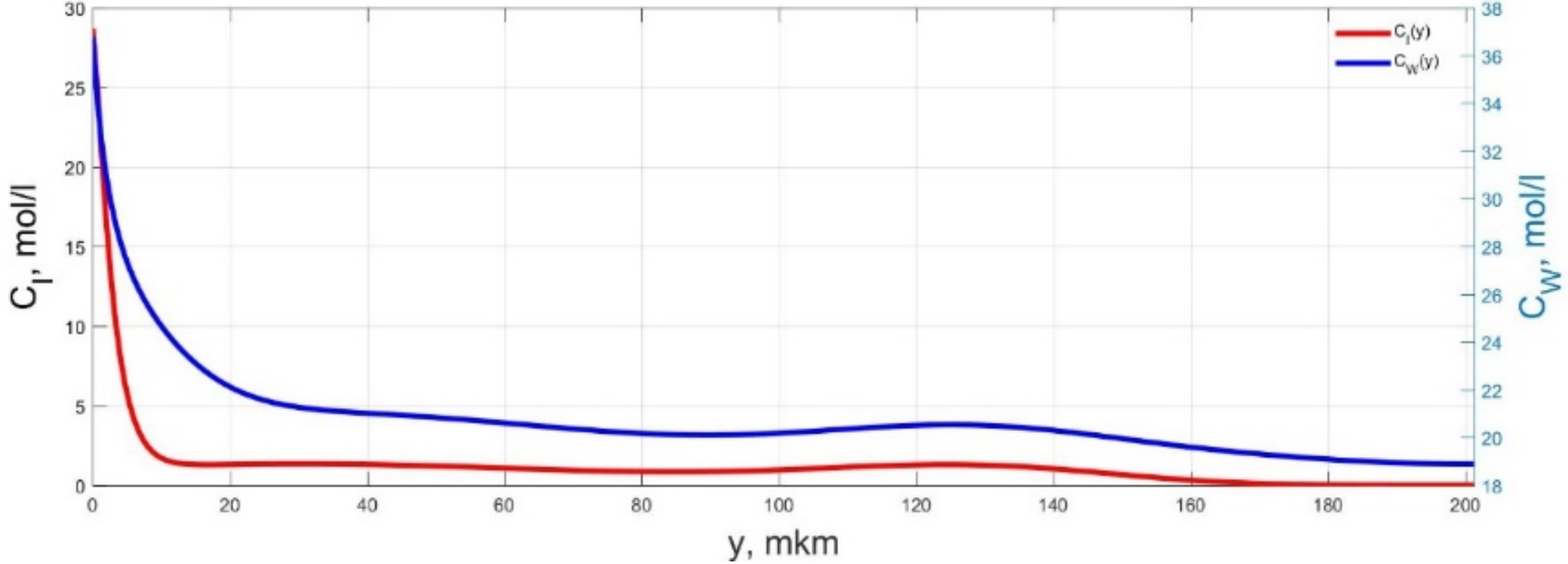
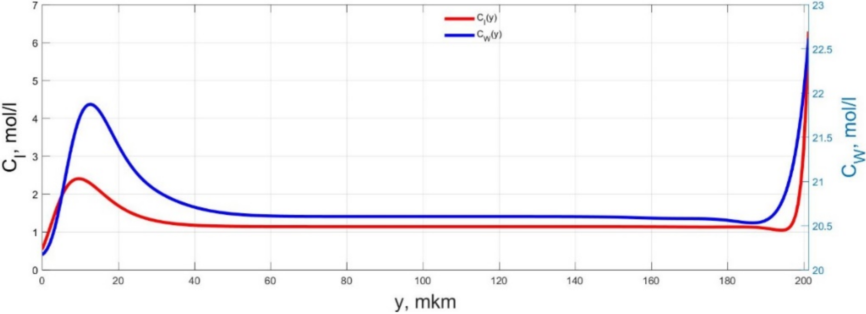
- Subsystem 2 (7)–(14)where is the grid function of the concentration of water molecules.
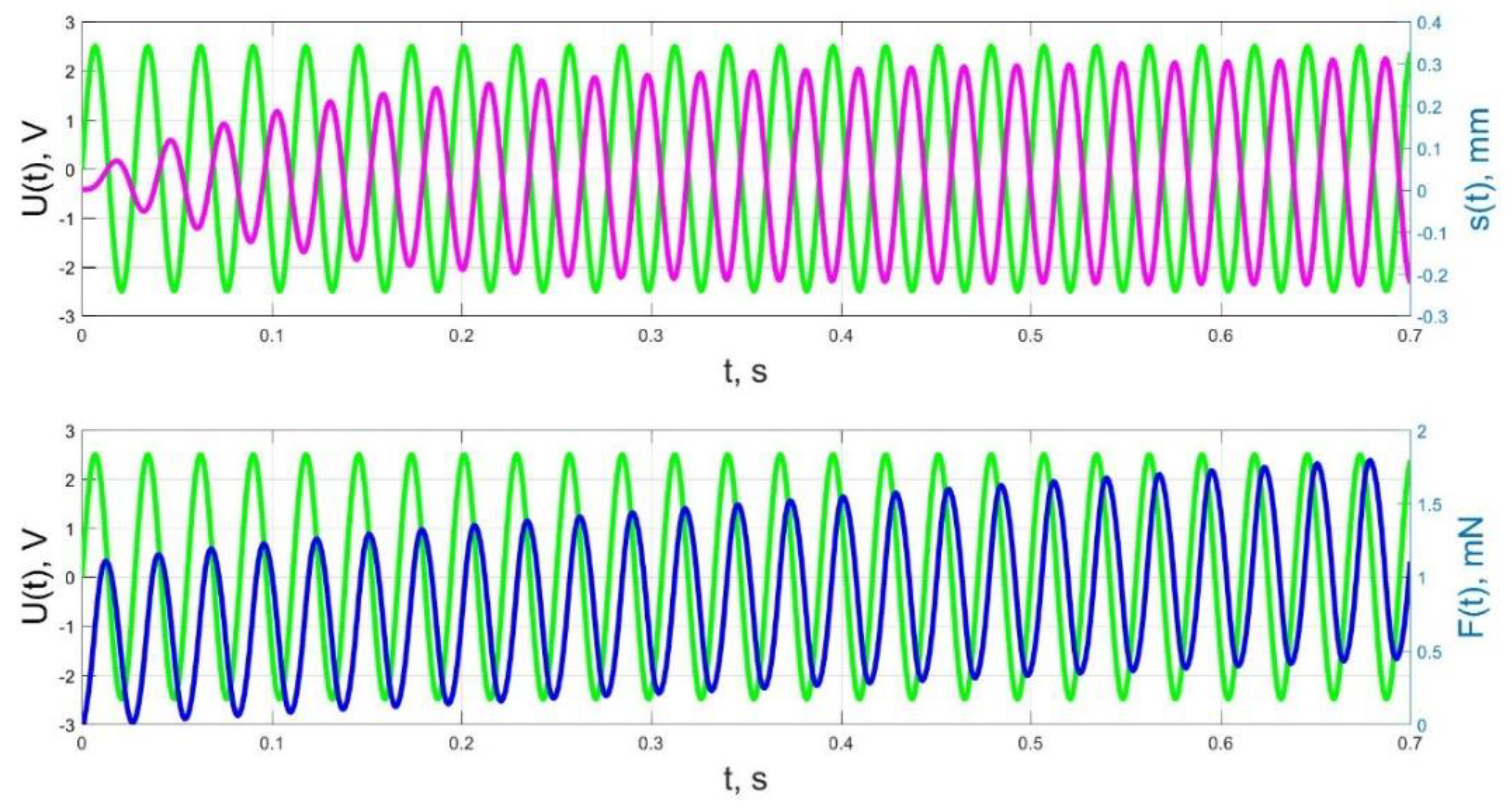
- Subsystem 3 (26)–(28) was discretized on the time grid (32) and the extended non-uniform coordinate gridincluding the coordinate grid (33), supplemented by the first and last nodes, the coordinates of which correspond to the outer boundaries of metal electrodeswhere is the grid function of the tip displacement of the cantilever beam; is the grid function of the Young’s modulus; is the grid function of the resonant frequency; is the grid function of the linear density of the beam.
4. Model Verification, Results, and Discussion
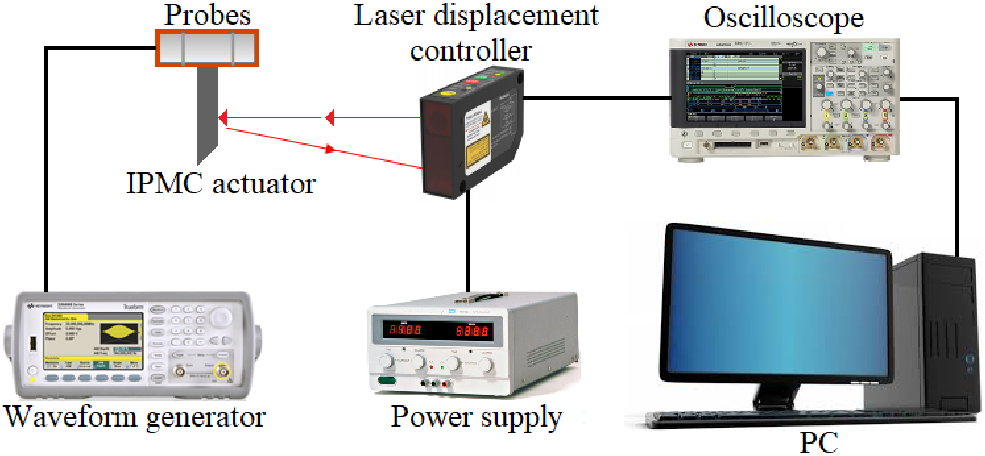
4.1. Experimental Setup
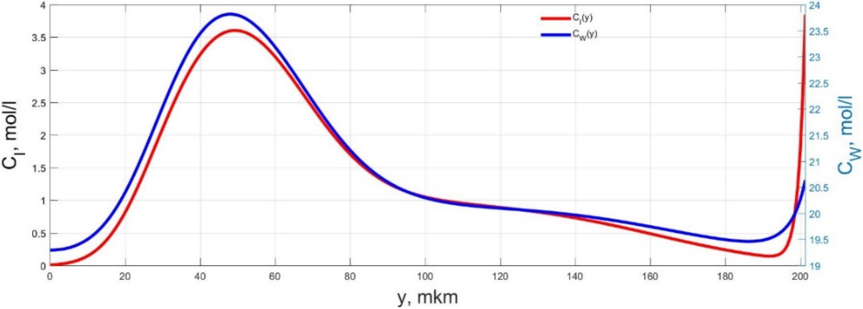
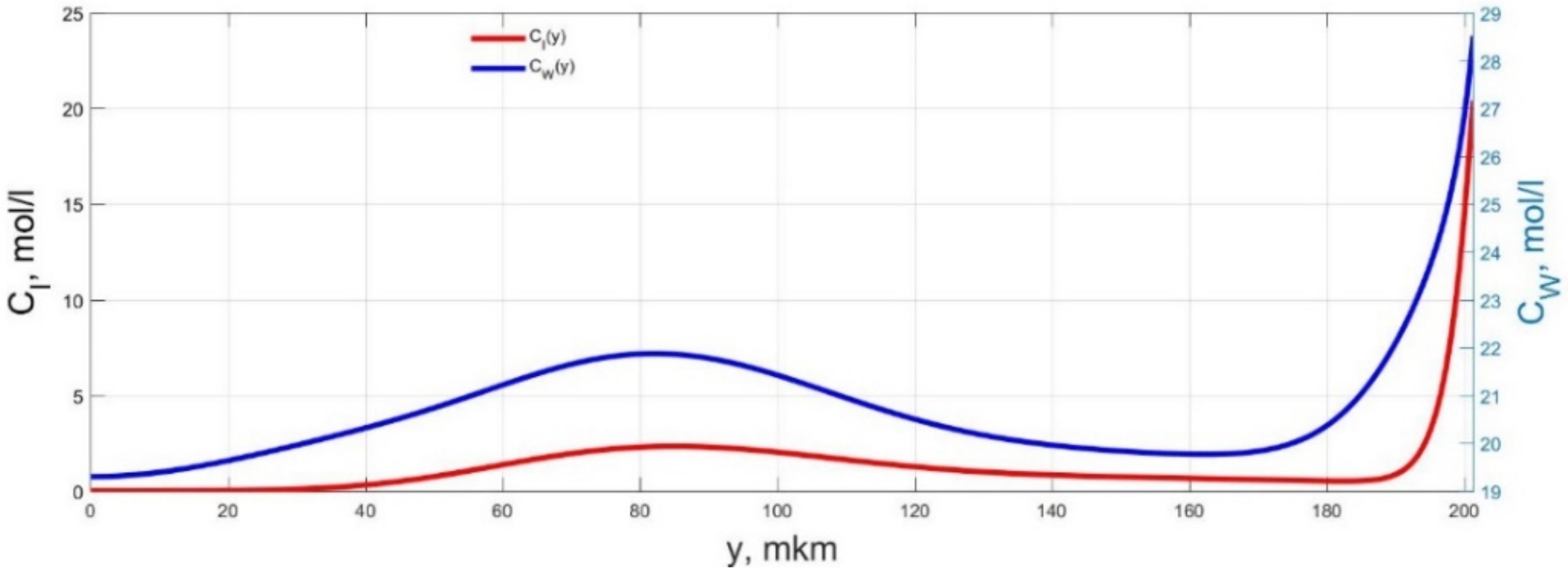
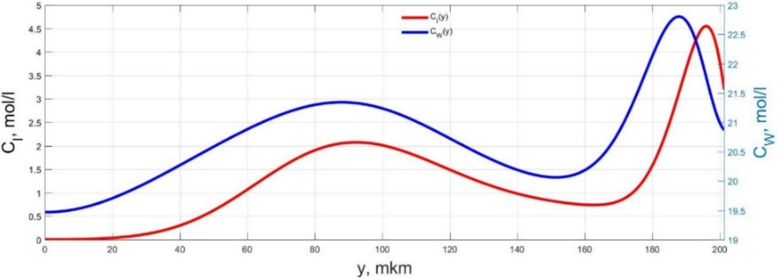
4.2. Numerical Simulation Results and Their Discussion—Comparison with Experimental Data
5. Conclusions
Author Contributions
Funding
Conflicts of Interest
References
- Takagi, K.; Shahinpoor, M.; Schneider, H.-J.; Oh, I.-K.; Porfiri, M.; Kim, K.J.; Johanson, U.; Vunder, V.; Branco, P.J.C.; Tan, X.; et al. Ionic Polymer Metal. Composites (IPMCs): Smart Multi-Functional Materials and Artificial Muscles, 1st ed.; Shahinpoor, M., Ed.; Royal Society of Chemistry: Cambridge, UK, 2015; Volume 1, ISBN 978-1-78262-258-1. [Google Scholar]
- Kalyonov, V.E.; Orekhov, Y.D.; Khmelnitskiy, I.K.; Alekseev, N.I.; Broyko, A.P.; Lagosh, A.V.; Testov, D.O.; Shpakovsky, A.D. Walking Robot with Propulsors Based on IPMC Actuators. In Proceedings of the 2019 IEEE International Conference on Electrical Engineering and Photonics (EExPolytech), St. Petersburg, Russia, 17–18 October 2019; pp. 169–172. [Google Scholar] [CrossRef]
- Yu, M.; Shen, H.; Dai, Z.-D. Manufacture and Performance of Ionic Polymer-Metal Composites. J. Bionic Eng. 2007, 4, 143–149. [Google Scholar] [CrossRef]
- Alekseev, N.I.; Bagrets, V.V.; Broyko, A.P.; Korlyakov, A.V.; Kalenov, V.E.; Luchinin, V.V.; Sevostyanov, E.N.; Testov, D.O.; Khmelnitsky, I.K. Ionic Polymer Electroactive Actuators Based on the MF-4SK Ion-Exchange Membrane. Part 1. Ionic Polymer-Metal Composites. J. Struct. Chem. 2020, 61, 601–608. [Google Scholar] [CrossRef]
- Lagosh, A.V.; Broyko, A.P.; Kalyonov, V.E.; Khmelnitskiy, I.K.; Luchinin, V.V. Modeling of IPMC Actuator. In Proceedings of the 2017 IEEE Conference of Russian Young Researchers in Electrical and Electronic Engineering (EIConRus), St. Petersburg, Russia, 1–3 February 2017; pp. 916–918. [Google Scholar] [CrossRef]
- Shahinpoor, M.; Kim, K.J. Ionic polymer-metal composites: III. Modeling and simulation as biomimetic sensors, actuators, transducers, and artificial muscles. Smart Mater. Struct. 2004, 13, 1362–1388. [Google Scholar] [CrossRef]
- Kalyonov, V.E.; Lagosh, A.V.; Khmelnitskiy, I.K.; Broyko, A.P.; Korlyakov, A.V. The Electromechanical Model of Ionic Polymer-Metal Composite Actuator. In Proceedings of the 2017 IEEE Conference of Russian Young Researchers in Electrical and Electronic Engineering (EIConRus), St. Petersburg, Russia, 1–3 February 2017; pp. 883–886. [Google Scholar] [CrossRef]
- Zakeri, E.; Moeinkhah, H. Digital control design for an IPMC actuator using adaptive optimal proportional integral plus method: Simulation and experimental study. Sens. Actuators A 2019, 298, 111577. [Google Scholar] [CrossRef]
- Park, K.; Lee, H.-K. Evaluation of Circuit Models for an IPMC (Ionic Polymer-Metal Composite) Sensor Using a Parameter Estimate Method. J. Korean Phys. Soc. 2012, 60, 821–829. [Google Scholar] [CrossRef]
- Nemat-Nasser, S. Micromechanics of actuation of ionic polymer-metal composites. J. Appl. Phys. 2002, 92, 2899–2915. [Google Scholar] [CrossRef] [Green Version]
- Xiao, Y.; Bhattacharya, K. Modeling electromechanical properties of ionic polymers. Proc. SPIE 2001, 4329, 292–300. [Google Scholar] [CrossRef]
- Bass, P.S.; Zhang, L.; Cheng, Z.-Y. Time-dependence of the electromechanical bending actuation observed in ionic-electroactive polymers. J. Adv. Dielectr. 2017, 7, 1720002. [Google Scholar] [CrossRef] [Green Version]
- Bass, P.S.; Zhang, L.; Tu, M.; Cheng, Z.Y. Enhancement of Biodegradable Poly (Ethylene Oxide) Ionic–Polymer Metallic Composite Actuators with Nanocrystalline Cellulose Fillers. Actuators 2018, 7, 72. [Google Scholar] [CrossRef] [Green Version]
- Ji, A.-H.; Park, H.C.; Nguyen, Q.V.; Lee, J.W.; Yoo, Y.T. Verification of Beam Models for Ionic Polymer-Metal Composite Actuator. J. Bionic Eng. 2009, 6, 232–238. [Google Scholar] [CrossRef]
- Zhu, Z.; Chen, H.; Chang, L.; Li, B. Dynamic model of ion and water transport in ionic polymer-metal composites. AIP Adv. 2011, 1, 040702. [Google Scholar] [CrossRef]
- Kondo, K.; Takagi, K.; Zhu, Z.; Asaka, K. Symbolic finite element discretization and model order reduction of a multiphysics model for IPMC sensors. Smart Mater. Struct. 2020, 29, 115037. [Google Scholar] [CrossRef]
- Zhu, Z.; Chen, H.; Wang, Y. Sensing Properties and Physical Model of Ionic Polymer. In Soft Actuators, 2nd ed.; Asaka, K., Okuzaki, H., Eds.; Springer: Singapore, 2019; pp. 503–545. ISBN 978-981-13-6850-9. [Google Scholar]
- Timoshenko, S.P.; Young, D.H.; Weaver, W. Vibration Problems in Engineering, 4th ed.; John Wiley & Sons: New York, NY, USA, 1974; ISBN 978-1406774658. [Google Scholar]
- Donnell, L.H. Beams, Plates and Shells, 1st ed.; McGraw-Hill: New York, NY, USA, 1976; ISBN 978-0070175938. [Google Scholar]
- Caponetto, R.; De Luca, V.; Di Pasquale, G.; Graziani, S.; Sapuppo, F.; Umana, E. A new multi-physics model of an IP2C actuator in the electrical, chemical, mechanical and thermal domains. In Proceedings of the 2013 IEEE International Instrumentation and Measurement Technology Conference (I2MTC), Minneapolis, MN, USA, 6–9 May 2013; pp. 971–975. [Google Scholar]
- Kalyonov, V.E.; Alekseev, N.I.; Khmelnitskiy, I.K.; Lagosh, A.V.; Broyko, A.P. Free Oscillation Frequency of IPMC Actuator as an Indicator of its Water Content. In Proceedings of the 2019 IEEE Conference of Russian Young Researchers in Electrical and Electronic Engineering (EIConRus), St. Petersburg/Moscow, Russia, 28–31 January 2019; pp. 812–814. [Google Scholar] [CrossRef]
- Khmelnitskiy, I.K.; Vereschagina, L.O.; Kalyonov, V.E.; Lagosh, A.V.; Broyko, A.P. Improvement of Manufacture Technology and Investigation of IPMC Actuator Electrodes. In Proceedings of the 2017 IEEE Conference of Russian Young Researchers in Electrical and Electronic Engineering (EIConRus), St. Petersburg, Russia, 1–3 February 2017; pp. 892–895. [Google Scholar] [CrossRef]
- Khmelnitskiy, I.K.; Vereshagina, L.O.; Kalyonov, V.E.; Broyko, A.P.; Lagosh, A.V.; Luchinin, V.V.; Testov, D.O. Improvement of manufacture technology and research of actuators based on ionic polymer-metal composites. J. Phys. Conf. Ser. 2017, 857, 12018. [Google Scholar] [CrossRef]


| Parameter | Symbol | Value | Unit |
|---|---|---|---|
| Polymer trademark | – | Nafion N117 | – |
| Length of the dry beam 1 | L | 15 | mm |
| Width of the dry beam 1 | w | 5 | mm |
| Thickness of the dry beam 1 | H | 183 | μm |
| Thickness of metal electrodes | H | 5 | μm |
| Temperature | T | 293 | K |
| Diffusion coefficient of cations | DII | 5.3 × 10⁻⁶ | cm2⋅s−1 |
| Diffusion coefficient of water molecules | DWW | 3.87 × 10⁻⁶ | cm2⋅s−1 |
| Concentration of ions in the polymer | C + | 0.9 | mol⋅kg−1 |
| Molar volume of ions | VI | −5.4 | cm3⋅mol−1 |
| Molar volume of water | VW | 18 | cm3⋅mol−1 |
| Filtration coefficient | K | 3.4 × 10⁻¹⁴ | cm2⋅Pa−1⋅s−1 |
| Elementary charge | q | 1.6 × 10⁻¹⁹ | C |
| Faraday constant | F | 96,485 | C⋅mol−1 |
| Gas constant | R | 8.31 | J⋅K−1⋅mol−1 |
| Permittivity of vacuum | ε0 | 8.85 × 10⁻¹⁴ | F⋅cm−1 |
| Relative permittivity of water | ε | 81 | – |
| Expansion coefficient of the membrane at maximum humidification | α | 0.1 | – |
| Relative charge of ion | ZI | 1 | – |
| Number of water molecules associated with one cation | ndW | 1 | – |
| Mass fraction of water in the dry polymer 1 | PWN | 0.05 | – |
| Mass fraction of water in the humidified polymer | PWS | 0.38 | – |
| Young’s modulus of the dry polymer 1 | EN | 249 | MPa |
| Young’s modulus of the humidified polymer | ES | 114 | MPa |
| Young’s modulus of metal electrodes | EM | 23 | GPa |
| Empirical coefficient | ηI | 200 | MPa |
| Empirical coefficient | ηW | 200 | MPa |
| Coefficient depending on the mode of beam bending oscillations | λ | 3.52 | – |
| Coefficient characterizing dissipative processes | β | 19 | s−1 |
| Empirical coefficient determining the evaporation rate of cations into the external environment | γI | 0 | – |
| Empirical coefficient determining the evaporation rate of water molecules into the external environment | γW | 0 | – |
| Layer density of the dry membrane 1 | ρSPN | 3.6 × 10⁻² | g·cm−2 |
| Density of the electrode material | ρM | 21.5 | g·cm−3 |
| Molar mass of water | MW | 18.01528 | g⋅mol−1 |
Publisher’s Note: MDPI stays neutral with regard to jurisdictional claims in published maps and institutional affiliations. |
© 2020 by the authors. Licensee MDPI, Basel, Switzerland. This article is an open access article distributed under the terms and conditions of the Creative Commons Attribution (CC BY) license (http://creativecommons.org/licenses/by/4.0/).
Share and Cite
Broyko, A.P.; Khmelnitskiy, I.K.; Ryndin, E.A.; Korlyakov, A.V.; Alekseyev, N.I.; Aivazyan, V.M. Multiphysics Simulator for the IPMC Actuator: Mathematical Model, Finite Difference Scheme, Fast Numerical Algorithm, and Verification. Micromachines 2020, 11, 1119. https://doi.org/10.3390/mi11121119
Broyko AP, Khmelnitskiy IK, Ryndin EA, Korlyakov AV, Alekseyev NI, Aivazyan VM. Multiphysics Simulator for the IPMC Actuator: Mathematical Model, Finite Difference Scheme, Fast Numerical Algorithm, and Verification. Micromachines. 2020; 11(12):1119. https://doi.org/10.3390/mi11121119
Chicago/Turabian StyleBroyko, Anton P., Ivan K. Khmelnitskiy, Eugeny A. Ryndin, Andrey V. Korlyakov, Nikolay I. Alekseyev, and Vagarshak M. Aivazyan. 2020. "Multiphysics Simulator for the IPMC Actuator: Mathematical Model, Finite Difference Scheme, Fast Numerical Algorithm, and Verification" Micromachines 11, no. 12: 1119. https://doi.org/10.3390/mi11121119