
Scale Effects of the Relationships between Urban Heat Islands and Impact Factors Based on a Geographically-Weighted Regression Model

Abstract
:
1. Introduction
2. Study Area
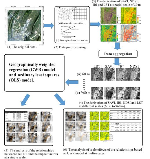
3. Methods
3.1. Image Pre-Processing
3.2. Derivation of the Parameters and Data Aggregation
3.2.1. Dependent Variable: LST
3.2.2. Explanatory Variables: SAVI, IBI, and NDSI
3.2.3. Data aggregation
3.3. Geographically-Weighted Regression
4. Results
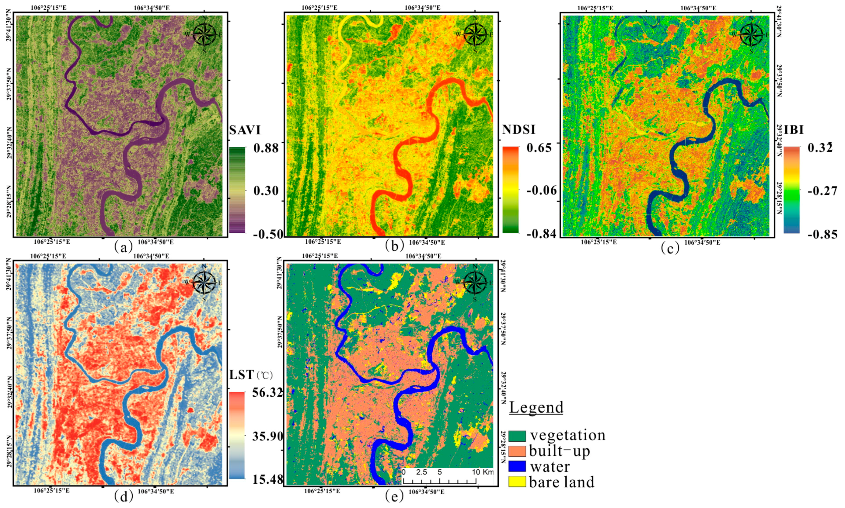
4.1. The Derivation Results of SAVI, IBI, NDSI, LST and Classification Result of the Study Area
4.2. Data Sampling
4.3. The Analysis of the Relationships between the LST and the Impact Factors at a Single Scale
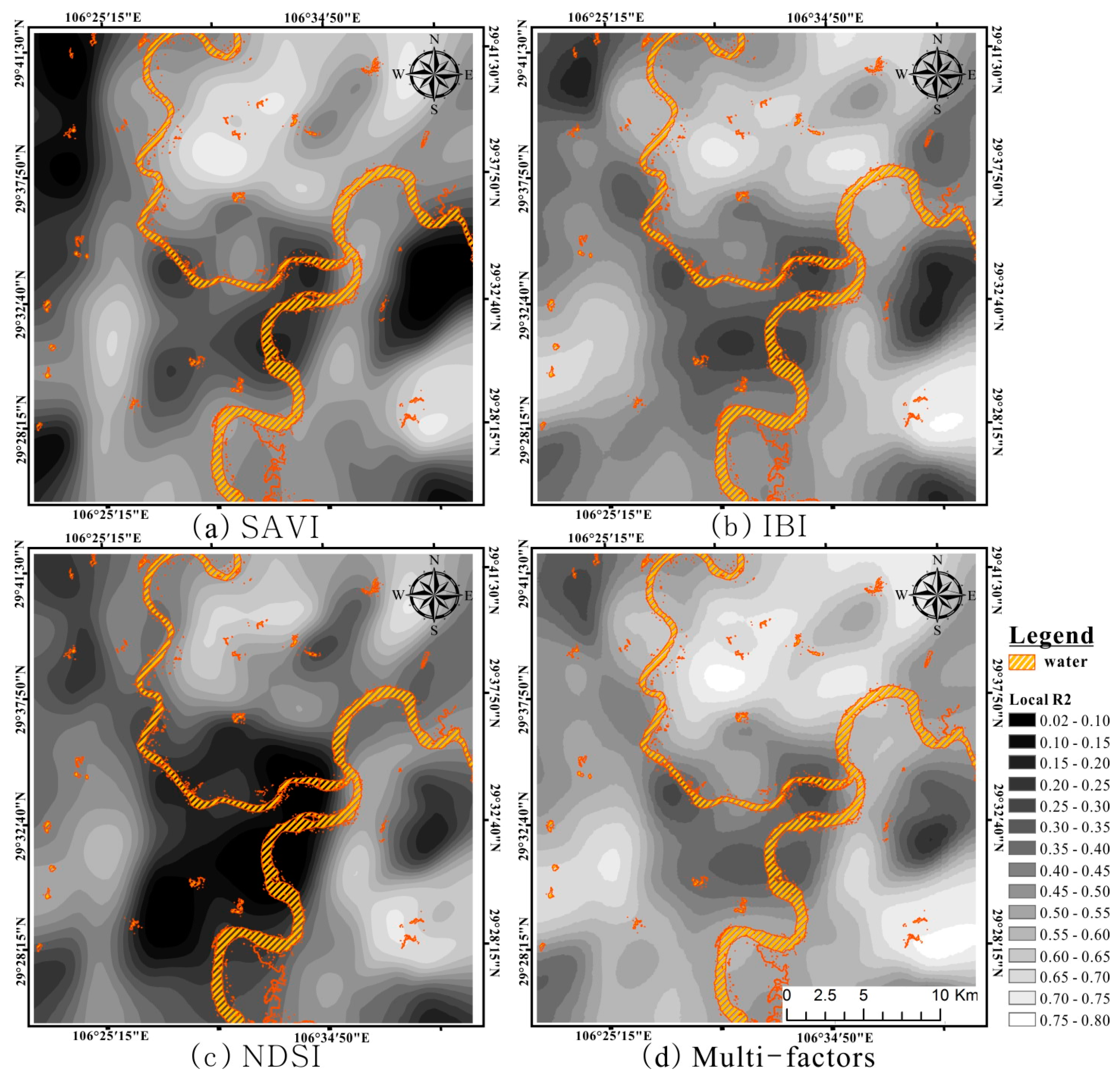
4.3.1. Comparisons between the OLS and GWR Models
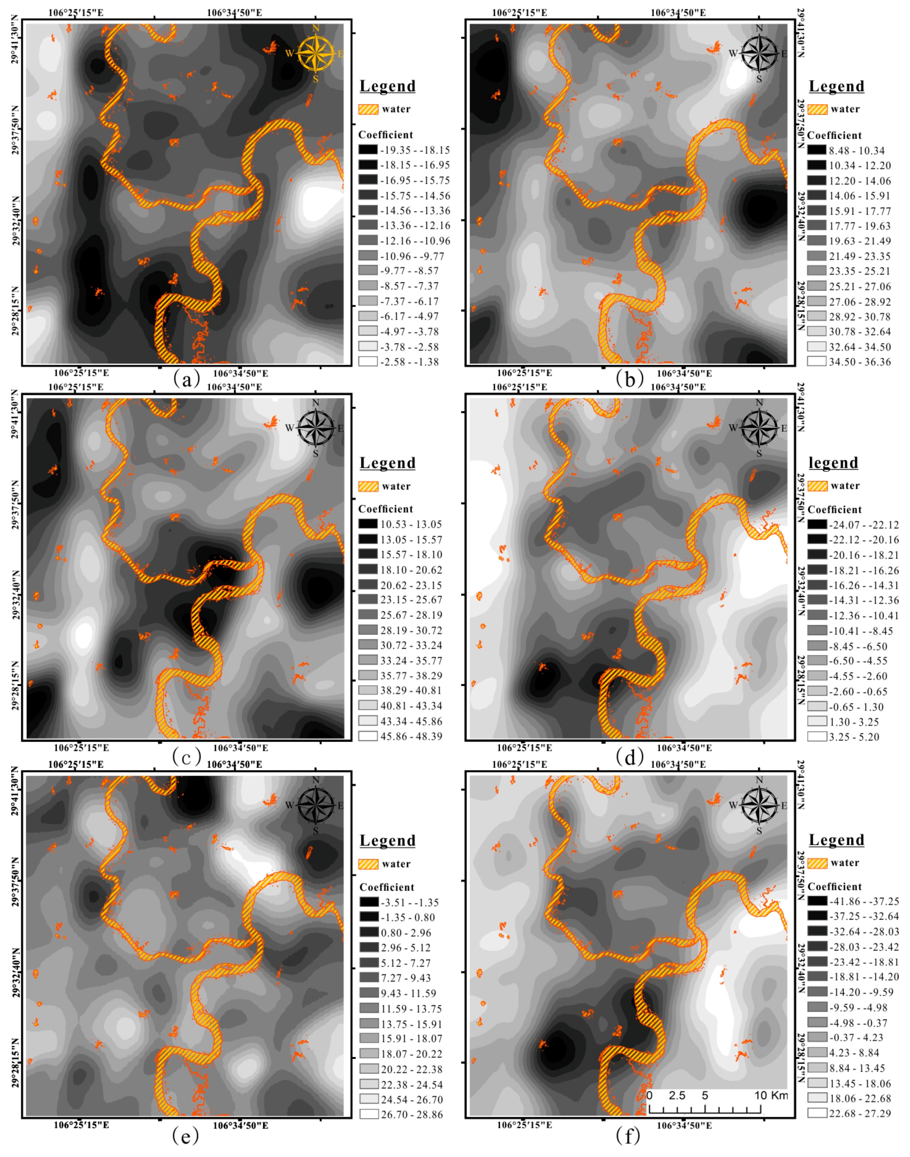
4.3.2. Spatial Non-Stationarity among Relationships
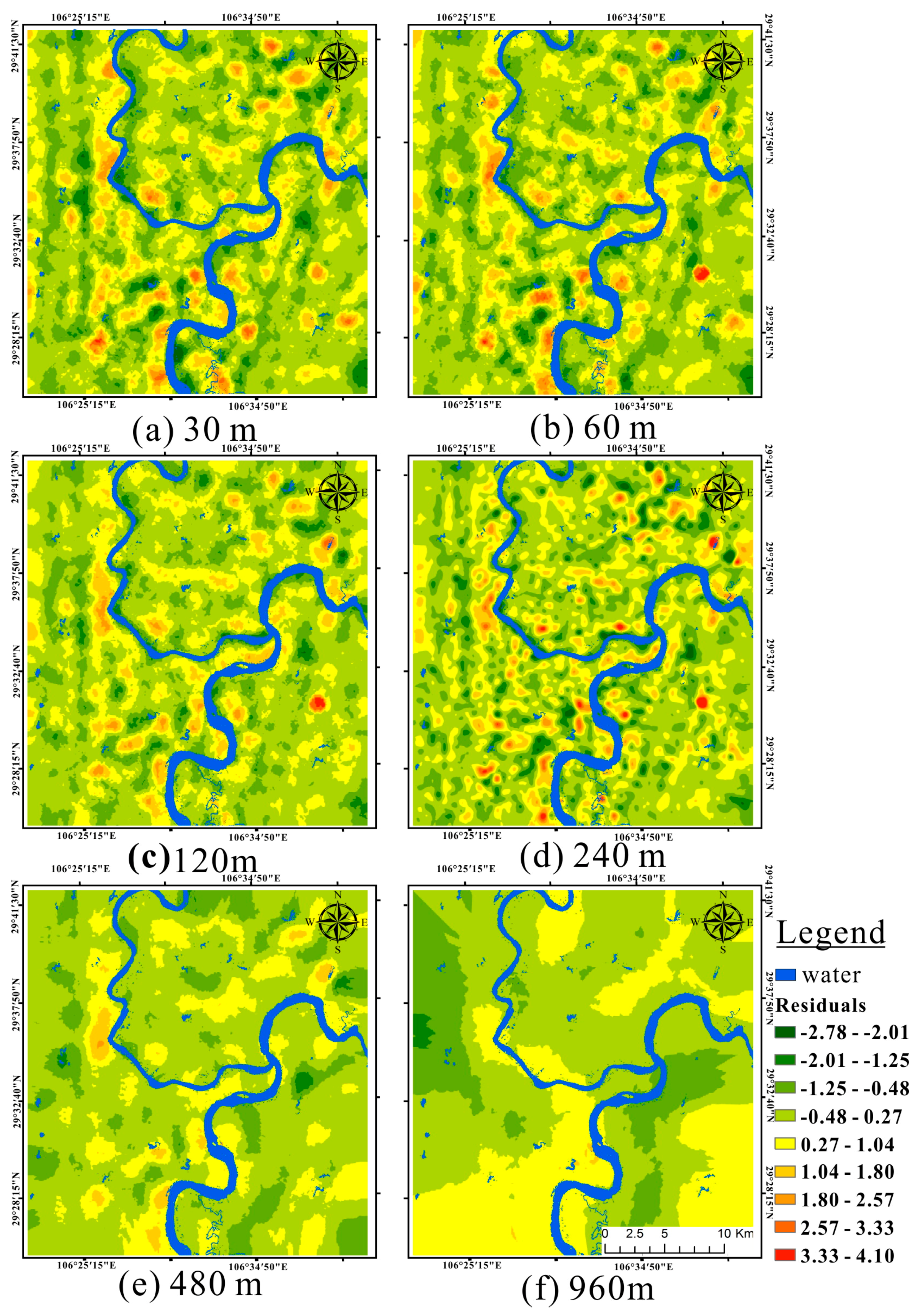
4.4. Scale Effects of the Relationships Based on the GWR model at Multiple Scales
5. Discussion
6. Conclusions
- Both single-factor and multi-factors GWR models have better prediction accuracies, characterized by much smaller AICc values, higher adjusted R2 values, and better F-tests, when compared with the corresponding OLS models. At the same time, both the coefficients and the local R2 of the GWR models are changing with the spatial location, and this indicates that the GWR has a good ability to characterize the non-stationarity of the relationships between the LST and the indices.
- With the increase of spatial scales, the overall fitting degree of the GWR model is gradually improved based on the distribution range, the mean value of local R2. However, the standard deviation of the local R2 and residuals are gradually reduced from 0.22 (30 m) to 0.03 (960 m) and 1.83 (30 m) to 0.52 (960 m), respectively. Meanwhile, the Moran’s I values of the residuals gradually increase from 0.19 (30 m) to 0.39 (960 m). This indicates the GWR model becomes increasingly global, revealing the relationships with more generalized geographical patterns, and then spatial non-stationarity in the relationship tends to be neglected with the increase of the spatial resolution.
- Characterized by higher R2 value and lower AICc value, GWR models have better ability than OLS models to explain the relationships between SUHI and impact factors (the SAVI, IBI, and NDSI) at small spatial scales (30 m–240 m), and when the spatial scale is increased to 480 m and 960 m, this advantage has become relatively weak because the GWR model becomes increasingly global, revealing the relationships with more generalized geographical patterns, and then spatial non-stationarity in the relationship tends to be neglected with the increase of the spatial resolution. Therefore, if the spatial resolution of remote sensing data is less than 240 m, GWR mode is recommended to be used in the monitoring and analysis of SUHI in the mountain city, and when the spatial resolution is greater than 480 m, both GWR and OLS models are suitable for the researches of SUHI because there are few performance differences between them.
Acknowledgments
Author Contributions
Conflicts of Interest
Abbreviations
| GWR | Geographically weighted regression |
| OLS | Ordinary least squares |
| UHI | Urban heat island |
| LST | Land surface temperature |
| SAVI | Soil-adjusted Vegetation Index |
| IBI | Index-based Built-up Index |
| NDSI | Soil Brightness Index |
| NDVI | Normalized Difference Vegetation Index |
| NDWI | Normalized Difference Water Index |
| NDBI | Normalized Difference Built-up Index |
| NDBaI | Normalized Difference Bareness Index |
| ANN | Artificial neural network |
| TM | Thematic Mapper |
| TOA | Top-of-atmospheric radiance |
| AICc | Corrected Akaike Information Criterion |
| R2 | Coefficient of determination |
| Moran’s I | Moran’s Index |
References
- Oke, T. Urban climates and global environmental change. In Applied Climatology: Principles & Practices; Thompson, R.D., Perry, A.H., Eds.; Routledge: New York, NY, USA, 1997; pp. 273–287. [Google Scholar]
- Voogt, J.A. Urban heat island. In Encyclopedia of Global Environmental Change; Munn, T., Ed.; John Wiley & Sons Ltd.: Chichester, UK, 2002; pp. 660–666. [Google Scholar]
- Mirzaei, P.A. Recent challenges in modeling of urban heat island. Sustain. Cities Soc. 2015, 19, 200–206. [Google Scholar] [CrossRef]
- Price, J.C. Land surface temperature measurements from the split window channels of the noaa 7 advanced very high resolution radiometer. J. Geophys. Res. Atmos. 1984, 89, 7231–7237. [Google Scholar] [CrossRef]
- Carlson, T.N.; Arthur, S.T. The impact of land use—Land cover changes due to urbanization on surface microclimate and hydrology: A satellite perspective. Glob. Planet. Chang. 2000, 25, 49–65. [Google Scholar] [CrossRef]
- Streutker, D.R. A remote sensing study of the urban heat island of Houston, Texas. Int. J. Remote Sens. 2002, 23, 2595–2608. [Google Scholar] [CrossRef]
- Streutker, D.R. Satellite-measured growth of the urban heat island of Houston, Texas. Remote Sens. Environ. 2003, 85, 282–289. [Google Scholar] [CrossRef]
- Weng, Q.; Lu, D.; Schubring, J. Estimation of land surface temperature–vegetation abundance relationship for urban heat island studies. Remote Sens. Environ. 2004, 89, 467–483. [Google Scholar] [CrossRef]
- Yuan, F.; Bauer, M.E. Comparison of impervious surface area and normalized difference vegetation index as indicators of surface urban heat island effects in landsat imagery. Remote Sens. Environ. 2007, 106, 375–386. [Google Scholar] [CrossRef]
- Weng, Q.; Rajasekar, U.; Hu, X. Modeling urban heat islands and their relationship with impervious surface and vegetation abundance by using aster images. IEEE Trans. Geosci. Remote Sens. 2011, 49, 4080–4089. [Google Scholar] [CrossRef]
- Jusuf, S.K.; Wong, N.H.; Hagen, E.; Anggoro, R.; Yan, H. The influence of land use on the urban heat island in singapore. Habitat Int. 2007, 31, 232–242. [Google Scholar] [CrossRef]
- Callejas, A.I.J.; de Oliveira, A.S.; de Moura Santos, F.M.; Durante, L.C.; de Jesus Albuquerque Nogueira, M.C.; Zeilhofer, P. Relationship between land use/cover and surface temperatures in the urban agglomeration of cuiabá-várzea grande, central Brazil. J. Appl. Remote Sens. 2011, 5, 053569. [Google Scholar] [CrossRef]
- Imhoff, M.L.; Zhang, P.; Wolfe, R.E.; Bounoua, L. Remote sensing of the urban heat island effect across biomes in the continental USA. Remote Sens. Environ. 2010, 114, 504–513. [Google Scholar] [CrossRef]
- Chen, X.L.; Zhao, H.M.; Li, P.X.; Yin, Z.Y. Remote sensing image-based analysis of the relationship between urban heat island and land use/cover changes. Remote Sens. Environ. 2006, 104, 133–146. [Google Scholar] [CrossRef]
- Ogashawara, I.; Bastos, V.S.B. A quantitative approach for analyzing the relationship between urban heat islands and land cover. Remote Sens. 2012, 4, 3596–3618. [Google Scholar] [CrossRef]
- Luo, X.; Li, W. Scale effect analysis of the relationships between urban heat island and impact factors: Case study in chongqing. J. Appl. Remote Sens. 2014, 8, 284–292. [Google Scholar] [CrossRef]
- Ashtiani, A.; Mirzaei, P.A.; Haghighat, F. Indoor thermal condition in urban heat island: Comparison of the artificial neural network and regression methods prediction. Energy Build. 2014, 76, 597–604. [Google Scholar] [CrossRef]
- Mirzaei, P.A.; Olsthoorn, D.; Torjan, M.; Haghighat, F. Urban neighborhood characteristics influence on a building indoor environment. Sustain. Cities Soc. 2015, 19, 403–413. [Google Scholar] [CrossRef]
- Lee, Y.Y.; Kim, J.T.; Yun, G.Y. The neural network predictive model for heat island intensity in seoul. Energy Build. 2016, 110, 353–361. [Google Scholar] [CrossRef]
- Brunsdon, C.; Fotheringham, A.S.; Charlton, M.E. Geographically weighted regression: A method for exploring spatial nonstationarity. Geogr. Anal. 1996, 28, 281–298. [Google Scholar] [CrossRef]
- Brown, S.; Versace, V.L.; Laurenson, L.; Ierodiaconou, D.; Fawcett, J.; Salzman, S. Assessment of spatiotemporal varying relationships between rainfall, land cover and surface water area using geographically weighted regression. Environ. Model. Assess. 2012, 17, 241–254. [Google Scholar] [CrossRef]
- Fotheringham, A.S.; Brunsdon, C.; Charlton, M. Geographically Weighted Regression—The Analysis of Spatially Varying Relationships; John Wiley & Sons Ltd.: WestSussex, UK, 2002. [Google Scholar]
- Brunsdon, C.; Mcclatchey, J.; Unwin, D.J. Spatial variations in the average rainfall–altitude relationship in great britain: An approach using geographically weighted regression. Int. J. Climatol. 2001, 21, 455–466. [Google Scholar] [CrossRef]
- Foody, G.M. Geographical weighting as a further refinement to regression modelling: An example focused on the ndvi–rainfall relationship. Remote Sens. Environ. 2003, 88, 283–293. [Google Scholar] [CrossRef]
- Longley, P.A.; Tobón, C. Spatial dependence and heterogeneity in patterns of hardship: An intra-urban analysis. Ann. Assoc. Am. Geogr. 2004, 94, 503–519. [Google Scholar] [CrossRef]
- Zhang, C.S.; Tang, Y.; Lin, L.; Xu, W.L. Outlier identification and visualization for pb concentrations in urban soils and its implications for identification of potential contaminated land. Environ. Pollut. 2009, 157, 3083–3090. [Google Scholar] [CrossRef] [PubMed]
- Mennis, J.L.; Jordan, L. The distribution of environmental equity: Exploring spatial nonstationarity in multivariate models of air toxic releases. Ann. Assoc. Am. Geogr. 2005, 95, 249–268. [Google Scholar] [CrossRef]
- Tu, J.; Xia, Z.G. Examining spatially varying relationships between land use and water quality using geographically weighted regression I: Model design and evaluation. Sci. Total Environ. 2008, 407, 358–378. [Google Scholar] [CrossRef] [PubMed]
- Gao, J.; Li, S. Detecting spatially non-stationary and scale-dependent relationships between urban landscape fragmentation and related factors using geographically weighted regression. Appl. Geogr. 2011, 31, 292–302. [Google Scholar] [CrossRef]
- Javi, S.T.; Malekmohammadi, B.; Mokhtari, H. Application of geographically weighted regression model to analysis of spatiotemporal varying relationships between groundwater quantity and land use changes (case study: Khanmirza Plain, Iran). Environ. Monit. Assess. 2014, 186, 3123–3138. [Google Scholar] [CrossRef] [PubMed]
- Zhao, Z.; Gao, J.; Wang, Y.; Liu, J.; Li, S. Exploring spatially variable relationships between ndvi and climatic factors in a transition zone using geographically weighted regression. Theor. Appl. Climatol. 2015, 120, 507–519. [Google Scholar] [CrossRef]
- Li, S.; Zhao, Z.; Miaomiao, X.; Wang, Y. Investigating spatial non-stationary and scale-dependent relationships between urban surface temperature and environmental factors using geographically weighted regression. Environ. Model. Softw. 2010, 25, 1789–1800. [Google Scholar] [CrossRef]
- Buyantuyev, A.; Wu, J. Urban heat islands and landscape heterogeneity: Linking spatiotemporal variation in surface temperatures to land-cover and socioeconomic patterns. Landsc. Ecol. 2010, 25, 17–33. [Google Scholar] [CrossRef]
- Su, Y.F.; Foody, G.M.; Cheng, K.S. Spatial non-stationarity in the relationships between land cover and surface temperature in an urban heat island and its impacts on thermally sensitive populations. Landsc. Urban Plan. 2012, 107, 172–180. [Google Scholar] [CrossRef]
- Tian, F.; Qiu, G.Y.; Yang, Y.H.; Xiong, Y.J. Studies on the relationships between land surface temperature and environmental factors in an inland river catchment based on geographically weighted regression and modis data. IEEE J. Sel. Top. Appl. Earth Obs. Remote Sens. 2012, 5, 687–698. [Google Scholar] [CrossRef]
- Huete, A.R. A soil-adjusted vegetation index (savi). Remote Sens. Environ. 1988, 25, 295–309. [Google Scholar] [CrossRef]
- Xu, H. A new index for delineating built-up land features in satellite imagery. Int. J. Remote Sens. 2008, 29, 4269–4276. [Google Scholar] [CrossRef]
- Xu, J.C.; Zhao, Y.S.; Liu, Z.H. Research on ecological environment change of middle and western inner-mongolia region using RS and GIS. J. Remote Sens. 2002, 6, 142–149. [Google Scholar]
- Chander, G.; Markham, B. Revised landsat-5 tm radiometric calibration procedures and postcalibration dynamic ranges. IEEE Trans. Geosci. Remote Sens. 2003, 41, 2674–2677. [Google Scholar] [CrossRef]
- Barsi, J.A.; Schott, J.R.; Palluconi, F.D.; Hook, S.J. Validation of a web-based atmospheric correction tool for single thermal band instruments. In Proceedings of SPIE-The International Society for Optical Engineering, San Diego, CA, USA, 31 July–2 August 2005; pp. 58820E–58827.
- Atmospheric Correction Parameter Calculator. Available online: http://atmcorr.gsfc.nasa.gov/ (accessed on 12 September 2016).
- Qin, Z.H.; Wen juan, L.I.; Bin, X.U.; Chen, Z.X.; Liu, J. The estimation of land surface emissivity for landsat TM6. Remote Sens. Land Resour. 2004, 3, 28–32. [Google Scholar]
- Shi, H.; Laurent, E.J.; Lebouton, J.; Racevskis, L.; Hall, K.R.; Donovan, M.; Doepker, R.V.; Walters, M.B.; Lupi, F.; Liu, J. Local spatial modeling of white-tailed deer distribution. Ecol. Model. 2006, 190, 171–189. [Google Scholar] [CrossRef]
- Hurvich, C.M.; Simonoff, J.S.; Tsai, C.L. Smoothing parameter selection in nonparametric regression using an improved akaike information criterion. J. R. Stat. Soc. 1998, 60, 271–293. [Google Scholar] [CrossRef]
- Propastin, P.A. Spatial non-stationarity and scale-dependency of prediction accuracy in the remote estimation of lai over a tropical rainforest in sulawesi, indonesia. Remote Sens. Environ. 2009, 113, 2234–2242. [Google Scholar] [CrossRef]
- Cui, L.; Shi, J.; Yang, Y.; Fan, W. Ten-day response of vegetation ndvi to the variations of temperature and precipitation in Eastern China. Acta Geogr. Sin. 2009, 7, 011. [Google Scholar]
- Finley, A.O. Comparing spatially-varying coefficients models for analysis of ecological data with non-stationary and anisotropic residual dependence. Methods Ecol. Evol. 2011, 2, 143–154. [Google Scholar] [CrossRef]
- Yu, D.-L. Spatially varying development mechanisms in the greater Beijing area: A geographically weighted regression investigation. Ann. Reg. Sci. 2006, 40, 173–190. [Google Scholar] [CrossRef]
- Tayanc, M.; Toros, H. Urbanization effects on regional climate change in the case of four large cities of Turkey. Clim. Chang. 1997, 35, 501–524. [Google Scholar] [CrossRef]
- Jin, M.; Dickinson, R.E.; Zhang, D.A. The footprint of urban areas on global climate as characterized by modis. J. Clim. 2005, 18, 1551–1565. [Google Scholar] [CrossRef]
- Lamptey, B.; Barron, E.; Pollard, D. Impacts of agriculture and urbanization on the climate of the northeastern united states. Glob. Planet. Chang. 2005, 49, 203–221. [Google Scholar] [CrossRef]
- Levin, S.A. The problem of pattern and scale in ecology: The Robert H. Macarthur award lecture. Ecology 1992, 73, 1943–1967. [Google Scholar] [CrossRef]


| Spatial Resolution | Sampling Interval | Number | |
|---|---|---|---|
| Column | Line | ||
| 30 m | 8 | 8 | 13,668 |
| 60 m | 4 | 4 | 13,660 |
| 120 m | 2 | 2 | 13,730 |
| 240 m | 1 | 1 | 12,556 |
| 480 m | 1 | 1 | 4186 |
| 960 m | 1 | 1 | 1002 |
| Explanatory Variables | Model | AICc | Adjusted R2 | F |
|---|---|---|---|---|
| SAVI | OLS | 31,304 | 0.56 | |
| GWR | 29,299 | 0.68 | 105.27 | |
| IBI | OLS | 30,968 | 0.58 | |
| GWR | 28,800 | 0.70 | 108.54 | |
| NDSI | OLS | 32,356 | 0.49 | |
| GWR | 30,233 | 0.63 | 107.83 | |
| SAVI, IBI, NDSI | OLS | 30,379 | 0.62 | |
| GWR | 28,083 | 0.73 | 111.61 |
| 30 m | 60 m | 120 m | 240 m | 480 m | 960 m | |
|---|---|---|---|---|---|---|
| Minimum | −2.78 | −2.52 | −2.47 | −2.18 | −1.84 | −1.38 |
| Maximum | 4.10 | 3.85 | 3.81 | 2.35 | 1.97 | 1.25 |
| Std. | 1.83 | 1.73 | 1.53 | 1.1 | 0.96 | 0.52 |
| Moran’s I | 0.19 | 0.2 | 0.21 | 0.31 | 0.34 | 0.39 |
| Model | Evaluation Indices | 30 m | 60 m | 120 m | 240 m | 480 m | 960 m |
|---|---|---|---|---|---|---|---|
| GWR | AICc | 28,083 | 27,338 | 25,809 | 18,773 | 6953 | 1331 |
| adjusted R2 | 0.73 | 0.76 | 0.81 | 0.86 | 0.89 | 0.88 | |
| OLS | AICc | 30,379 | 29,522 | 28,549 | 23,923 | 9373 | 1465 |
| adjusted R2 | 0.62 | 0.66 | 0.71 | 0.77 | 0.83 | 0.85 |
© 2016 by the authors; licensee MDPI, Basel, Switzerland. This article is an open access article distributed under the terms and conditions of the Creative Commons Attribution (CC-BY) license (http://creativecommons.org/licenses/by/4.0/).
Share and Cite
Luo, X.; Peng, Y. Scale Effects of the Relationships between Urban Heat Islands and Impact Factors Based on a Geographically-Weighted Regression Model. Remote Sens. 2016, 8, 760. https://doi.org/10.3390/rs8090760
Luo X, Peng Y. Scale Effects of the Relationships between Urban Heat Islands and Impact Factors Based on a Geographically-Weighted Regression Model. Remote Sensing. 2016; 8(9):760. https://doi.org/10.3390/rs8090760
Chicago/Turabian StyleLuo, Xiaobo, and Yidong Peng. 2016. "Scale Effects of the Relationships between Urban Heat Islands and Impact Factors Based on a Geographically-Weighted Regression Model" Remote Sensing 8, no. 9: 760. https://doi.org/10.3390/rs8090760