
Spectral-Spatial Hyperspectral Image Classification Using Subspace-Based Support Vector Machines and Adaptive Markov Random Fields


 ,
, 
 and
and
Abstract
:
1. Introduction
2. Related Work
2.1. SVM Model
2.2. MRF Model
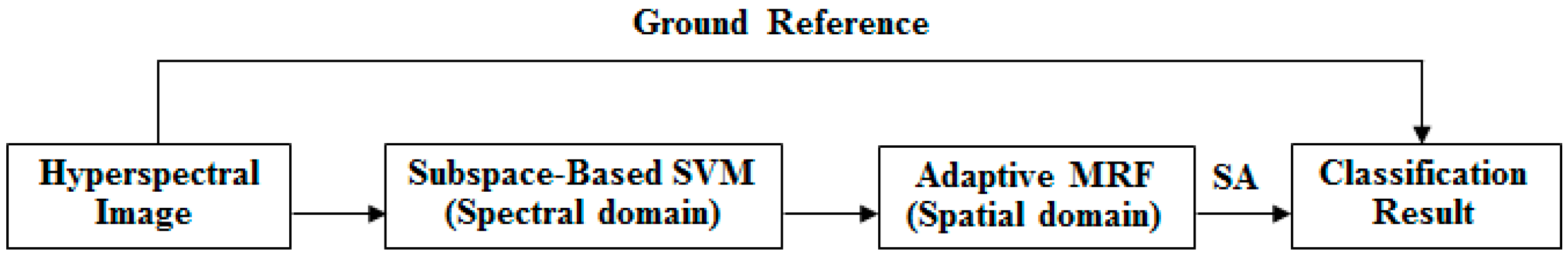
3. Proposed Method
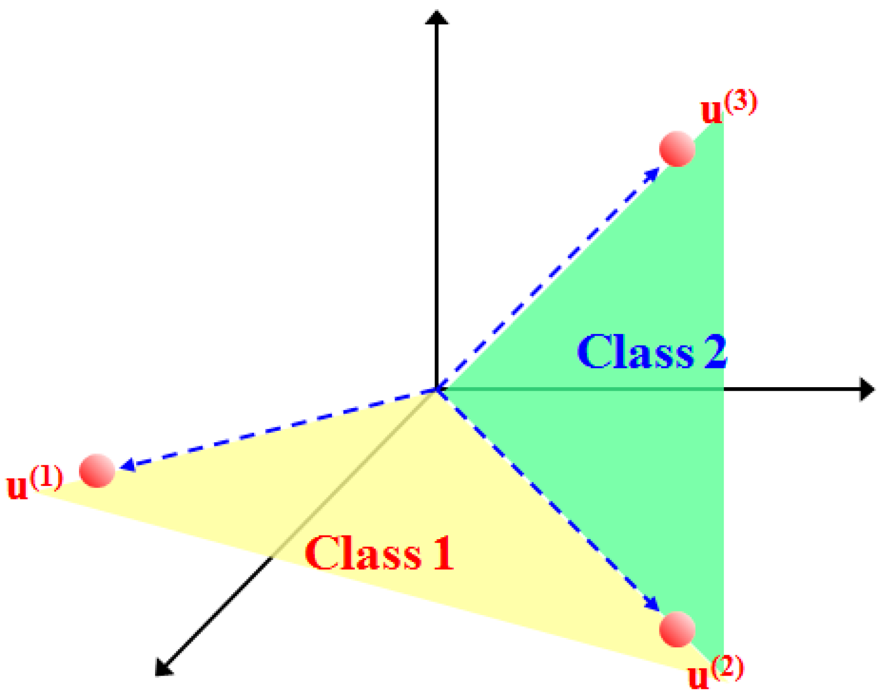
3.1. SVMsub
| Algorithm 1 SVMsub |
| Input: The available training data , their class labels , and the test sample set with class labels represented by . |
| for to do |
| ( computes the subspace according to Equations (7)–(9) ) |
| end |
| for to do |
| ( computes the projected samples according to Equations (10) and (11) ) |
| end |
| for to do |
| ( computes the SVM results according to Equation (12) ) |
| end |
| Output: The class labels . |
3.2. SVMsub-eMRF
| Algorithm 2 SVMsub-eMRF |
| Input: The available training data , their class labels , and the test sample set with class labels represented by . |
| Step 1: Compute the results of SVMsub according to Algorithm 1; |
| Step 2: Obtain the first principal component using the MNF transform; |
| Step 3: Detect the edges using the Canny or LoG detector and the results of Step 2; |
| Step 4: Define the thresholds and to determine the using the results of Step 3 according to Equations (16) and (17); |
| Step 5: Determine the final class labels according to Equation (18); |
| Output: The class labels . |
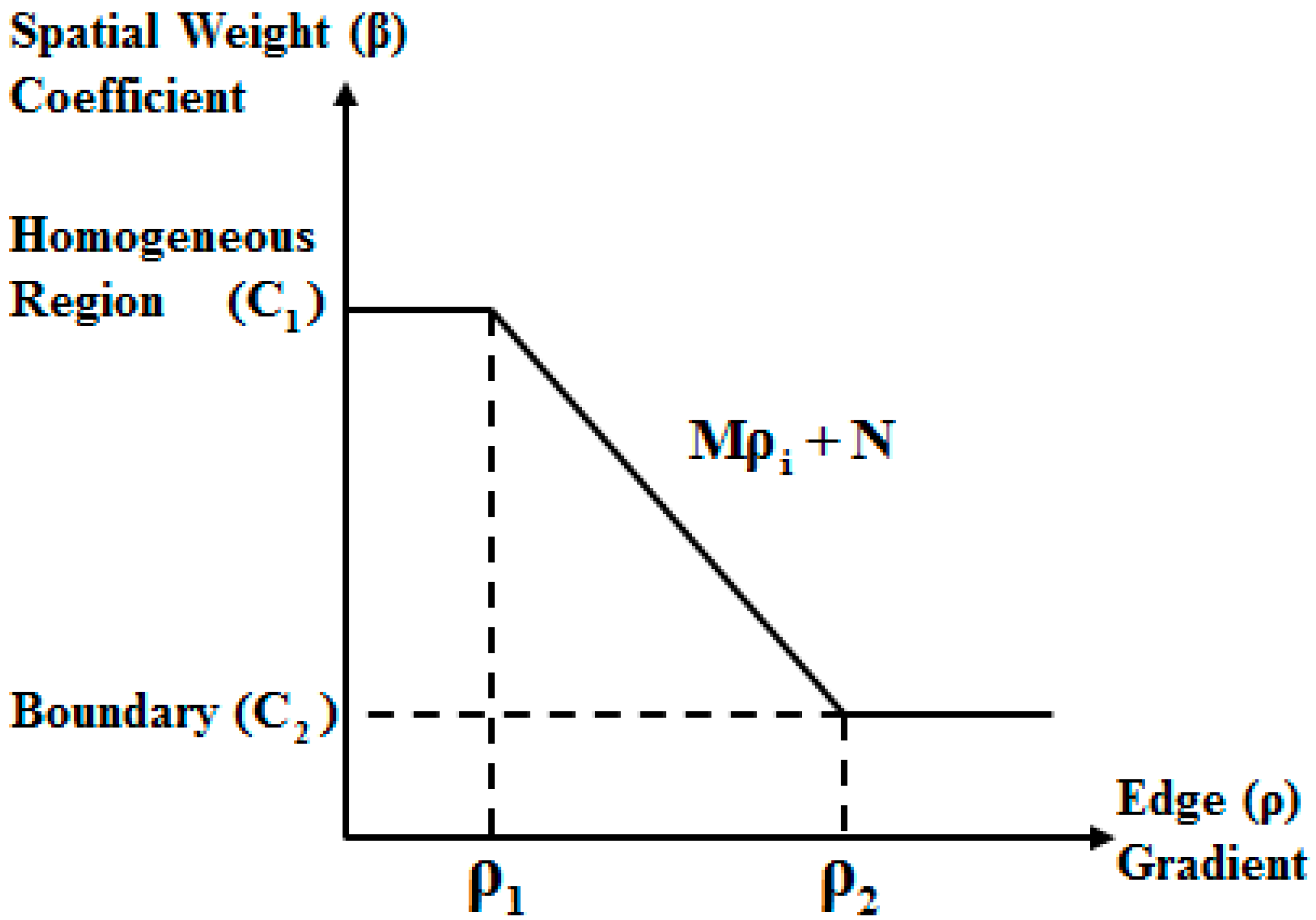
3.3. SVMsub-aMRF
| Algorithm 3 SVMsub-aMRF |
| Input: The available training data , their class labels , and the test sample set with class labels represented by . |
| Step 1: Compute the results of SVMsub according to Algorithm 1; |
| Step 2: Obtain the first principal component using the NAPC transform; |
| Step 3: Calculate the RHIs using the result of Step 1 and Step 2 according to Equation (19); |
| Step 4: Compute the using the results of Step 3 according to Equation (20); |
| Step 5: Determine the final class labels according to Equations (21) and (22); |
| Output: The class labels . |
4. Experiments
| Algorithm 4 SA Optimization |
| Input: The available training data , their class labels , and a lowest temperature . |
| Step 1: Obtain the initial energy function according to the results of SVMsub-eMRF or SVMsub-aMRF; |
| Step 2: Randomly vary the classes and calculate a new energy function ; |
| Step 3: Compute the difference between the results of Step 1 and Step 2: ; |
| Step 4: If , replace the class labels with the current ones. Otherwise, leave them unchanged; |
| Step 5: Return to Step 2 until the predefined lowest temperature has been reached; |
| Step 6: Determine the final class labels ; |
| Output: The class labels . |
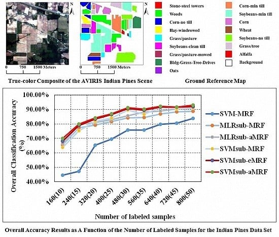
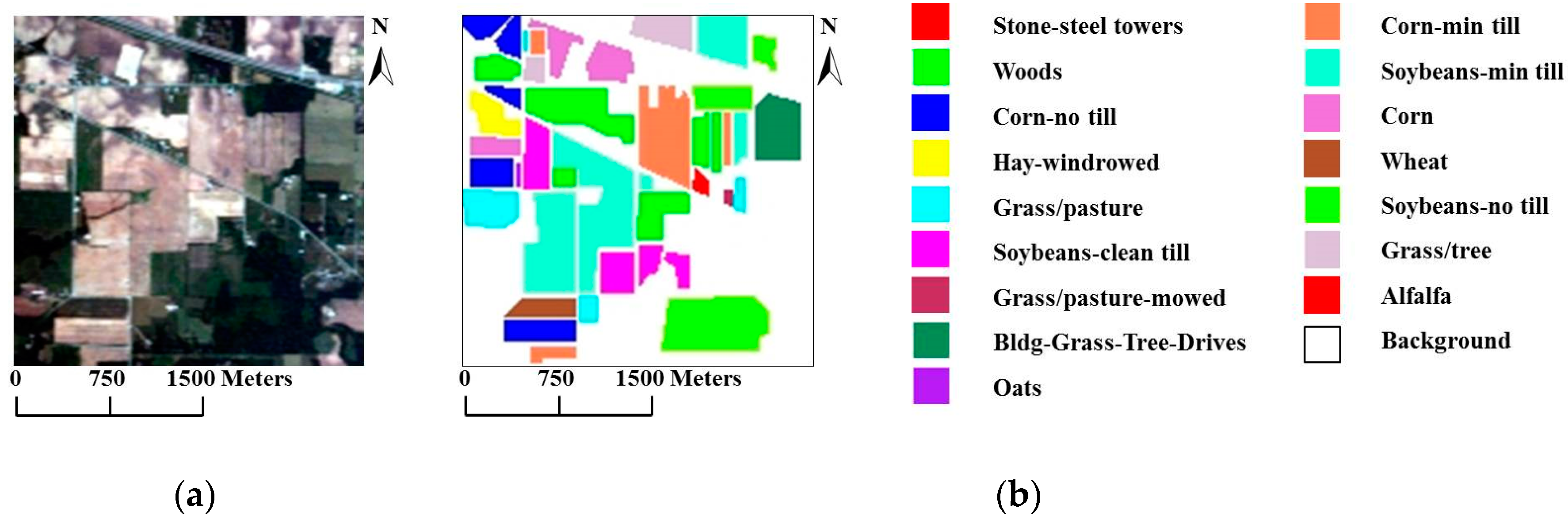
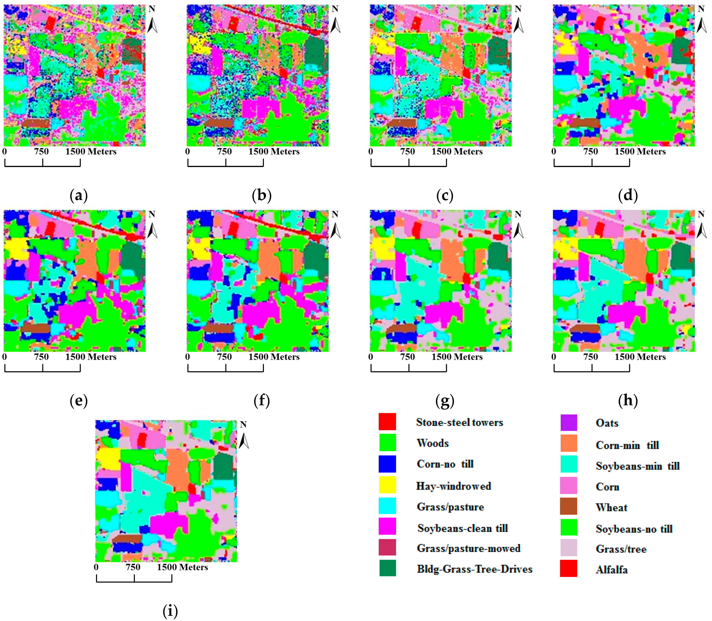
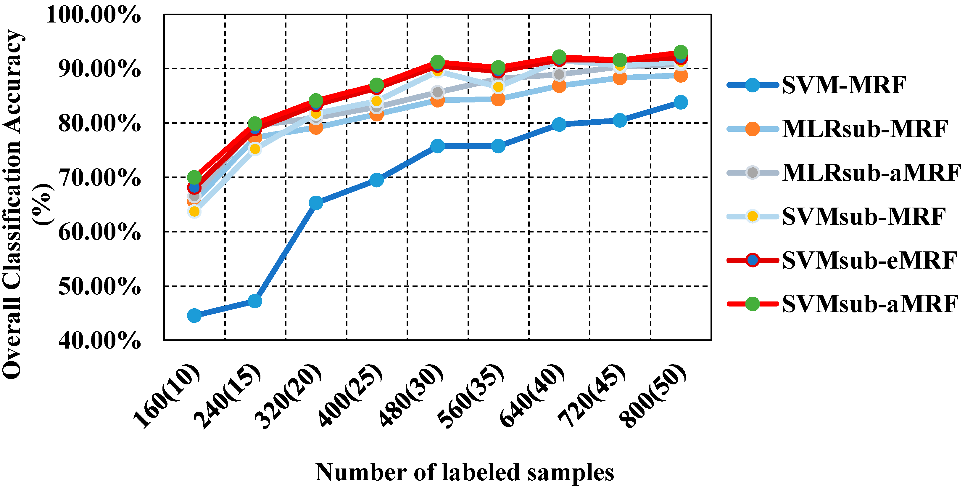
4.1. Experiments Using the AVIRIS Indian Pines Data Set
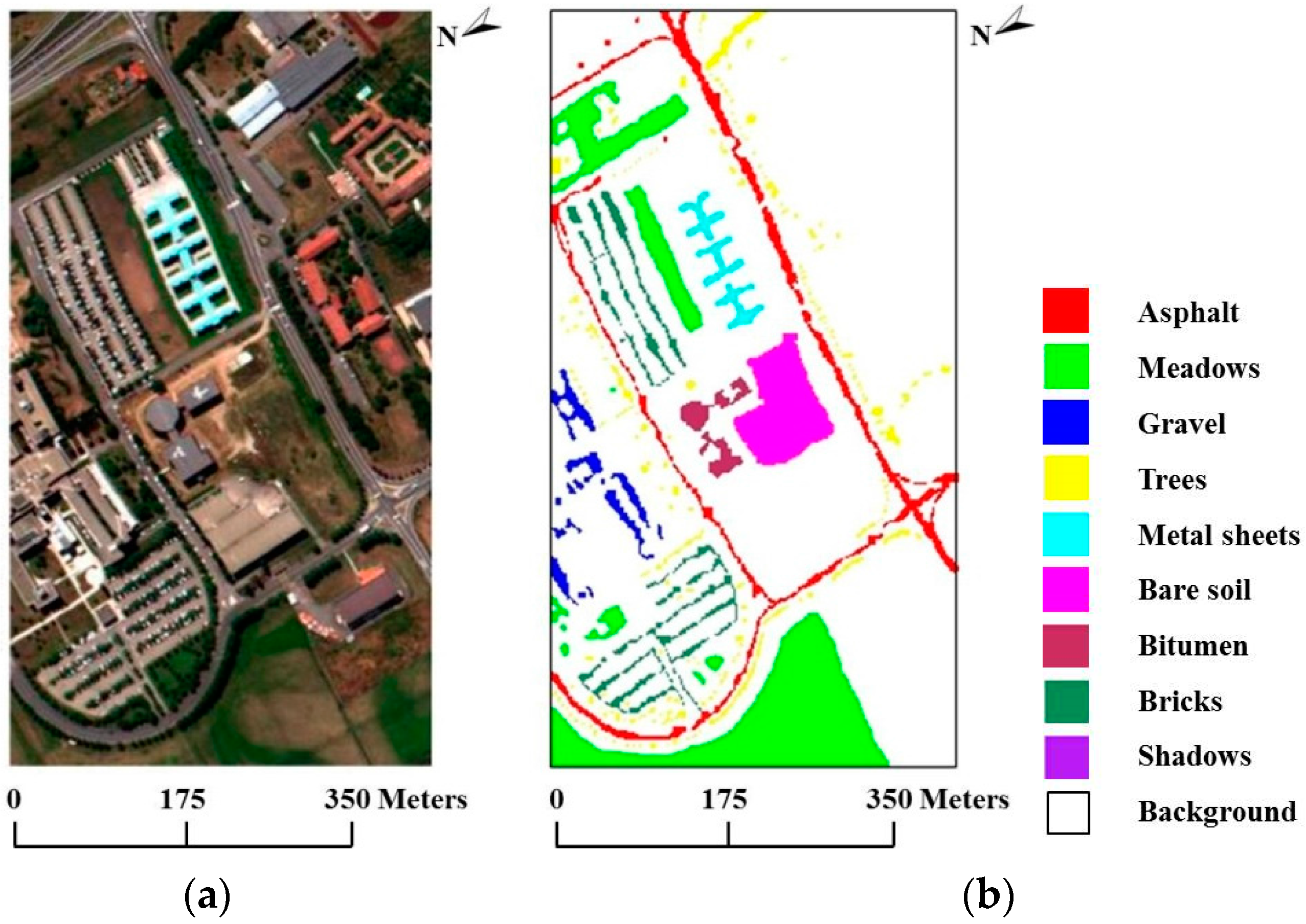
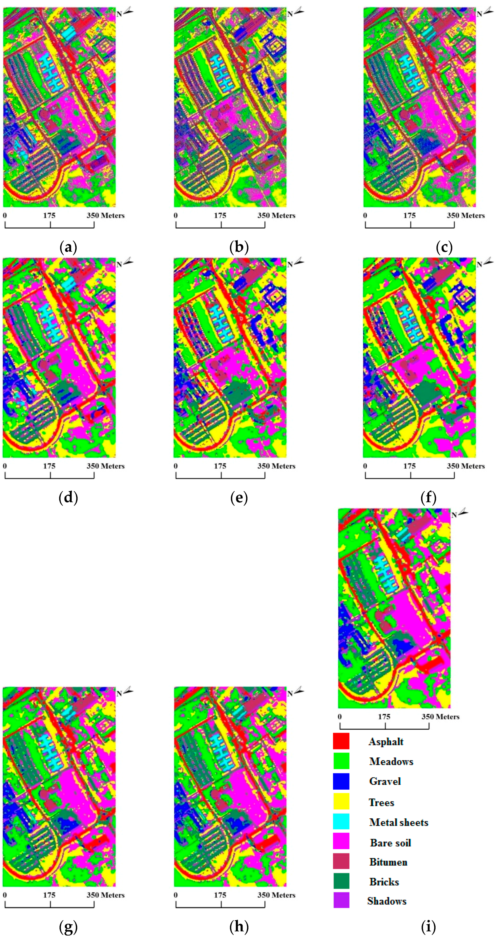
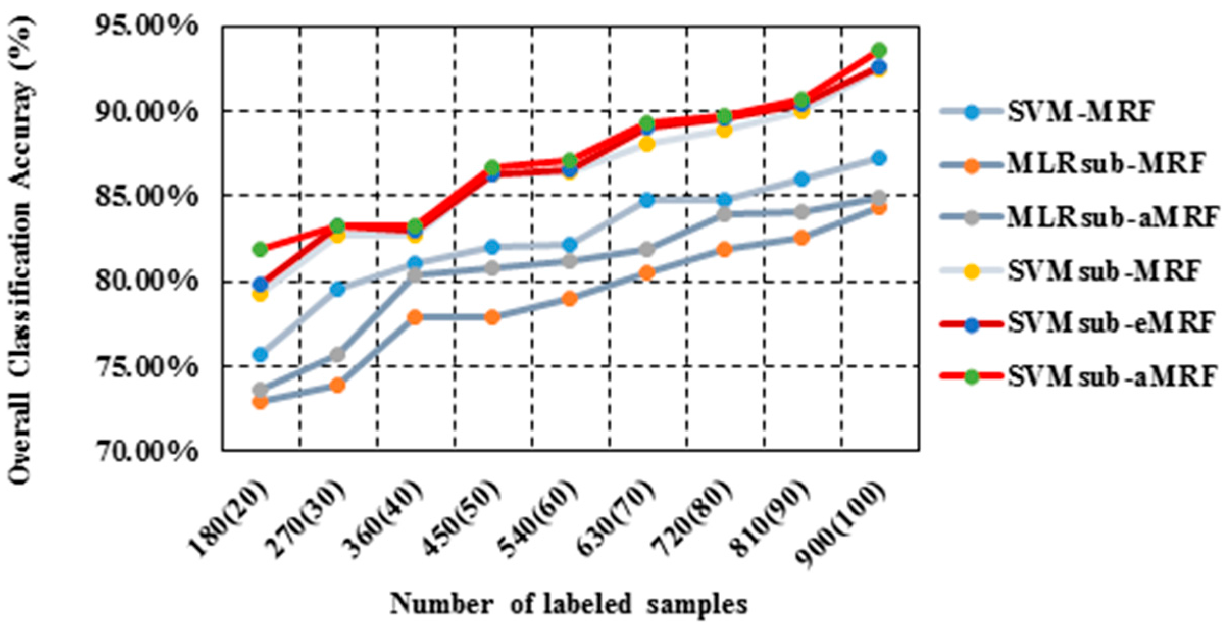
4.2. Experiments Using the ROSIS University of Pavia Data Set
5. Conclusions
Acknowledgments
Author Contributions
Conflicts of Interest
Abbreviations
| SVM | Support Vector Machine |
| MRF | Markov Random Field |
| SA | Simulated Annealing |
| MLR | Multinomial Logistic Regression |
| SVMsub | Subspace-based SVM |
| MLRsub | Subspace-based MLR |
| RHI | Relative Homogeneity Index |
| MAP | Maximum A Posteriori |
| eMRF | Edge-constrained MRF |
| aMRF | RHI-based Adaptive MRF |
| NAPC | Noise-Adjusted Principal Components |
| RBF | Radial Basis Function |
| MNF | Minimum Noise Fraction |
| LoG | Laplacian of Gaussian |
| OA | Overall Accuracy |
References
- Landgrebe, D.A. Signal Theory Methods in Multispectral Remote Sensing; Wiley: New York, NY, USA, 2003. [Google Scholar]
- Qian, Y.; Yao, F.; Jia, S. Band selection for hyperspectral imagery using affinity propagation. IET Comput. Vis. 2009, 3, 213–222. [Google Scholar] [CrossRef]
- Melgani, F.; Bruzzone, L. Classification of hyperspectral remote sensing images with support vector machines. IEEE Trans. Geosci. Remote Sens. 2004, 42, 1778–1790. [Google Scholar] [CrossRef]
- Schölkopf, B.; Smola, A.J. Learning with Kernels: Support Vector Machines, Regularization, Optimization, and Beyond; MIT Press: Cambridge, MA, USA, 2002. [Google Scholar]
- Harsanyi, J.C.; Chang, C. Hyperspectral image classification and dimensionality reduction: An orthogonal subspace projection approach. IEEE Trans. Geosci. Remote Sens. 1994, 32, 779–785. [Google Scholar] [CrossRef]
- Larsen, R.; Arngren, M.; Hansen, P.W.; Nielsen, A.A. Kernel based subspace projection of near infrared hyperspectral images of maize kernels. Image Anal. 2009, 5575, 560–569. [Google Scholar]
- Chen, W.; Huang, J.; Zou, J.; Fang, B. Wavelet-face based subspace LDA method to solve small sample size problem in face recognition. Int. J. Wavelets Multiresolut. Inf. Process. 2009, 7, 199–214. [Google Scholar] [CrossRef]
- Gao, L.; Li, J.; Khodadadzadeh, M.; Plaza, A.; Zhang, B.; He, Z.; Yan, H. Subspace-based support vector machines for hyperspectral image classification. IEEE Geosci. Remote Sens. Lett. 2015, 12, 349–353. [Google Scholar]
- Li, W.; Tramel, E.W.; Prasad, S.; Fowler, J.E. Nearest regularized subspace for hyperspectral classification. IEEE Trans. Geosci. Remote Sens. 2014, 52, 477–489. [Google Scholar] [CrossRef]
- Li, J.; Bioucas-Dias, J.M.; Plaza, A. Semisupervised hyperspectral image segmentation using multinomial logistic regression with active learning. IEEE Trans. Geosci. Remote Sens. 2010, 48, 4085–4098. [Google Scholar] [CrossRef]
- Fauvel, M.; Tarabalka, Y.; Benediktsson, J.A.; Chanussot, J.; Tilton, J.C. Advances in spectral-spatial classification of hyperspectral images. Proc. IEEE 2013, 101, 652–675. [Google Scholar] [CrossRef]
- Fauvel, M.; Benediktsson, J.A.; Chanussot, J.; Sveinsson, J.R. Spectral and spatial classification of hyperspectral data using SVMs and morphological profiles. IEEE Trans. Geosci. Remote Sens. 2008, 46, 3804–3814. [Google Scholar] [CrossRef]
- Jia, S.; Xie, Y.; Tang, G.; Zhu, J. Spatial-spectral-combined sparse representation-based classification for hyperspectral imagery. Soft Comput. 2014, 1–10. [Google Scholar] [CrossRef]
- Benediktsson, J.A.; Pesaresi, M.; Arnason, K. Classification and feature extraction for remote sensing images from urban areas based on morphological transformations. IEEE Trans. Geosci. Remote Sens. 2003, 41, 1940–1949. [Google Scholar] [CrossRef]
- Benediktsson, J.A.; Palmason, J.A.; Sveinsson, J.R. Classification of hyperspectral data from urban areas based on extended morphological profiles. IEEE Trans. Geosci. Remote Sens. 2005, 43, 480–491. [Google Scholar] [CrossRef]
- Li, J.; Bioucas-Dias, J.M.; Plaza, A. Spectral-spatial hyperspectral image segmentation using subspace multinomial logistic regression and Markov random fields. IEEE Trans. Geosci. Remote Sens. 2012, 50, 809–823. [Google Scholar] [CrossRef]
- Ni, L.; Gao, L.; Li, S.; Li, J.; Zhang, B. Edge-constrained Markov random field classification by integrating hyperspectral image with LiDAR data over urban areas. J. Appl. Remote Sens. 2014, 8. [Google Scholar] [CrossRef]
- Zhang, B.; Li, S.; Jia, X.; Gao, L.; Peng, M. Adaptive Markov random field approach for classification of hyperspectral imagery. IEEE Geosci. Remote Sens. Lett. 2011, 8, 973–977. [Google Scholar] [CrossRef]
- Kirkpatrick, S.; Gelatt, C.D.; Vecchi, M.P. Optimization by simulated annealing. Science 1983, 220, 671–680. [Google Scholar] [CrossRef] [PubMed]
- Camps-Valls, G.; Bruzzone, L. Kernel-based methods for hyperspectral image classification. IEEE Trans. Geosci. Remote Sens. 2005, 43, 1351–1362. [Google Scholar] [CrossRef]
- Xie, J.; Hone, K.; Xie, W.; Gao, X.; Shi, Y.; Liu, X. Extending twin support vector machine classifier for multi-category classification problems. Intell. Data Anal. 2013, 17, 649–664. [Google Scholar]
- Vapnik, V. Statistical Learning Theory; Wiley: New York, NY, USA, 1998. [Google Scholar]
- Richards, J.A.; Jia, X. Remote Sensing Digital Image Analysis: An Introduction; Springer-Verlag: Berlin, Germany, 2006. [Google Scholar]
- Plaza, A.; Benediktsson, J.A.; Boardman, J.W.; Brazile, J.; Bruzzone, L.; Camps-Valls, G.; Chanussot, J.; Fauvel, M.; Gamba, P.; Gualtieri, A. Recent advances in techniques for hyperspectral image processing. Remote Sens. Environ. 2009, 113, S110–S122. [Google Scholar] [CrossRef]
- Zhang, Y.; Brady, M.; Smith, S. Segmentation of brain MR images through a hidden Markov random field model and the expectation-maximization algorithm. IEEE Trans. Med. Imaging 2001, 20, 45–57. [Google Scholar] [CrossRef] [PubMed]
- Geman, S.; Geman, D. Stochastic relaxation, Gibbs distributions, and the Bayesian restoration of images. IEEE Trans. Pattern Anal. Mach. Intell. 1984, 6, 721–741. [Google Scholar] [CrossRef] [PubMed]
- Jia, X.; Richards, J.A. Managing the spectral-spatial mix in context classification using Markov random fields. IEEE Geosci. Remote Sens. Lett. 2008, 5, 311–314. [Google Scholar] [CrossRef]
- Chang, C.I. Hyperspectral Imaging: Techniques for Spectral Detection and Classification; Springer Science and Business Media: New York, NY, USA, 2003. [Google Scholar]
- Zhong, Y.; Lin, X.; Zhang, L. A support vector conditional random fields classifier with a Mahalanobis distance boundary constraint for high spatial resolution remote sensing imagery. IEEE J. Sel. Top. Appl. Earth Obs. Remote Sens. 2014, 7, 1314–1330. [Google Scholar] [CrossRef]
- Jiménez, L.O.; Rivera-Medina, J.L.; Rodríguez-Díaz, E.; Arzuaga-Cruz, E.; Ramírez-Vélez, M. Integration of spatial and spectral information by means of unsupervised extraction and classification for homogenous objects applied to multispectral and hyperspectral data. IEEE Trans. Geosci. Remote Sens. 2005, 43, 844–851. [Google Scholar] [CrossRef]
- Keshava, N.; Mustard, J.F. Spectral unmixing. IEEE Signal Process. Mag. 2002, 19, 44–57. [Google Scholar] [CrossRef]
- Bioucas-Dias, J.M.; Plaza, A.; Dobigeon, N.; Parente, M.; Du, Q.; Gader, P.; Chanussot, J. Hyperspectral unmixing overview: Geometrical, statistical, and sparse regression-based approaches. IEEE J. Sel. Top. Appl. Earth Obs. Remote Sens. 2012, 5, 354–379. [Google Scholar] [CrossRef]
- Scholkopf, B.; Sung, K.K.; Burges, C.J.C.; Girosi, F.; Niyogi, P.; Poggio, T.; Vapnik, V. Comparing support vector machines with Gaussian kernels to radial basis function classifiers. IEEE Trans. Signal Process. 1997, 45, 2758–2765. [Google Scholar] [CrossRef]
- Cristianini, N.; Shawe-Taylor, J. An Introduction to Support Vector Machines and Other Kernel-Based Learning Methods; Cambridge University Press: Cambridge, UK, 2000. [Google Scholar]
- Platt, J. Probabilistic outputs for support vector machines and comparisons to regularized likelihood methods. Adv. Large Margin Classif. 1999, 10, 61–74. [Google Scholar]
- Lin, H.; Lin, C.; Weng, R.C. A note on Platt’s probabilistic outputs for support vector machines. Mach. Learn. 2007, 68, 267–276. [Google Scholar] [CrossRef]
- Gillespie, A.R. Spectral mixture analysis of multispectral thermal infrared images. Remote Sens. Environ. 1992, 42, 137–145. [Google Scholar] [CrossRef]
- Green, A.A.; Berman, M.; Switzer, P.; Craig, M.D. A transformation for ordering multispectral data in terms of image quality with implications for noise removal. IEEE Trans. Geosci. Remote Sens. 1988, 26, 65–74. [Google Scholar] [CrossRef]
- Maini, R.; Aggarwal, H. Study and comparison of various image edge detection techniques. Int. J. Image Process. 2009, 3, 1–11. [Google Scholar]
- Tarabalka, Y.; Benediktsson, J.A.; Chanussot, J. Spectral-spatial classification of hyperspectral imagery based on partitional clustering techniques. IEEE Trans. Geosci. Remote Sens. 2009, 47, 2973–2987. [Google Scholar] [CrossRef]
- Farag, A.A.; Mohamed, R.M.; El-Baz, A. A unified framework for map estimation in remote sensing image segmentation. IEEE Trans. Geosci. Remote Sens. 2005, 43, 1617–1634. [Google Scholar] [CrossRef]
- Kirkpatrick, S. Optimization by simulated annealing: Quantitative studies. J. Stat. Phys. 1984, 34, 975–986. [Google Scholar] [CrossRef]


| Class | Samp-les | Spectral Space | Spectral-Spatial Space | |||||||
|---|---|---|---|---|---|---|---|---|---|---|
| SVM | MLRsub | SVMsub | SVM-MRF | MLRsub-MRF | MLRsub-aMRF | SVMsub-MRF | SVMsub-eMRF | SVMsub-aMRF | ||
| Alfalfa | 54 | 78.75% | 85.83% | 87.92% | 100.00% | 98.15% | 98.15% | 98.15% | 98.15% | 98.15% |
| Corn-no till | 1434 | 40.44% | 64.22% | 67.73% | 59.27% | 86.12% | 91.21% | 83.40% | 83.33% | 84.59% |
| Corn-min till | 834 | 43.21% | 60.99% | 67.71% | 59.95% | 70.74% | 84.53% | 77.58% | 83.21% | 80.22% |
| Corn | 234 | 66.39% | 77.60% | 86.14% | 99.57% | 99.57% | 97.86% | 100.00% | 98.72% | 100.00% |
| Grass/pasture | 497 | 75.22% | 84.07% | 87.47% | 89.54% | 93.36% | 91.55% | 92.56% | 94.77% | 95.98% |
| Grass/tree | 747 | 77.26% | 91.82% | 92.80% | 99.33% | 97.99% | 98.39% | 97.59% | 97.59% | 97.99% |
| Grass/pasture-mowed | 26 | 84.62% | 86.15% | 87.69% | 92.31% | 100.00% | 92.31% | 84.62% | 92.31% | 96.15% |
| Hay-windrowed | 489 | 81.15% | 95.46% | 96.52% | 79.75% | 99.39% | 99.18% | 99.18% | 98.77% | 98.57% |
| Oats | 20 | 71.00% | 94.00% | 82.00% | 100.00% | 100.00% | 100.00% | 100.00% | 90.00% | 100.00% |
| Soybeans-no till | 968 | 51.93% | 61.46% | 66.88% | 76.65% | 95.66% | 91.53% | 93.08% | 95.66% | 96.69% |
| Soybeans-min till | 2468 | 52.78% | 44.33% | 72.16% | 64.02% | 65.36% | 65.36% | 84.08% | 85.53% | 87.60% |
| Soybeans-clean till | 614 | 50.38% | 67.84% | 82.35% | 72.64% | 88.60% | 93.97% | 95.44% | 95.28% | 99.19% |
| Wheat | 212 | 93.25% | 99.56% | 99.23% | 99.53% | 100.00% | 99.06% | 99.53% | 99.53% | 100.00% |
| Woods | 1294 | 75.89% | 95.59% | 90.27% | 94.67% | 99.15% | 99.38% | 94.28% | 94.74% | 96.60% |
| Bldg-Grass-Tree-Drives | 380 | 50.65% | 36.46% | 68.87% | 77.63% | 56.84% | 52.37% | 90.79% | 88.68% | 80.79% |
| Stone-steel towers | 95 | 96.30% | 90.73% | 91.51% | 96.84% | 100.00% | 100.00% | 97.89% | 98.95% | 97.89% |
| Overall accuracy statistic | 58.47% | 67.62% | 77.78% | 75.72% | 84.20% | 85.66% | 89.49% | 90.57% | 91.22% | |
| 0.53 | 0.64 | 0.75 | 0.73 | 0.82 | 0.84 | 0.88 | 0.89 | 0.90 | ||
| Class | Samp-les | Spectral Space | Spectral-Spatial Space | |||||||
|---|---|---|---|---|---|---|---|---|---|---|
| SVM | MLRsub | SVMsub | SVM-MRF | MLRsub-MRF | MLRsub-aMRF | SVMsub-MRF | SVMsub-eMRF | SVMsub-aMRF | ||
| Alfalfa | 54 | 91.59% | 78.99% | 89.89% | 98.15% | 98.15% | 98.15% | 94.44% | 96.30% | 96.30% |
| Corn-no till | 1434 | 55.82% | 56.85% | 66.84% | 60.11% | 68.34% | 67.99% | 72.87% | 72.52% | 75.45% |
| Corn-min till | 834 | 58.60% | 61.22% | 72.21% | 76.98% | 80.22% | 83.69% | 85.73% | 90.41% | 91.13% |
| Corn | 234 | 76.98% | 70.74% | 86.53% | 97.44% | 94.87% | 97.01% | 99.57% | 97.44% | 98.72% |
| Grass/pasture | 497 | 86.64% | 84.75% | 89.86% | 93.76% | 95.17% | 97.18% | 90.34% | 93.36% | 95.77% |
| Grass/tree | 747 | 85.92% | 90.43% | 94.85% | 93.71% | 98.13% | 99.33% | 98.80% | 99.06% | 99.20% |
| Grass/pasture-mowed | 26 | 92.31% | 90.77% | 90.77% | 100.00% | 100.00% | 100.00% | 96.15% | 100.00% | 100.00% |
| Hay-windrowed | 489 | 92.28% | 95.48% | 96.14% | 98.77% | 99.18% | 99.18% | 99.18% | 98.16% | 98.57% |
| Oats | 20 | 88.00% | 88.00% | 86.00% | 100.00% | 100.00% | 100.00% | 50.00% | 100.00% | 90.00% |
| Soybeans-no till | 968 | 69.47% | 59.26% | 72.70% | 77.38% | 79.75% | 87.29% | 90.08% | 91.43% | 88.02% |
| Soybeans-min till | 2468 | 65.35% | 44.70% | 67.50% | 85.78% | 62.60% | 64.14% | 77.19% | 77.39% | 78.73% |
| Soybeans-clean till | 614 | 62.85% | 66.76% | 82.20% | 83.22% | 74.92% | 69.06% | 96.25% | 94.46% | 98.21% |
| Wheat | 212 | 95.91% | 99.45% | 99.45% | 100.00% | 99.53% | 99.53% | 100.00% | 99.53% | 99.53% |
| Woods | 1294 | 85.98% | 85.28% | 91.38% | 89.10% | 97.76% | 96.06% | 98.22% | 97.53% | 97.84% |
| Bldg-Grass-Tree-Drives | 380 | 60.62% | 45.39% | 61.71% | 83.95% | 61.05% | 71.84% | 67.11% | 76.05% | 76.32% |
| Stone-steel towers | 95 | 96.28% | 91.32% | 91.01% | 100.00% | 100.00% | 100.00% | 97.89% | 98.95% | 98.95% |
| Overall accuracy statistic | 71.01% | 65.19% | 77.56% | 83.31% | 79.51% | 80.87% | 86.34% | 87.16% | 88.04% | |
| 0.67 | 0.61 | 0.75 | 0.81 | 0.77 | 0.78 | 0.85 | 0.86 | 0.86 | ||
| Samples (per Class) | Classification Method | ||||||
|---|---|---|---|---|---|---|---|
| SVM-MRF | MLRsub-MRF | MLRsub-aMRF | SVMsub-MRF | SVMsub-eMRF | SVMsub-aMRF | ||
| 160 (10) | OA (Time) | 44.56% (2.83) | 65.58% (2.70) | 66.52% (2.71) | 63.70% (0.89) | 68.10% (0.99) | 69.98% (0.89) |
| statistic | 0.3847 | 0.6188 | 0.6296 | 0.6000 | 0.6457 | 0.6667 | |
| 240 (15) | OA (Time) | 47.19% (3.60) | 77.32% (3.23) | 79.49% (3.23) | 75.21% (0.93) | 78.92% (1.03) | 79.90% (0.94) |
| statistic | 0.4208 | 0.7430 | 0.7670 | 0.7217 | 0.7635 | 0.7736 | |
| 320 (20) | OA (Time) | 65.28% (4.56) | 79.15% (3.43) | 80.95% (3.43) | 81.74% (0.95) | 83.35% (1.05) | 84.14% (0.96) |
| statistic | 0.6098 | 0.7628 | 0.7802 | 0.7921 | 0.8104 | 0.8193 | |
| 400 (25) | OA (Time) | 69.47% (5.68) | 81.64% (3.46) | 82.94% (3.47) | 84.03% (0.97) | 86.49% (1.07) | 87.02% (0.97) |
| statistic | 0.6551 | 0.7908 | 0.8068 | 0.8186 | 0.8441 | 0.8517 | |
| 480 (30) | OA (Time) | 75.72% (6.94) | 84.20% (3.66) | 85.66% (3.68) | 89.49% (0.99) | 90.57% (1.09) | 91.22% (1.00) |
| statistic | 0.7274 | 0.8219 | 0.8387 | 0.8809 | 0.8931 | 0.9003 | |
| 560 (35) | OA (Time) | 75.75% (8.23) | 84.42% (3.98) | 88.18% (3.99) | 86.63% (1.01) | 89.54% (1.12) | 90.23% (1.02) |
| statistic | 0.7281 | 0.8237 | 0.8658 | 0.8525 | 0.8815 | 0.8909 | |
| 640 (40) | OA (Time) | 79.73% (9.73) | 86.86% (4.06) | 88.90% (4.07) | 91.55% (1.05) | 91.63% (1.16) | 92.20% (1.05) |
| statistic | 0.7701 | 0.8488 | 0.8724 | 0.9037 | 0.9046 | 0.9110 | |
| 720 (45) | OA (Time) | 80.47% (11.69) | 88.35% (4.38) | 90.34% (4.39) | 90.54% (1.07) | 91.57% (1.18) | 91.61% (1.08) |
| statistic | 0.7787 | 0.8670 | 0.8898 | 0.8922 | 0.9040 | 0.9046 | |
| 800 (50) | OA (Time) | 83.79% (14.40) | 88.74% (4.64) | 90.83% (4.65) | 91.28% (1.12) | 91.94% (1.22) | 93.03% (1.13) |
| statistic | 0.8164 | 0.8708 | 0.8957 | 0.9011 | 0.9088 | 0.9195 | |
| Class | Samples | Spectral Space | Spectral-Spatial Space | ||||||||
|---|---|---|---|---|---|---|---|---|---|---|---|
| Train | Test | SVM | MLR-sub | SVM-sub | SVM-MRF | MLRsub-MRF | MLRsub-aMRF | SVMsub-MRF | SVMsub-eMRF | SVMsub-aMRF | |
| Alfalfa | 540 | 6631 | 63.64% | 43.01% | 63.52% | 76.05% | 66.75% | 73.15% | 70.96% | 73.16% | 83.60% |
| Bare soil | 548 | 18,649 | 57.86% | 71.11% | 61.82% | 60.19% | 69.25% | 69.90% | 68.61% | 69.13% | 69.08% |
| Bitumen | 392 | 2099 | 82.28% | 62.12% | 85.99% | 88.49% | 44.27% | 37.70% | 95.20% | 91.84% | 97.15% |
| Bricks | 524 | 3064 | 97.00% | 91.25% | 96.38% | 97.35% | 97.06% | 96.77% | 96.27% | 95.05% | 93.60% |
| Gravel | 265 | 1345 | 99.41% | 98.66% | 98.96% | 99.85% | 99.13% | 99.78% | 99.64% | 98.77% | 99.71% |
| Meadows | 532 | 5029 | 72.72% | 62.95% | 77.49% | 82.92% | 77.06% | 68.95% | 86.93% | 87.79% | 90.73% |
| Metal sheets | 375 | 1330 | 91.05% | 84.51% | 80.00% | 97.20% | 91.67% | 97.27% | 91.52% | 91.96% | 96.31% |
| Shadows | 514 | 3682 | 80.28% | 49.29% | 76.10% | 91.49% | 68.51% | 74.45% | 93.37% | 96.31% | 94.46% |
| Trees | 231 | 947 | 99.89% | 100.00% | 99.58% | 99.81% | 100.00% | 100.00% | 99.71% | 99.42% | 94.46% |
| Overall accuracy statistic | 69.70% | 66.84% | 71.38% | 75.71% | 72.97% | 73.67% | 79.20% | 79.84% | 81.94% | ||
| 0.63 | 0.58 | 0.65 | 0.70 | 0.66 | 0.67 | 0.74 | 0.75 | 0.78 | |||
| Samples (per Class) | Classification Method | ||||||
|---|---|---|---|---|---|---|---|
| SVM-MRF | MLRsub-MRF | MLRsub-aMRF | SVMsub-MRF | SVMsub-eMRF | SVMsub-aMRF | ||
| 180 (20) | OA (Time) | 75.71% (9.05) | 72.97% (5.97) | 73.67% (5.99) | 79.20% (3.12) | 79.84% (4.17) | 81.94% (3.14) |
| statistic | 0.7021 | 0.6632 | 0.6693 | 0.7415 | 0.7491 | 0.7751 | |
| 270 (30) | OA (Time) | 79.59% (11.34) | 73.96% (6.13) | 75.66% (6.16) | 82.67% (3.20) | 83.20% (4.25) | 83.30% (3.23) |
| statistic | 0.7496 | 0.6728 | 0.6938 | 0.7806 | 0.7875 | 0.7885 | |
| 360 (40) | OA (Time) | 80.99% (12.36) | 77.82% (6.27) | 80.37% (6.30) | 82.68% (3.27) | 82.98% (4.34) | 83.23% (3.30) |
| statistic | 0.7669 | 0.7143 | 0.7477 | 0.7844 | 0.7863 | 0.7909 | |
| 450 (50) | OA (Time) | 81.95% (13.05) | 77.88% (6.39) | 80.75% (6.41) | 86.23% (3.33) | 86.24% (4.46) | 86.68% (3.41) |
| statistic | 0.7772 | 0.7208 | 0.7513 | 0.8261 | 0.8263 | 0.8318 | |
| 540 (60) | OA (Time) | 82.14% (14.05) | 78.98% (6.55) | 81.12% (6.60) | 86.37% (3.41) | 86.57% (4.55) | 87.15% (3.50) |
| statistic | 0.7795 | 0.7349 | 0.7611 | 0.8280 | 0.8305 | 0.8375 | |
| 630 (70) | OA (Time) | 84.77% (15.30) | 80.44% (6.60) | 81.91% (6.64) | 88.04% (3.50) | 88.98% (4.68) | 89.35% (3.62) |
| statistic | 0.8105 | 0.746 | 0.7644 | 0.8471 | 0.8588 | 0.8636 | |
| 720 (80) | OA (Time) | 84.83% (16.35) | 81.83% (6.73) | 83.90% (6.75) | 88.93% (3.61) | 89.54% (4.79) | 89.66% (3.71) |
| statistic | 0.8107 | 0.7661 | 0.7926 | 0.8594 | 0.8668 | 0.8682 | |
| 810 (90) | OA (Time) | 85.94% (17.29) | 82.58% (6.95) | 84.12% (6.99) | 90.03% (3.75) | 90.35% (4.87) | 90.69% (3.83) |
| statistic | 0.8240 | 0.7774 | 0.7960 | 0.8723 | 0.8764 | 0.8806 | |
| 900 (100) | OA (Time) | 87.28% (18.76) | 84.32% (7.01) | 84.93% (7.03) | 92.51% (3.87) | 92.61% (4.99) | 93.50% (3.95) |
| statistic | 0.8400 | 0.7977 | 0.8051 | 0.9036 | 0.9048 | 0.9162 | |
© 2016 by the authors; licensee MDPI, Basel, Switzerland. This article is an open access article distributed under the terms and conditions of the Creative Commons Attribution (CC-BY) license (http://creativecommons.org/licenses/by/4.0/).
Share and Cite
Yu, H.; Gao, L.; Li, J.; Li, S.S.; Zhang, B.; Benediktsson, J.A. Spectral-Spatial Hyperspectral Image Classification Using Subspace-Based Support Vector Machines and Adaptive Markov Random Fields. Remote Sens. 2016, 8, 355. https://doi.org/10.3390/rs8040355
Yu H, Gao L, Li J, Li SS, Zhang B, Benediktsson JA. Spectral-Spatial Hyperspectral Image Classification Using Subspace-Based Support Vector Machines and Adaptive Markov Random Fields. Remote Sensing. 2016; 8(4):355. https://doi.org/10.3390/rs8040355
Chicago/Turabian StyleYu, Haoyang, Lianru Gao, Jun Li, Shan Shan Li, Bing Zhang, and Jón Atli Benediktsson. 2016. "Spectral-Spatial Hyperspectral Image Classification Using Subspace-Based Support Vector Machines and Adaptive Markov Random Fields" Remote Sensing 8, no. 4: 355. https://doi.org/10.3390/rs8040355