Scale-Aware Pansharpening Algorithm for Agricultural Fragmented Landscapes

Abstract

Remote sensing (RS) has played an important role in extensive agricultural monitoring and management for several decades. However, the current spatial resolution of satellite imagery does not have enough definition to generalize its use in highly-fragmented agricultural landscapes, which represents a significant percentage of the world’s total cultivated surface. To characterize and analyze this type of landscape, multispectral (MS) images with high and very high spatial resolutions are required. Multi-source image fusion algorithms are normally used to improve the spatial resolution of images with a medium spatial resolution. In particular, pansharpening (PS) methods allow one to produce high-resolution MS images through a coherent integration of spatial details from a panchromatic (PAN) image with spectral information from an MS. The spectral and spatial quality of source images must be preserved to be useful in RS tasks. Different PS strategies provide different trade-offs between the spectral and the spatial quality of the fused images. Considering that agricultural landscape images contain many levels of significant structures and edges, the PS algorithms based on filtering processes must be scale-aware and able to remove different levels of detail in any input images. In this work, a new PS methodology based on a rolling guidance filter (RGF) is proposed. The main contribution of this new methodology is to produce artifact-free pansharpened images, improving the MS edges with a scale-aware approach. Three images have been used, and more than 150 experiments were carried out. An objective comparison with widely-used methodologies shows the capability of the proposed method as a powerful tool to obtain pansharpened images preserving the spatial and spectral information.

1. Introduction

Remote sensing (RS) is a widely-used tool to support decision making in agricultural censuses, land use assessments and crop monitoring. Most RS methods for crop mapping rely on low spatial resolution images, achieving good results when addressing large and homogeneous areas, but they are limited for crop identification and characterization at the farm level [1,2].

According to Lowder et al. [3], about 75% of the world’s 570 million farms are family concerns of less than 2 ha. This implies a highly fragmented agricultural landscape with a high spatial heterogeneity produced by the diversity in sizes, shapes and crops of the different agricultural plots. Under this scenario, agricultural studies using remote sensing techniques are conditioned upon the spatial resolution of the images; thus higher resolutions allow a more accurate analyses of the agricultural fields in most cases [4].

To address this requirement, continuous improvements in Earth observation technologies from space have resulted in a wide range of commercial satellites that offer a new generation of images that can simultaneously acquire both panchromatic (PAN) and multispectral (MS) imagery. The most popular optical satellites and their spatial resolutions are detailed in

Table 1. Commercial optical satellites that offer images with high and very high spatial resolutions.

Satellite	Spatial Resolution (m)
	Panchromatic (PAN)	Multispectral (MS)
Spot–6/7	1.50	6.00
QuickBird–2	0.65	2.60
Pleiades–1/2	0.50	2.00
WorldView–1/2	0.46	1.84
GeoEye–1	0.46	1.84
GeoEye–2	0.34	1.36
WorldView–3	0.31	1.24

.

Considering that in RS, PAN and MS images are acquired simultaneously over the same area, for each satellite, the information recorded is complementary for each satellite. To make the most of this complementarity, data fusion techniques provide the formal framework necessary to exploit the synergy that may exist between the different information sources or sensors, reducing redundant data and, at the same time, highlighting the most important information. Specifically, the objective of pansharpening (PS) is to fuse a low-resolution MS image with a high-resolution PAN image, to create a high-resolution MS image, subject to preserve both the spatial and spectral quality of the source images to be useful in RS tasks (e.g., feature extraction, segmentation, classification).

Even when an increase in the spatial resolution simplifies problems such as mixing pixels, other problems emerge due to the greater spatial variability for each spectral class present in the image; furthermore, the limited number of spectral bands of high and very high spatial resolution images produces a low separability between land covers [5]. This put a higher demand on the quality of pansharpened images and, therefore, on the PS technique itself [6].

Many PS algorithms are available today [7,8,9,10,11,12]; most of them follow two approaches [8,9]: component substitution (CS) and multi-resolution analysis (MRA). The former includes widely-used PS algorithms, such as: intensity-hue-saturation (IHS) [13], principal component analysis (PCA) [14], Grand-Schmidt (GS) [15] and Brovey transform (BT) [16]. Most of these techniques provide superior visual high-resolution multispectral images, but ignore the need for a high-quality synthesis of spectral information [9]. The MRA is based on the multi-resolution decomposition of the PAN image, with the aim of extracting its spatial details, which are injected into the MS image. Most of these approaches use the discrete wavelet transform (DWT), both in its pyramidal and redundant versions [5]. Even though these methods increase the spatial resolution of the MS images to the spatial resolution levels of PAN images, maintaining their spectral characteristics, they tend to accentuate the problem of injecting false details into the fused images even more [17]. Another strategy of the MRA approach is the use of the modulation transfer function (MTF) [18]. The novelty of the method relies on the fact that filters matching the MTFs of the different channels of the imaging instruments are used to extract the spectral (low pass) and spatial (high pass) information from the merged image. However, Massip et al. [19] concluded that the differences in sampling rates, pixel size, integration time and spectral sensitivity, between the MS and PAN sensors yield a difference in MTF. This difference must be taken into account when synthesizing MS images at the PAN high-spatial resolution. For a recent and more in-deep revision of some popular and state-of-the-art fusion methods at different levels, especially at the pixel level, see [20].

To reduce the problem of false details (artifacts), a PS algorithm, called WATFRAC, using fractal dimension maps as gain weighting, reified through the wavelet à trous transforms (WAT) method, was proposed by Lillo-Saavedra et al. [5]. The results showed that the images pansharpened using WATFRAC, as well as their classifications were of greater quality than images merged through the standard WAT method. However, the high computational cost of calculating the fractal dimension maps is a significant limitation when applying this methodology over large images.

Kaplan and Erer [21] recently proposed to decompose the PAN image using an edge-preserving method, which will decrease the amount of redundant high-frequency injection. The missing high-frequency information of the MS image is obtained by the decomposition of the PAN image using a bilateral filter [22]. The bilateral filter is a non-linear technique whose objective is to preserve the high-contrast edges and remove low-contrast or gradual changes. Kaplan and Erer [21] compared the results obtained by their algorithm, based on bilateral filtering, with the PS algorithm based on WAT. The results and conclusions showed that the PS method based on the multi-scale bilateral filter had better performance. In Hu and Li [23], a multi-sensor image fusion based on the multi-scale directional bilateral filter was proposed. The methodology combines the characteristic of the preserving edge of the bilateral filter with the ability to capture directional information from the non-subsampled directional filter bank, which is used to merge multi-sensor images. Using visible and infrared images, together with medical images, the authors demonstrated the superiority of their method compared with conventional methods (DWT, stationary wavelet transform and dual-tree complex wavelet transform) in terms of visual inspection and objective measures. Although bilateral filters consider some essential aspects in solving many image processing problems [22] (e.g., invariant feature construction, object classification, segmentation), their main drawback is not taking the scale into account (it is not a scale-aware process). This becomes important when the goal is to analyze landscapes, such as agricultural areas, as the objects in the image contain structures of various scales. Small structures, usually referred to as details, represent content classified as texture, small objects and noise, while large-scale information generally encompasses boundaries, slow spatial color transition and flat regions.

Considering the advantages of a guided filter (GF) demonstrated in He et al. [24], a new PS algorithm based on GF has recently been proposed in Liu and Liang [25]. The main contribution of this work is that it can use the PAN and MS images as input and guidance images, respectively, and the missing spatial information of the MS image can be obtained through the differences between the PAN and filtered images. Like bilateral filters, this algorithm is not considered an effective scale-aware filter, preventing the removal of different levels of detail in the input image.

The rolling guidance filter (RGF) [26] is a new framework of the scale-aware filter that can remove different levels of detail in natural images with the complete control of detail smoothing. The method is simple to implement, easy to understand, fully extensible to accommodate various data operations and quick to produce results, which is why it is a good alternative to be used for PS.

The agricultural landscape contains many levels of significant structures and edges [4], as well as high spatial heterogeneity within the agricultural plot; on the other hand, the plot boundaries are also relatively stable, while the cropping pattern is spatially highly variable [27]. This situation justifies the suitability of RGF to be used as a tool for developing a PS algorithm that considers the effective scale-aware issue, allowing different levels of detail in source images to be removed effectively and at a low computational cost.

In this work, a new PS methodology using an MRA approach and based on RGF is proposed. The main contribution of this new methodology is to produce artifact-free high spatial resolution pansharpened images, improving the MS edges by becoming aware of the scale (scale-aware) in images with a predominantly agricultural landscape. The performance of this method was compared with the WATFRAC, BT, GS, IHS and MTF-GLP (MTF using generalized Laplacian pyramid) [28] algorithms and evaluated using a set of spectral, spatial and overall quality indices [7,8]. The set of quality indices was summarized and compared using the Borda count (BC) method [29,30].

2. Background

The proposed PS methodology is based on RGF using an MRA approach. In this sense, a brief PS based on the MRA approach and RGF background is addressed in this section.

2.1. Pansharpening Based on the Multi-Resolution Approach

For the PS based on the MRA approach, most algorithms use the generalized Laplacian pyramid, the discrete wavelet transform and the contourlet transform, among others [31]. The basic idea is to extract the spatial detail information from the PAN image, not present in the low-resolution MS image, to inject it into the latter. The spatial detail of the PAN is obtained by the difference between the PAN and its low-pass version [8,25]. A general PS model based on the MRA is formalized in Equation (1):

$$P{S}_k={\widetilde{MS}}_k+g_k\times (PAN-PA{N}^{\prime })$$

(1)

where k indicates the k-th band, $\widetilde{MS}$ corresponds to the MS image interpolated on the PAN scale, $PA{N}^{\prime }$ to the low-pass version of PAN achieved by an iterative decomposition scheme and $g_k$ the injection gain for the k-th band.

The injection gain is a modulation of the spatial details through an element-by-element multiplication from the PAN to be integrated with the MS image to obtain the pansharpened image. There is a plethora of injection gain definitions [5,8,11,32,33].

In general, it is possible to define a PAN-sized matrix with all elements equal to one, injecting the total spatial detail. Other choices are the details being weighted by the ratio between the up-sampled MS ($\widetilde{MS}$) image and that of the low-pass filtered PAN, in order to reproduce the local intensity contrast of the PAN image in the pansharpened image. However, in this case, there is a unique low-pass filtered PAN for all bands [8]. Another approximation to define the $g_k$ (where k indicates the k-th band) was proposed by Otazu et al. [34] and developed for the wavelet-based method, called the additive wavelet luminance proportional (AWLP), formalized in Equation (2).

$$g_k=\frac{\widetilde{M{S}_k}}{\frac{1}{\#Bands}{\sum }_{i=1}^{\#Bands}\widetilde{M{S}_i}}$$

(2)

where $\#Bands$ denotes the number of bands in the MS image. In the work by Lillo-Saavedra et al. [5], a $g_k$, based on a fractal dimension map approach, was proposed. The aim of this proposal was to reduce the artifacts present in the pansharpened images. However, the high computational cost to calculate the fractal dimension maps is a drawback when used in large images. In order to reduce this computational cost, it is possible to use an approximation based on the entropy map (S) of the average of $M{S}_k$ and $PA{N}_K$, fulfilling the same purpose [35] (Equation (3)).

$$g_k=\frac{S\left(M{S}_k\right)+S\left(PA{N}_k\right)}{2}$$

(3)

where each element of the $g_k$ matrix contains the indexed entropy value (0–1), calculated in a 9×9 neighborhood around the corresponding pixel in the input image and $PA{N}_k$, where $PA{N}_k$ is the histogram-matched PAN respect to $M{S}_k$.

2.2. Rolling Guidance Filter

A new framework, called RGF, was proposed in Zhang et al. [26] to filter images based on a rolling guidance. Compared to other edge preserving filters, RGF is implemented iteratively, which provides a fast convergence property. It is simple and fast, as well as easy to understand. RGF can preserve large-scale structures automatically.

The structure scale is defined as the smallest Gaussian standard deviation (${\sigma }_s$), such that when this ${\sigma }_s$ is applied to an image, corresponding structures disappear. Equations (4) and (5) formalize this process:

$$L_{{\sigma }_s}=g_{{\sigma }_s}\otimes I$$

(4)

$$g_{{\sigma }_s}=\frac{1}{\sqrt{2\pi {\sigma }_s}}{e}^{-\frac{x^2+y^2}{2{\sigma }_s}}$$

(5)

where $L_{{\sigma }_s}$ is the resulting image, without the corresponding structures at scale ${\sigma }_s$, I represents the input image, $g_{{\sigma }_s}$ the Gaussian filter (kernel) and ⊗ denotes the convolution operator. Thus, considering ${\sigma }_s$ as the scale parameter, when the structure in the image is smaller than $\sqrt{{\sigma }_s}$, it will be completely removed in $L_{{\sigma }_s}$.

Although the Gaussian filter sizes allow the scale of the structure to be determined, it is not possible to use scale-aware filtering directly because the Gaussian filter blurs the entire edge. In this sense, Zhang et al. [26] proposed an RGF, made up of two steps: (i) small structure removal and (ii) edge recovery.

To remove small structures, a weighted average Gaussian filter approach was used by the authors (Equations (6) and (7)).

$$G\left(p\right)=\frac{1}{K_p}\sum _{q\in N\left(p\right)}{e}^{-\frac{{\parallel p-q\parallel }^2}{2{\sigma }_s^2}}I\left(q\right)$$

(6)

$$K_p=\sum _{q\in N\left(p\right)}{e}^{-\frac{{\parallel p-q\parallel }^2}{2{\sigma }_s^2}}$$

(7)

where $K_p$ is a normalization factor and $N\left(p\right)$ is the set of neighboring pixels of p.

An iterative process is necessary to recover the edges. This process is mathematically expressed in Equation (8), in which an image J is updated iteratively, and $J^{t+1}$ is the result of t-th iteration. Initially, $J^1$ is the output of Equation (6), and the next iteration is obtained through joint bilateral filtering.

$$J^{t+1}\left(p\right)=\frac{1}{K_p}\sum _{q\in N\left(p\right)}(G_{{\sigma }_s}(\parallel p-q\parallel )-G_{{\sigma }_r}(\parallel J^t\left(p\right)-J^t\left(q\right)\parallel \left)\right)I\left(q\right)$$

(8)

$$K_p=\sum _{q\in N\left(p\right)}{G}_{{\sigma }_s}(\parallel p-q\parallel )-G_{{\sigma }_r}(\parallel J^t\left(p\right)-J^t\left(q\right)\parallel )$$

(9)

$$G_{{\sigma }_s}(\parallel p-q\parallel )=e^{-\frac{{\parallel p-q\parallel }^2}{2{\sigma }_s^2}}$$

(10)

$$G_{{\sigma }_r}(\parallel J^t\left(p\right)-J^t\left(q\right)\parallel )=e^{-\frac{\parallel J^t\left(p\right)-J^t{\left(q\right)\parallel }^2}{2{\sigma }_r^2}}$$

(11)

In Equation (9), $G_{{\sigma }_s}$ (Equation (10)) and $G_{{\sigma }_r}$ (Equation (11)) are the spatial and range (intensity values) kernels for weight control, respectively. $G_{{\sigma }_s}$ reduces the influence of distant pixels, and $G_{{\sigma }_r}$ reduces the effect of the pixels q when the intensity value differs from the actual pixel p [21]. An application of RGF on an MS image is shown in Figure 1. Figure 1a shows the original MS image. The result of applying RGF (Figure 1b) is a texture smoothing, but it allows the contour restoration of the large-scale image information. The edges of the gray scale version of the images, obtained using the Canny filter, are shown in Figure 1c,d.

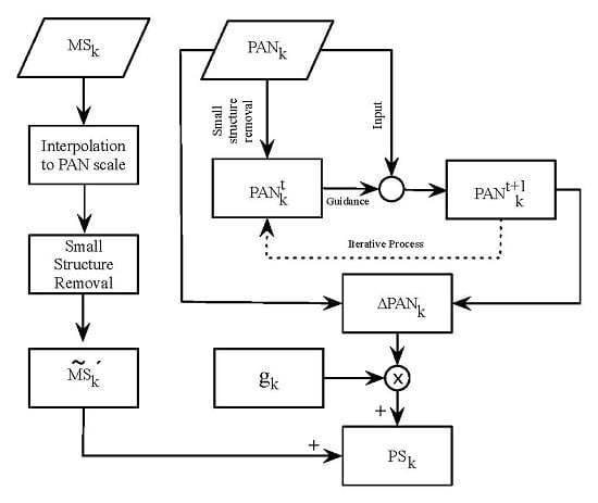
3. Proposed Pansharpening Method Based on the Rolling Guidance Filter

The proposed PS methodology is based on the application of RGF using the MRA approach. It is called the pansharpening rolling guidance filter method (PSRGF); and has four main steps: (i) pre-processing of the images; (ii) small structures are removed from the MS image (low frequency); (iii) edge recovery from the PAN image (high frequency); and (iv) low and high frequency data integration to create a high-resolution multispectral image (pansharpened image). The workflow of the methodology proposed in this work is illustrated in Figure 2.

(i)

Pre-processing of the images: The MS and PAN (source images) were perfectly co-registered and the MS image resized to the PAN image size. In particular, in this work, the $Lanczos3$ algorithm [36] was used, obtaining a $\widetilde{MS}$, that corresponds to the MS image interpolated at the PAN scale. Moreover, a histogram-matched PAN image was produced using Equation (12):

$$PA{N}_k=\frac{{\sigma }_{M{S}_k}}{{\sigma }_{PAN}}(PAN-{\mu }_{PAN})+{\mu }_{M{S}_k}$$

(12)

where μ and σ denote the mean and standard deviation of an image, respectively.

(ii)

Small structure removal: To completely remove structures with a scale of less than ${\sigma }_s$ from the k-th band of the MS image, a weighted average Gaussian filter approach, formalized in Equation (13), was used.

$${\widetilde{MS}}_k^{\prime }\left(p\right)=\frac{1}{K_p^{{\widetilde{MS}}_k}}\sum _{q\in N\left(p\right)}{e}^{-\frac{{\parallel p-q\parallel }^2}{2{\sigma }_s^2}}{\widetilde{MS}}_k\left(q\right)$$

(13)

where ${\widetilde{MS}}_k^{\prime }\left(p\right)$ is the low frequency content for the k-th band of the MS image and corresponds to the first iteration of the bilateral filter ($t=1$), $N\left(p\right)$ is the set of neighboring pixels of p and $K_p^{{\widetilde{MS}}_k}$ is a normalization of ${\widetilde{MS}}_k^{\prime }\left(p\right)$ and defined in Equation (14):

$$K_p^{{\widetilde{MS}}_k}=\sum _{q\in N\left(p\right)}{e}^{-\frac{{\parallel p-q\parallel }^2}{2{\sigma }_s^2}}$$

(14)

(iii)

PAN edge recovery: Equation (15) was applied to recover the edges of the $PA{N}_k$ image, using the result of the RGF process at the t-th iteration:

$$PA{N}_k^{t+1}\left(p\right)=\frac{1}{K_p^{PA{N}_k}}\sum _{q\in N\left(p\right)}(PA{N}_k^{{\sigma }_s}(\parallel p-q\parallel )-PA{N}_k^{{\sigma }_r}(\parallel PA{N}_k^t\left(p\right)-PA{N}_k^t\left(q\right)\parallel \left)\right)PA{N}_k\left(q\right)$$

(15)

To obtain just the high frequency (edges) from the $PA{N}_k$ image, which will be injected into the MS image, the difference between the $PA{N}_k$ and $PA{N}_k^{t+1}$ image was calculated, using the Equation (16):

$$\Delta PA{N}_k\left(p\right)=PA{N}_k\left(p\right)-PA{N}_k^{t+1}\left(p\right)$$

(16)

(iv)

Pansharpening image: The PS image was obtained using the MRA approach, formalized in Equation (17):

$$P{S}_k\left(p\right)={\widetilde{MS}}_k^{\prime }\left(p\right)+g_k\left(p\right)\times \Delta PA{N}_k\left(p\right)$$

(17)

To provide an objective and consistent evaluation of all algorithms involved in this work, a set of seven different spatial, spectral and overall quality indices was used. The name, equation, ideal value and the authors of each of the indices are shown in

Table 2. Quality indices for the evaluation pansharpened images. k denotes the k-th band, ${\sigma }_{x,y}$ the co-variance, ${\sigma }_x^2$ the variance, ${\mu }_x$ the mean value, z and v are hypercomplex representations of the image.

Index	Equation	Ideal Value	Reference
${\mathrm{Q}}_k$	$\frac{{\sigma }_{M{S}_k,P{S}_k}}{{\sigma }_{M{S}_k}{\sigma }_{P{S}_k}}\times \frac{2\mu M{S}_k\times \mu P{S}_k}{{\left(\mu M{S}_k\right)}^2+{\left(\mu P{S}_k\right)}^2}\times \frac{2{\sigma }_{M{S}_k}{\sigma }_{P{S}_k}}{{\sigma }_{M{S}_k}^2+{\sigma }_{P{S}_k}^2}$	1	[37]
${\mathrm{SAM}}_k$	$co{s}^{-1}\frac{\langle M{S}_k,P{S}_k\rangle }{\parallel M{S}_k\parallel \parallel P{S}_k\parallel }$	$0^{°}$	[38]
ERGAS	$100\frac{h}{l}\sqrt{\frac{1}{N}{\sum }_{i=1}^{\#Bands}(\frac{RMSE{(M{S}_i,P{S}_i)}^2}{{\left(M{S}_i\right)}^2})}$	0	[39]
SERGAS	$100\frac{h}{l}\sqrt{\frac{1}{N}{\sum }_{i=1}^{\#Bands}}(\frac{RMSE{(PA{N}_i,P{S}_i)}^2}{{\left(PA{N}_i\right)}^2})$	0	[11]
$CC$	$\frac{1}{\#Bands}{\sum }_{i=1}^{\#Bands}cor{r}_i(M{S}_i,P{S}_i)$	1	[39]
Q$2^n$	$\frac{{\sigma }_{z,v}}{{\sigma }_z{\sigma }_v}\times (\frac{2\overline{z}\times \overline{v}}{{\overline{z}}^2+{\overline{v}}^2})\times \frac{2{\sigma }_z{\sigma }_v}{{\sigma }_z^2+{\sigma }_v^2}$	1	[40]
${\mathrm{SSIM}}_k$	$\frac{(2{\mu }_{M{S}_k}{\mu }_{PA{N}_k}+C_1)(2{\sigma }_{M{A}_{k}P{S}_k}+C_2)}{({\mu }_{M{S}_k}^2+{\mu }_{PA{N}_k}^2+C_1)({\sigma }_{M{S}_k}^2+{\sigma }_{PA{N}_k}^2+C_2)}$	1	[41]

. Considering the diverse nature of the indices used to determine the quality of the pansharpened images, a single quality ranking has been defined based on the consensus of the values of the seven indices in order to facilitate its later analyses. In this regard, the Borda count (BC) [29] method was selected for its simplicity and popularity. The BC count is a single-winner choice method in which voters rank options or candidates in order of preference and is often described as a consensus-based ranking system rather than a majority one. For a comprehensive description of BC, please refer to Zhang et al. [30].

4. Results and Discussion

Three versions of the PS method based on the RGF were defined from Equation (17). The difference between them lies in the definition of the gain $g_k$. The first one integrates 100% of the edge information ($FG$) obtained from the application of the RGF process to PAN. The second and third methods integrate weighted information, using the luminance proportional (LP) and the average value of the entropy (E) of the MS and PAN, respectively, as $g_k$. The names and gain injection equations of the proposed methods are shown in

Table 3. Injection gain ($g_k$) through an element-by-element multiplication of the spatial details from the PAN to be integrated with the MS image to obtain the PS image and the three names of the corresponding PS algorithms.

Injection Gain (${\mathit{g}}_{\mathit{k}}$)	${\mathit{g}}_{\mathit{k}}$ Equation	PS Method
Full Gain (FG)	1	${\mathrm{PSRGF}}_{FG}$
Luminance Proportional (LP)	$\frac{\widetilde{M{S}_k}}{\frac{1}{\#Bands}{\sum }_{i=1}^{\#Bands}\widetilde{M{S}_i}}$	${\mathrm{PSRGF}}_{LP}$
Entropy (E)	$\frac{S\left(M{S}_k\right)+S\left(PA{N}_k\right)}{2}$	${\mathrm{PSRGF}}_E$

. The proposed methods were compared with five widely-used algorithms in the literature: WATFRAC [5], BT [16], IHS [13], GS [15] and MTF–GLP [28].

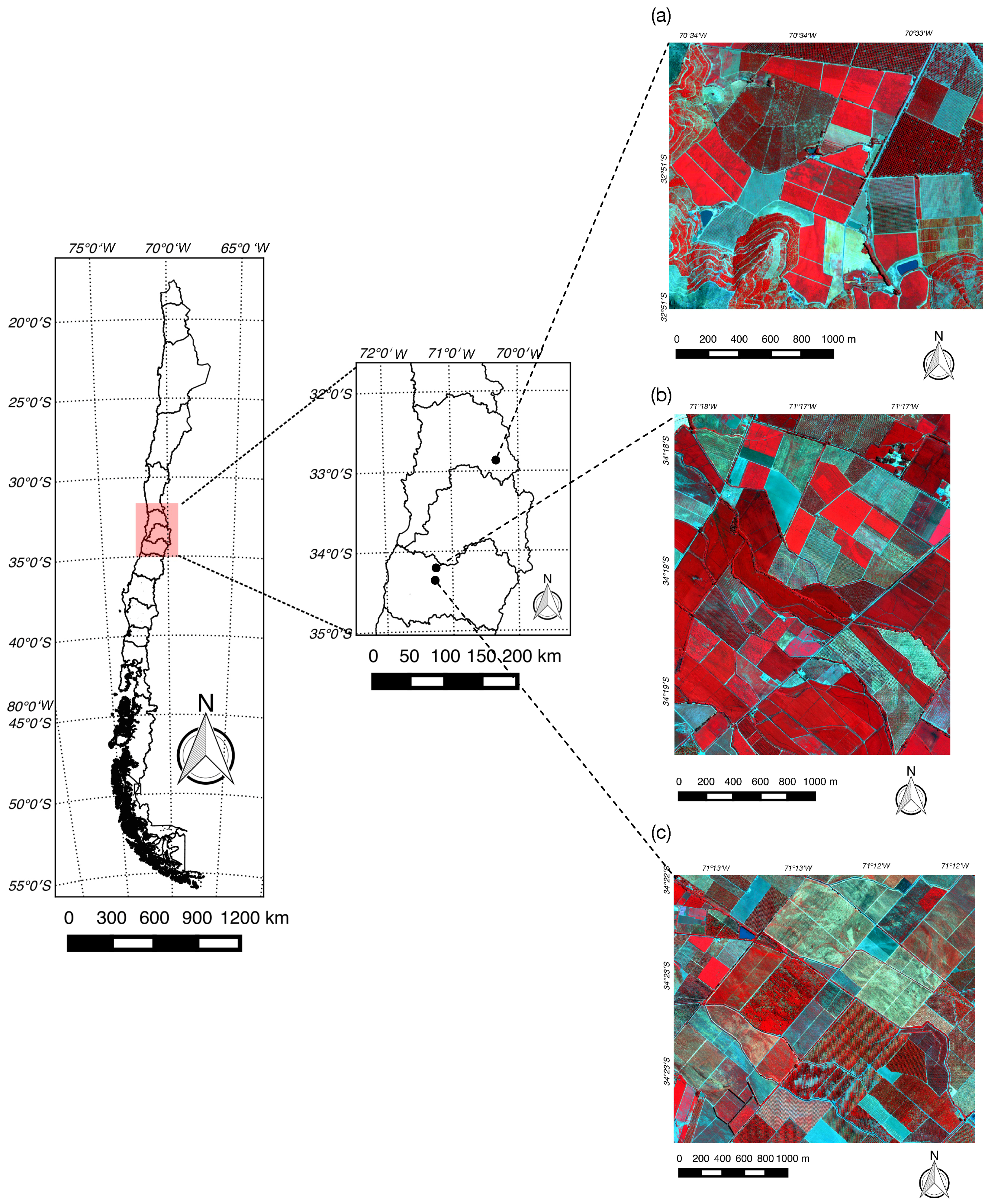
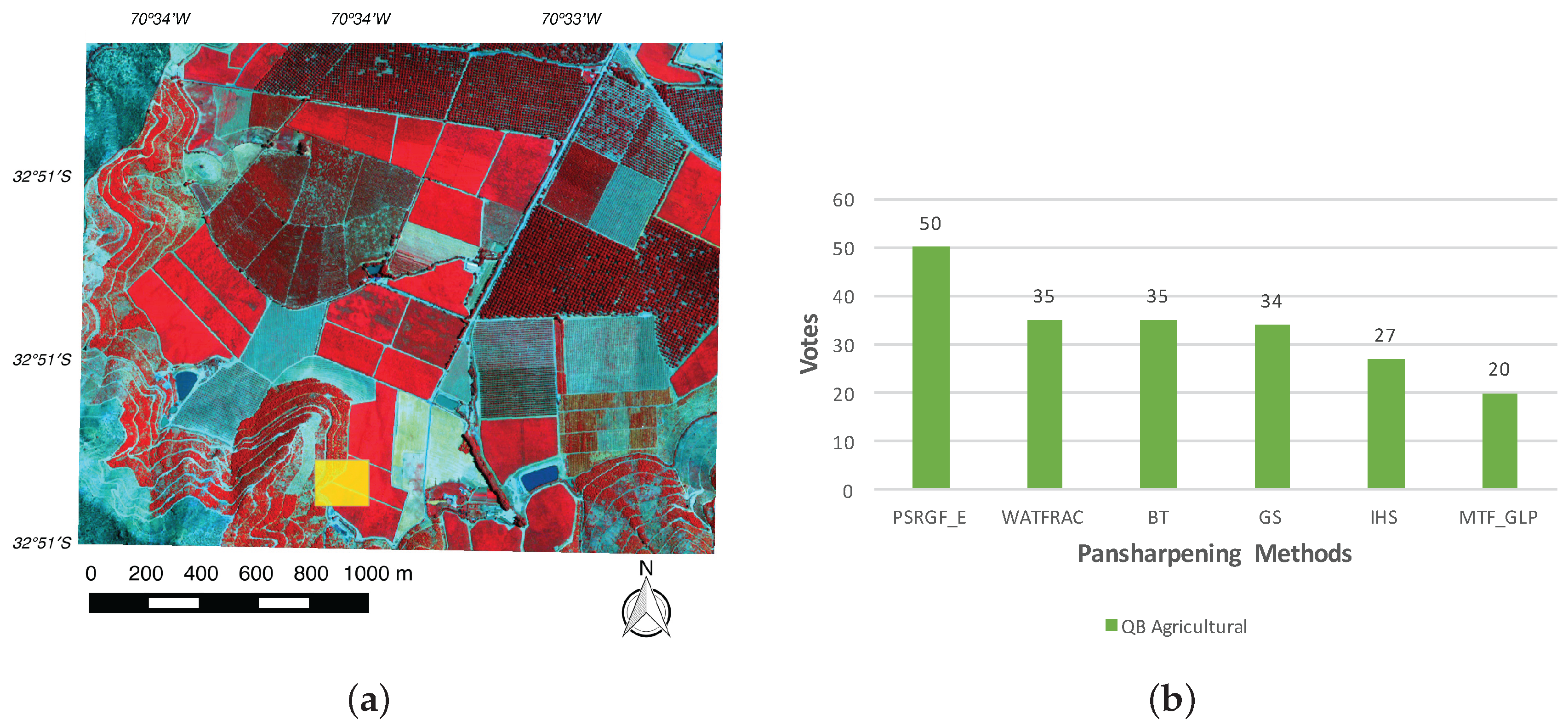
4.1. Testing Dataset

For the application and evaluation of the proposed algorithms and their later comparison with the most used methods, three images were used in which there are predominantly highly fragmented agricultural-type covers. The first image corresponds to a scene captured by the QuickBird–2 (QB) sensor on 16 January 2012 over the Los Andes city, in the region of Valparaiso, Chile (${32}^{°}{51}^{\prime }$S:${70}^{°}{34}^{\prime }$W), identified in this work as QB Agricultural. The other two images correspond to a scene captured by the Worldview–2 (WV) sensor on 10 January 2012 over the city of Peumo, in the region of O’Higgins, Chile; the first of them identified in this work as WV Agricultural 1 (${34}^{°}{19}^{\prime }$S:${71}^{°}{17}^{\prime }$W) and the second one as WV Agricultural 2 (${34}^{°}{23}^{\prime }$S:${71}^{°}{13}^{\prime }$W). The three images use the EPSG:32719–WGS 84/UTM Zone 19S coordinate reference system. In Figure 3, it is possible to observe their geographical location. In Figure 3a–c, a predominance of highly-fragmented agricultural-type covers can be seen, with different types of crops and orchards.

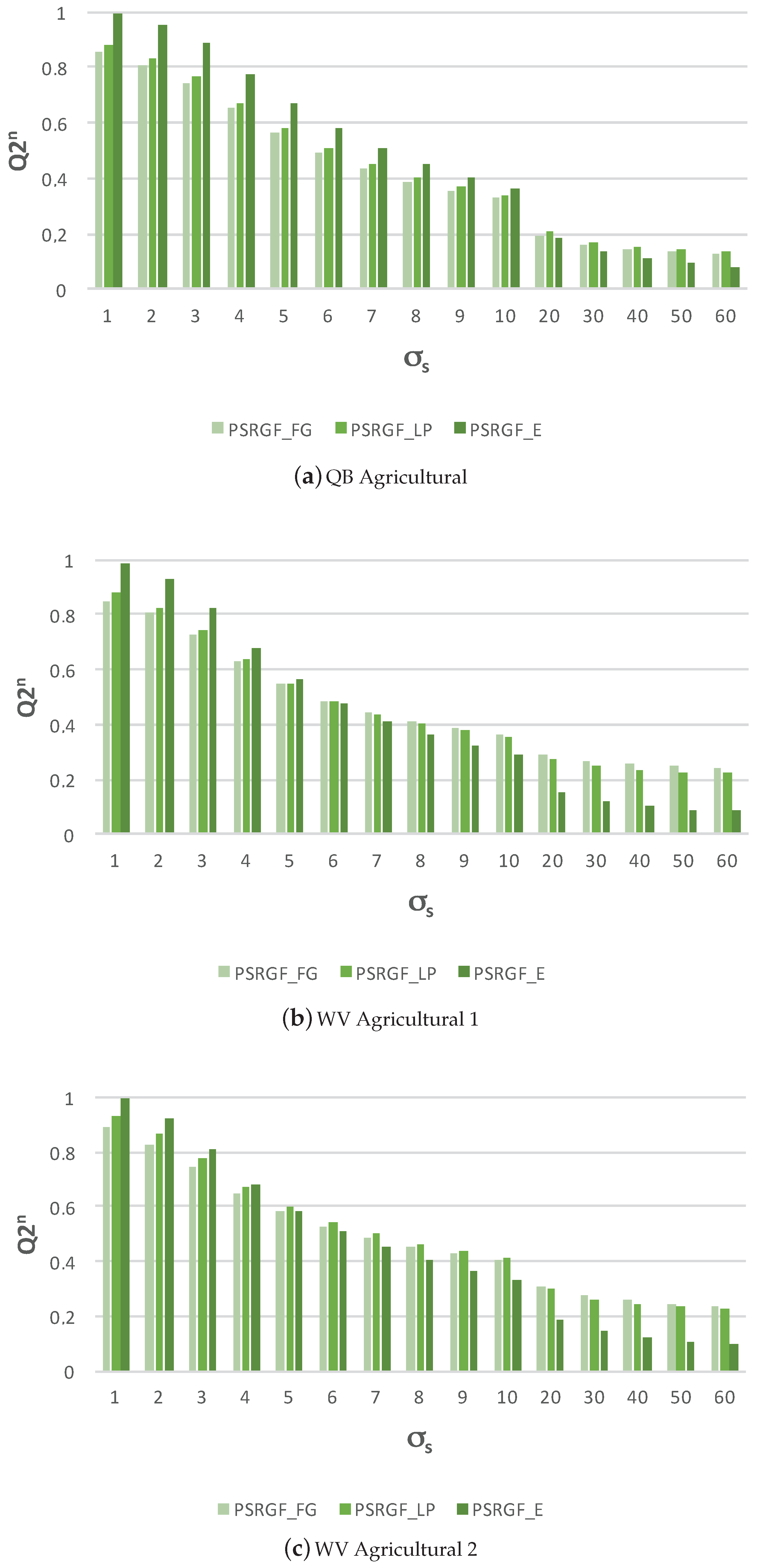
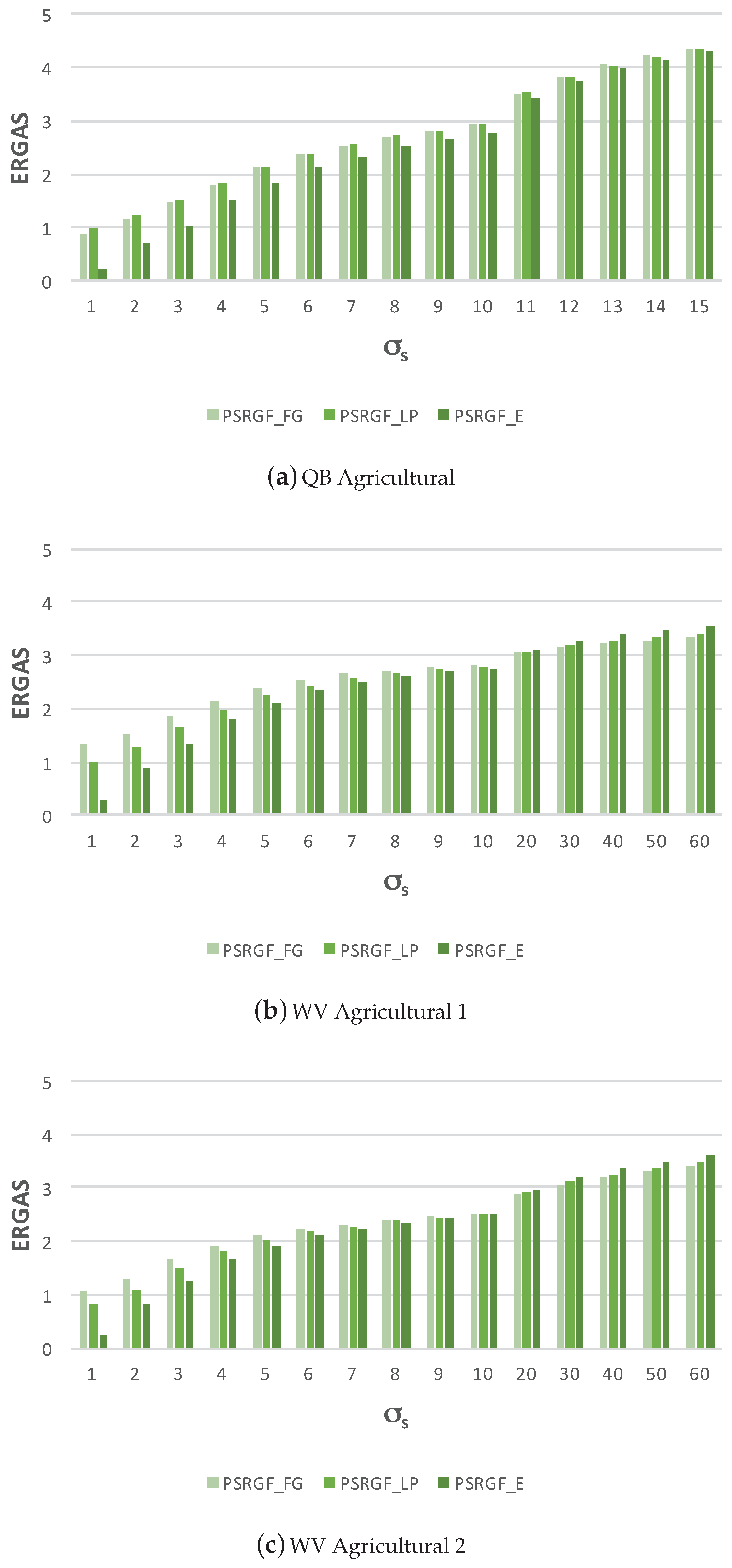
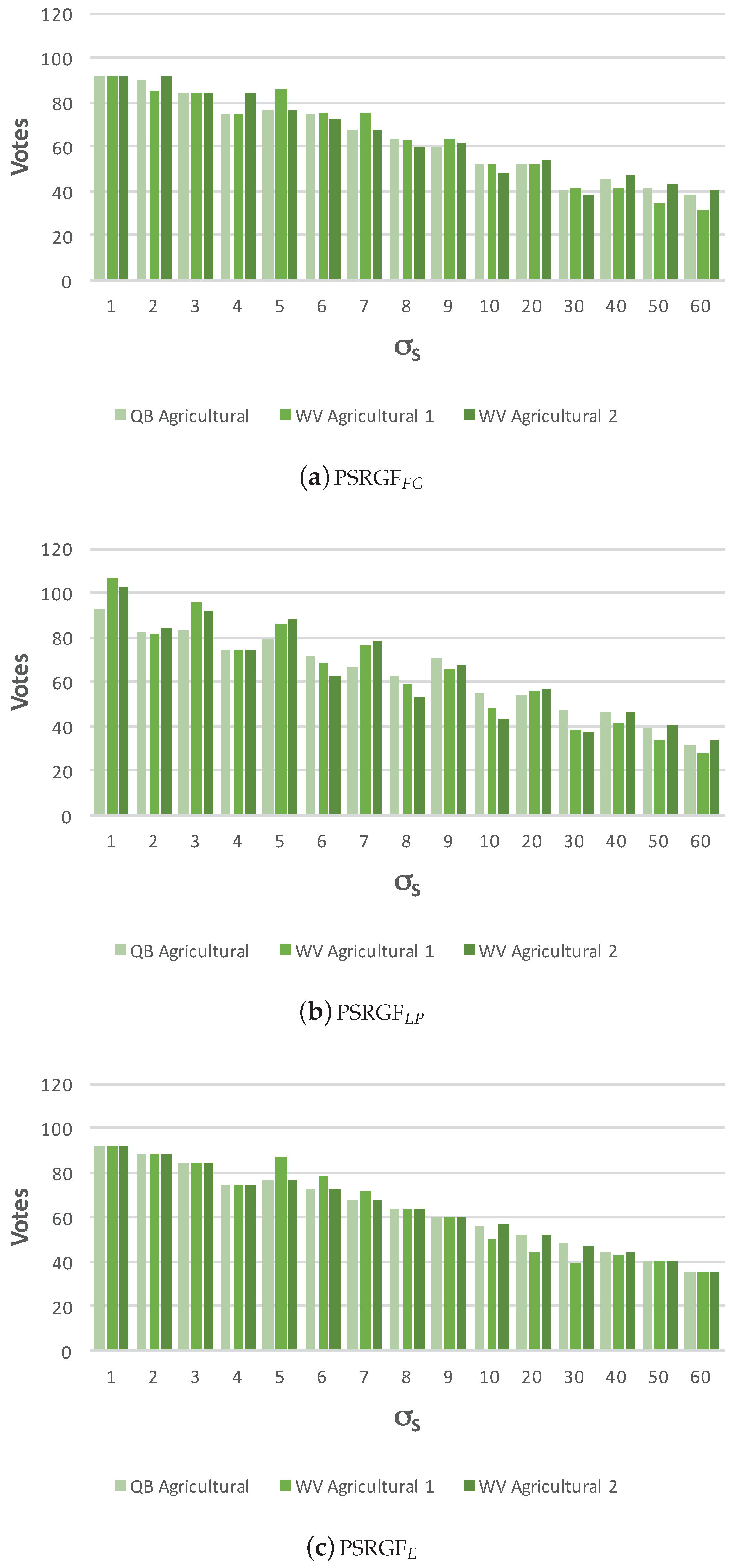
4.2. Quality Assessment

The three test images were pansharpened using the methodology proposed in Section 3 and considering the $g_k$ defined in Table 3 (${\mathrm{PSRGF}}_{FG}$, ${\mathrm{PSRGF}}_{LP}$ and ${\mathrm{PSRGF}}_E$).

There are three main parameters in the methodology proposed (PSRGF), those determined by the RGF process, which are: the scale of the structures to be eliminated (${\sigma }_s$), the level of influence of the neighboring pixels in respect to the pixel analyzed (${\sigma }_r$) and the number of iterations (t). Of the tests carried out in this work and the three parameters, ${\sigma }_s$ is the one with the greatest influence on the quality of the pansharpened images.

With the objective of analyzing and visualizing the influence of this parameter on the quality of the pansharpened images, experiments were carried out on a wide range of ${\sigma }_s$ values (${\sigma }_s=[1,2,3,4,5,6,7,8,9,10,20,30,40,50,60]$), obtaining a total of 45 pansharpened images for each of the images tested (QB Agricultural, WV Agricultural 1, WV Agricultural 2). The value of ${\sigma }_r$ was determined using Equation (18) [26]:

$${\sigma }_r=\frac{max!\left(PAN\right)-min!\left(PAN\right)}{max!\left(PAN\right)}$$

(18)

where $max!$ and $min!$ represent the maximum and minimum value of an image. Furthermore, in this work, a number of iterations $t=4$ were used.

Considering the large number of results obtained from the three test images, the three PS methods proposed, the fifteen values of ${\sigma }_s$ evaluated and the seven quality indices used, it is difficult to show the totality of the results in this work. Therefore, it was decided to show only the behavior of two widely-used indices (Q$2^n$ and ERGAS), which clearly show how the quality of pansharpened images vary with the variation of ${\sigma }_s$.

In Figure 4 and Figure 5, it is possible to see the behavior of the Q$2^n$ and ERGAS indices, in view of the ${\sigma }_s$ variations, for the three test images. For both indices, a loss is observed in the quality of the pansharpened images as the value of ${\sigma }_s$ increases. This result agrees with that reported in Zhang et al. [26], given that the greatest values of ${\sigma }_s$ eliminate a large number of structures, both from the MS and PAN images, thus deteriorating the spatial quality of the pansharpened images.

On evaluating the behavior of the $Q{2}^n$ index, the best result is obtained for the ${\mathrm{PSRGF}}_E$ method when the values of ${\sigma }_s\le 10$ are considered for the QB Agricultural image, ${\sigma }_s\le 6$ for the WV Agricultural 1 image and ${\sigma }_s\le 4$ for the WV Agricultural 2 image. For the case of the ERGAS index, the best behavior was also obtained for the ${\mathrm{PSRGF}}_E$ image; however, the values of ${\sigma }_s$ differed from the previous cases; thus, for the QB Agricultural image, all of the values of ${\sigma }_s$ used delivered the best evaluation of ERGAS by the ${\mathrm{PSRGF}}_E$ method. Finally, both for the WV Agricultural 1 and the WV Agricultural 2 images, the best evaluation of ERGAS for the ${\mathrm{PSRGF}}_E$ method were obtained, considering values of ${\sigma }_s\le 10$.

With the objective of determining the value of ${\sigma }_s$ with which the best pansharpened images for each one of the three methods proposed are obtained, an overall and objective evaluation was carried out on the values obtained for the seven quality indices. For this, a consensus voting process was used, using the BC methodology. In Figure 6a–c, it is possible to see that for the three proposed methods, the value of ${\sigma }_s=1$ is the one that receives the greatest vote, and therefore, it is the one that provides pansharpened images of the greatest quality.

A comparative evaluation was carried out on the quality of the pansharpened images obtained using the proposed methods, as well as the PS methods selected in this study (WATFRAC, BT, GS, IHS, MTF–GLP, ${\mathrm{PSRGF}}_{FG}({\sigma }_s=1)$, ${\mathrm{PSRGF}}_{LP}({\sigma }_s=1)$ and ${\mathrm{PSRGF}}_E({\sigma }_s=1)$). Just as in for the evaluation of the best value of ${\sigma }_s$, a consensus voting process was carried out, using the BC methodology in which the seven quality indices used for the evaluation were considered. The result of this evaluation is summarized in Figure 7, in which it can be seen that for the three test images used, the greatest votes were obtained for the ${\mathrm{PSRGF}}_{FG}$, ${\mathrm{PSRGF}}_{LP}$ and ${\mathrm{PSRGF}}_E$ methods, having used a value of ${\sigma }_s=1$ in all three cases. Of the three methods, ${\mathrm{PSRGF}}_E$ was that which obtained the highest vote for the three test images.

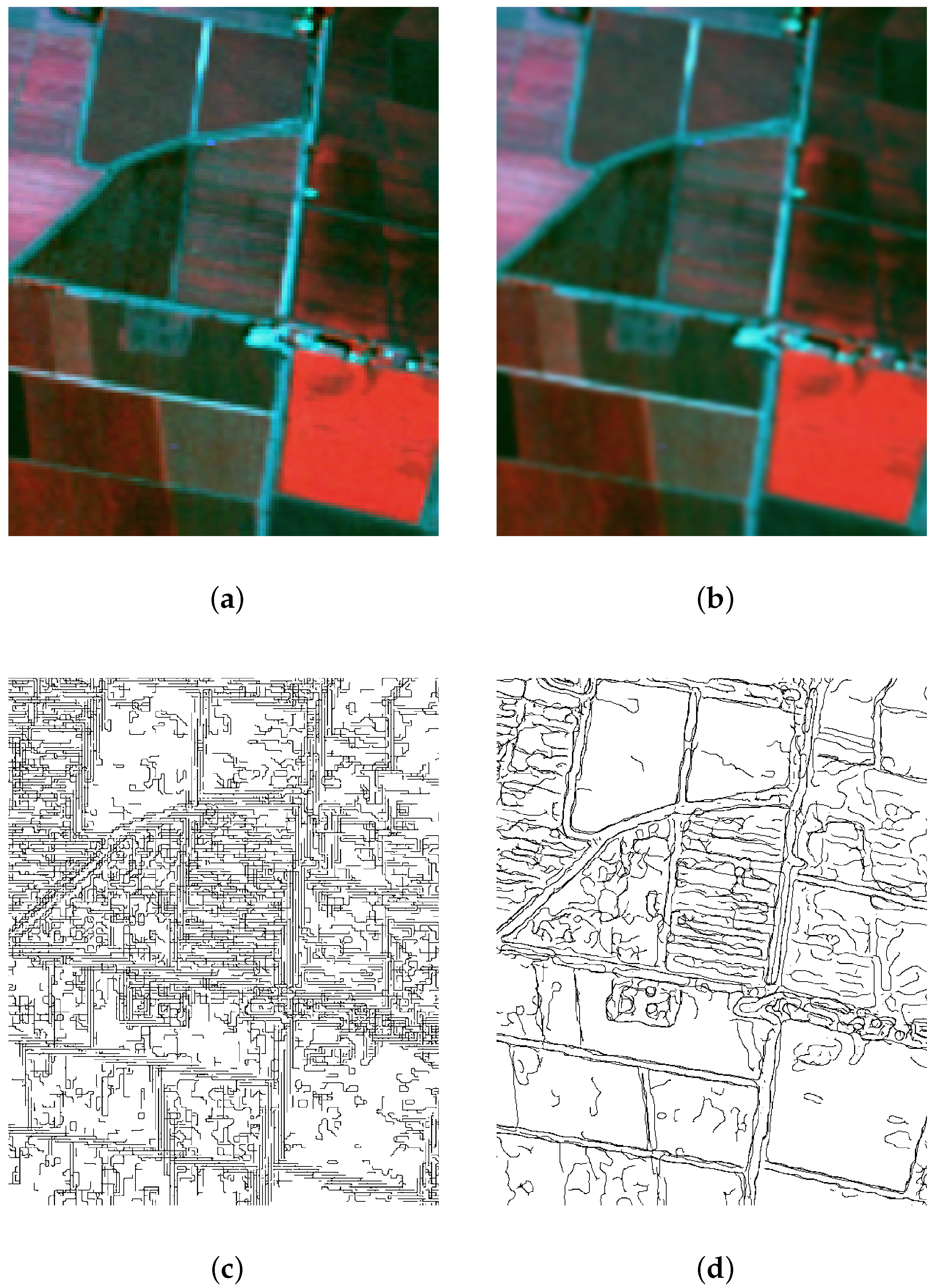
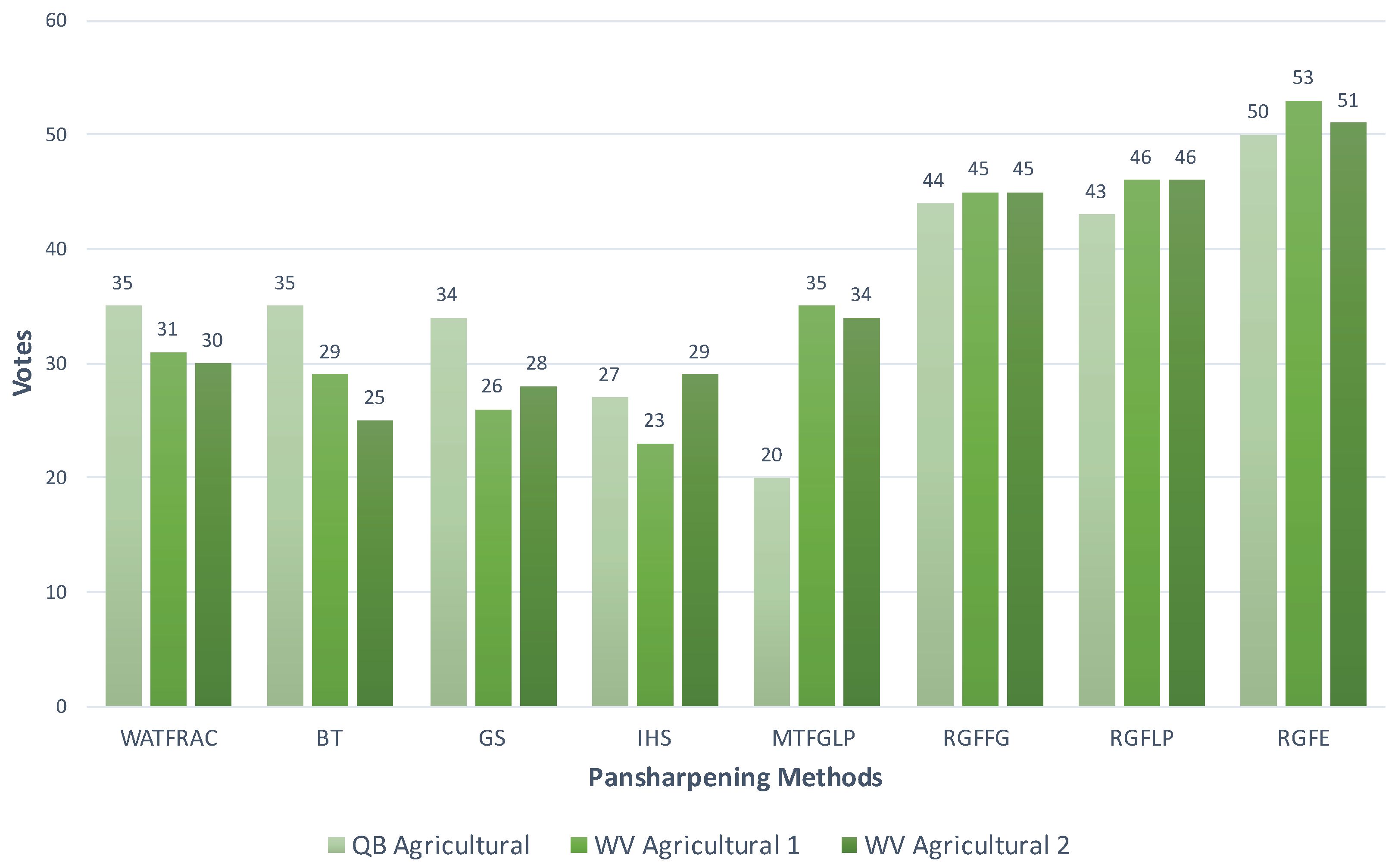
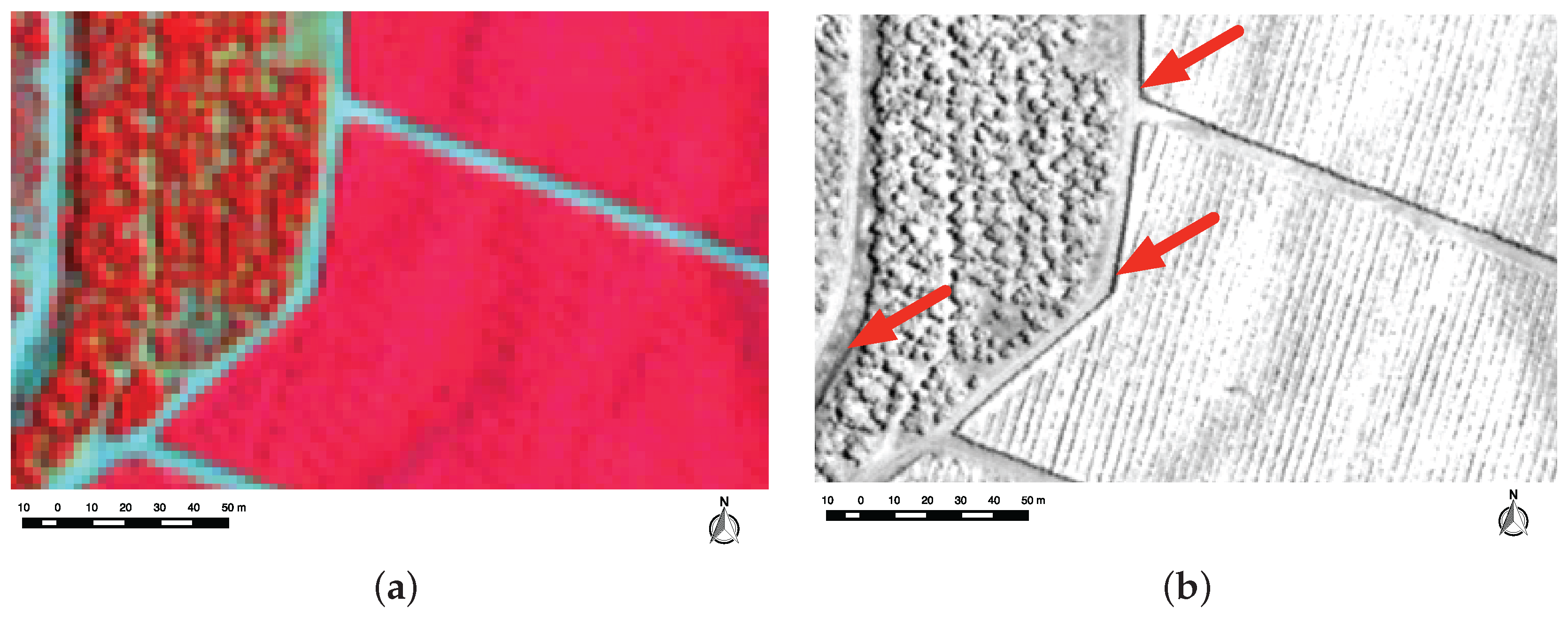
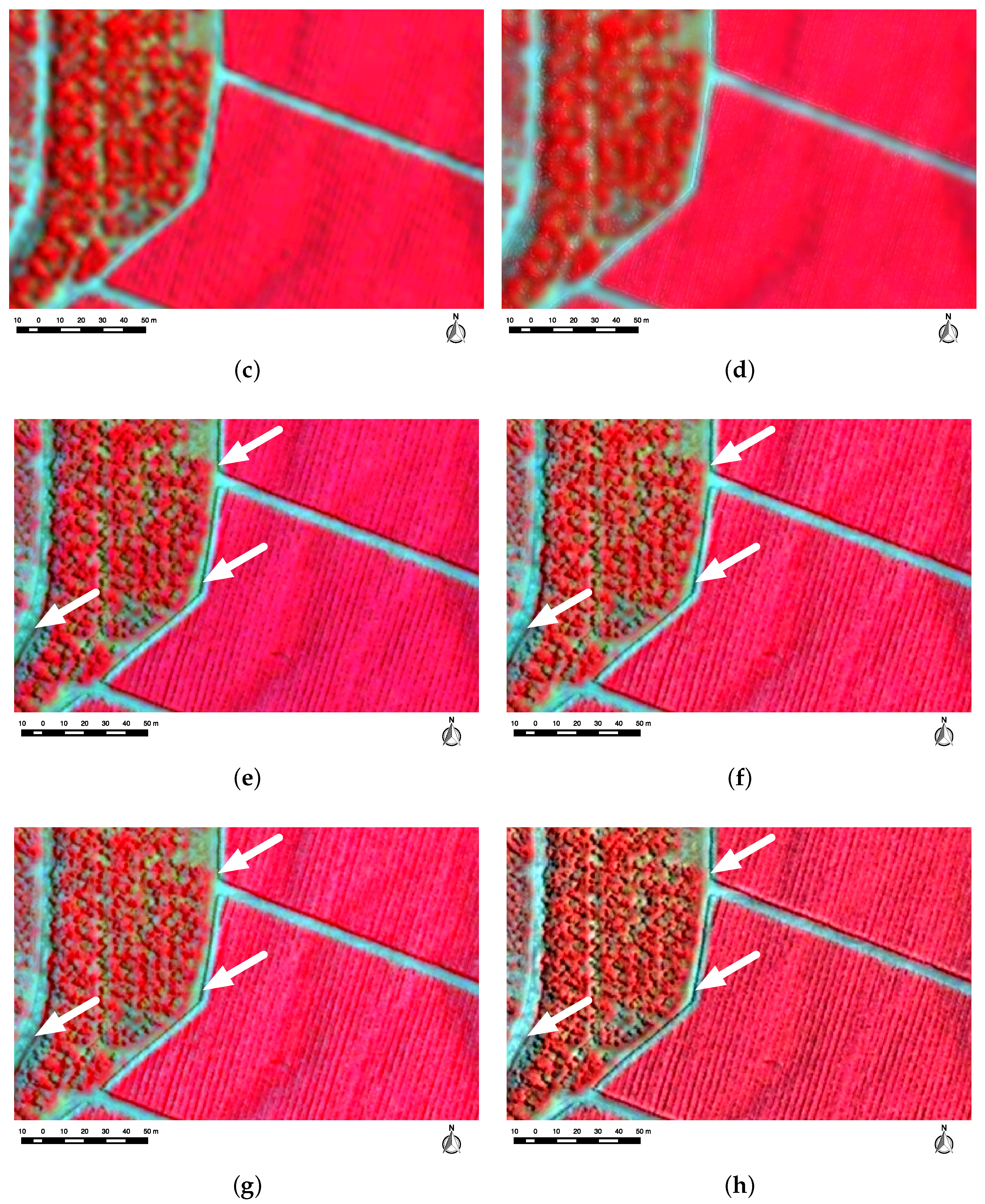
4.3. Visual Assessment of the Pansharpened Images

As well as carrying out a quantitative evaluation of the pansharpened images, a visual analysis of the QB Agricultural test image (Figure 8a) was carried out. With the objective of facilitating the visual analyses, the area of analysis was reduced to a particular area represented in Figure 8a (yellow box). Furthermore, BC was used with the objective of ordering the pansharpened images through the different methods, in agreement with their quality. In this case, only the ${\mathrm{PSRGF}}_E({\sigma }_s=1)$ method was included, as it is the one that provides the best quality from among the proposed methods. The order according to the consensus vote obtained is shown in Figure 8b. Considering this order, the area of analysis for the QB Agricultural MS and PAN is shown in Figure 9a, b, respectively. The area of analysis for the pansharpened images using the ${\mathrm{PSRGF}}_E({\sigma }_s=1)$, WATFRAC, BT, GS, IHS and MTF–GLP methods is shown in Figure 9c–h, respectively.

The BT, GS, IHS y MTF–GLP methods (Figure 9e–h) inject artifacts both within the agricultural plot and at the edges. The latter is evident on the vertical edges of the plots, where as a result of the shadows brought about by the position of the sun at the time of taking the image (E–W), false edges on the road appear. These false edges come from the shadow registered in the PAN image, which are injected, without adapting the scale into the pansharpened image. For the case of the image obtained by the WATFRAC method, which was proposed as a method to reduce the artifacts in the pansharpened images [5], these false edges do not appear; however, there is a very drastic reduction in the variability of the pansharpened image, losing spatial resolution.

Finally, the result obtained with the ${\mathrm{PSRGF}}_E({\sigma }_s=1)$ method (Figure 9c) improves the definition of the boundaries of the agricultural plots, without injecting a high variability within the plot and avoiding the injection of false edges like that revealed in Figure 9e–h. The capacity of the proposed method for eliminating artifacts lies in the filtering (RGF), which allows a complete control of the smoothing procedure (scale-aware) by means of the ${\sigma }_s$ parameter, which can preserve large-scale structures from the MS image and the small structure removal and edge recovery from the PAN image.

4.4. Discussion

The results obtained demonstrate the good performance of the PSRGF method over the fragmented agricultural landscape. The BC results (Figure 6) suggest that regardless of how fragmented the analyzed landscape is, the performance of PSRGF is similar (i.e., the same number of votes). This is in accordance with the results reported by Zhang et al. [26] on the capability of the RGF to remove different levels of detail in natural images with the complete control of detail smoothing. The main advantage of the PSRGF is based on this capability, allowing artifact-free high spatial resolution pansharpened images to be produced, improving the MS edges in images with a fragmented agricultural landscape.

The main drawback of the proposed PS methodology based on RGF is the lack of an objective criterion for selecting a suitable value of ${\sigma }_s$ depending on the user requirements. Specific studies are necessary to resolve this issue. In particular, the fitness function definition that meets the eligibility criterion set out by the users is the most challenging task.

5. Conclusions

This work has demonstrated the potential of the RGF filtering method to develop a PS strategy for specific applications in highly-fragmented agricultural landscapes (PSRGF); in particular, three PS methods were proposed (${\mathrm{PSRGF}}_{FG}$, ${\mathrm{PSRGF}}_{LP}$ and ${\mathrm{PSRGF}}_E$). These methods were compared with five PS methods, widely used in the literature (WATFRAC, BT, $GS$, IHS, MTF–GLP), by means of the evaluation of seven quality indices, which were summarized through a weighted voting strategy (BC). The best result was obtained using the proposed ${\mathrm{PSRGF}}_E$ (${\sigma }_s=1$) algorithm.

Furthermore, a visual evaluation was carried out on one of the three images tested. The main result of this evaluation was that the methods based on PSRGF allow the complete control of the spatial information of the source images that will be fused, thus avoiding the injection of artifacts into the pansharpened images.

The characteristics of the PSRGF method allow pansharpened images to be generated with a sharp definition of the boundaries of the agricultural plots without injecting artifacts or false details, enabling accurate agricultural analysis tasks to be performed.

References

1. Löw, F.; Duveiller, G. Defining the spatial resolution requirements for crop identification using optical remote sensing. Remote Sens. 2014, 6, 9034–9063. [Google Scholar] [CrossRef]
2. Imukova, K.; Ingwersen, J.; Streck, T. Determining the spatial and temporal dynamics of the green vegetation fraction of croplands using high-resolution RapidEye satellite images. Agric. For. Meteorol. 2015, 206, 113–123. [Google Scholar] [CrossRef]
3. Lowder, S.K.; Skoet, J.; Raney, T. The number, size, and distribution of farms, smallholder farms, and family farms worldwide. World Dev. 2016, 87, 16–29. [Google Scholar] [CrossRef]
4. Garcia-Pedrero, A.; Gonzalo-Martin, C.; Fonseca-Luengo, D.; Lillo-Saavedra, M. A GEOBIA methodology for fragmented agricultural landscapes. Remote Sens. 2015, 7, 767–787. [Google Scholar] [CrossRef]
5. Lillo-Saavedra, M.; Gonzalo, C.; Lagos, O. Toward reduction of artifacts in fused images. Int. J. Appl. Earth Obs. Geoinf. 2011, 13, 368–375. [Google Scholar] [CrossRef] [Green Version]
6. Pohl, C.; van Genderen, J. Remote sensing image fusion: An update in the context of Digital Earth. Int. J. Digi. Earth 2014, 7, 158–172. [Google Scholar] [CrossRef]
7. Vaibhav, R.; Pandit, R.; Bhiwani, J. Image fusion in remote sensing applications: A review. Int. J. Comput. Appl. 2015, 120, 22–32. [Google Scholar]
8. Vivone, G.; Alparone, L.; Chanussot, J.; Mura, M.D.; Garzelli, A.; Licciardi, G.A.; Restaino, R.; Wald, L. A critical comparison among pansharpening algorithms. IEEE Trans. Geosci. Remote Sens. 2015, 53, 2565–2586. [Google Scholar] [CrossRef]
9. Aiazzi, B.; Alparone, L.; Baronti, S.; Selva, M. Twenty-five years of pansharpening. In Signal and Image Processing for Remote Sensing, 2nd ed.; CRC Press: Boca Raton, FL, USA, 2012; pp. 533–548. [Google Scholar]
10. Li, S.; Yang, B.; Hu, J. Performance comparison of different multi-resolution transforms for image fusion. Inf. Fusion 2011, 12, 74–84. [Google Scholar] [CrossRef]
11. Lillo-Saavedra, M.; Gonzalo, C. Spectral or spatial quality for fused satellite imagery? A trade-off solution using the wavelet à trous algorithm. Int. J. Remote Sens. 2006, 27, 1453–1464. [Google Scholar] [CrossRef]
12. Garzelli, A.; Nencini, F.; Alparone, L.; Aiazzi, B.; Baronti, S. Pan-sharpening of multispectral images: A critical review and comparison. In Proceedings of the 2004 IEEE International Geoscience and Remote Sensing Symposium ( IGARSS ’04), Anchorage, AK, USA, 20–24 September 2004; pp. 81–84.
13. Koutsias, N.; Karteris, M.; Chuvico, E. The use of intensity-hue-saturation transformation of Landsat-5 Thematic Mapper data for burned land mapping. Photogramm. Eng. Remote Sens. 2000, 66, 829–840. [Google Scholar]
14. Chavez, P.S., Jr.; Kwarteng, A.Y. Extracting spectral contrast in Landsat Thematic Mapper image data using selective principal component analysis. Photogramm. Eng. Remote Sens. 1989, 55, 339–348. [Google Scholar]
15. Laben, C.; Brower, B. Process for Enhancing the Spatial Resolution of Multispectral Imagery Using Pan-Sharpening. U.S. Patent 6,011,875, 4 January 2000. [Google Scholar]
16. Gillespie, A.R.; Kahle, A.B.; Walker, R.E. Color enhancement of highly correlated images. II. Channel ratio and “chromaticity” transformation techniques. Remote Sens. Environ. 1987, 22, 343–365. [Google Scholar] [CrossRef]
17. Gonzalo, C.; Lillo-Saavedra, M. A directed search algorithm for setting the spectral–spatial quality trade-off of fused images by the wavelet à trous method. Can. J. Remote Sens. 2008, 34, 367–375. [Google Scholar] [CrossRef]
18. Khan, M.M.; Alparone, L.; Chanussot, J. Pansharpening quality assessment using the modulation transfer functions of instruments. IEEE Trans. Geosci. Remote Sens. 2009, 47, 3880–3891. [Google Scholar] [CrossRef]
19. Massip, P.; Blanc, P.; Wald, L. A method to better account for modulation transfer functions in ARSIS-based pansharpening methods. IEEE Trans. Geosci. Remote Sens. 2012, 50, 800–808. [Google Scholar] [CrossRef] [Green Version]
20. Ghassemian, H. A review of remote sensing image fusion methods. Inf. Fusion 2016, 32, 75–89. [Google Scholar] [CrossRef]
21. Kaplan, N.; Erer, I. Bilateral filtering-based enhanced pansharpening of multispectral satellite images. IEEE Geosci. Remote Sens. Lett. 2014, 11, 1941–1945. [Google Scholar] [CrossRef]
22. Paris, S.; Kornprobst, P.; Tumblin, J.; Durand, F. Bilateral filtering: Theory and applications. Found. Trends Comput. Graph. Vis. 2008, 4, 1–73. [Google Scholar] [CrossRef]
23. Hu, J.; Li, S. The multiscale directional bilateral filter and its application to multisensor image fusion. Inf. Fusion 2012, 13, 196–206. [Google Scholar] [CrossRef]
24. He, K.; Sun, J.; Tang, X. Guided image filtering. IEEE Trans. Pattern Anal. Mach. Intell. 2013, 35, 1397–1409. [Google Scholar] [CrossRef] [PubMed]
25. Liu, J.; Liang, S. Pan-sharpening using a guided filter. Int. J. Remote Sens. 2016, 37, 1777–1800. [Google Scholar] [CrossRef]
26. Zhang, Q.; Shen, X.; Xu, L.; Jia, J. Rolling guidance filter. In Computer Vision–ECCV 2014; Springer: Berlin, Germany, 2014; pp. 815–830. [Google Scholar]
27. Liu, Y.; Li, M.; Mao, L.; Xu, F.; Huang, S. Review of remotely sensed imagery classification patterns based on object-oriented image analysis. Chin. Geogr. Sci. 2006, 16, 282–288. [Google Scholar] [CrossRef]
28. Aiazzi, B.; Alparone, L.; Baronti, S.; Garzelli, A.; Selva, M. MTF-tailored multiscale fusion of high-resolution MS and pan imagery. Photogramm. Eng. Remote Sens. 2006, 72, 591–596. [Google Scholar] [CrossRef]
29. Emerson, P. The original Borda count and partial voting. Soc. Choice Welf. 2013, 40, 353–358. [Google Scholar] [CrossRef]
30. Zhang, Y.; Zhang, W.; Pei, J.; Lin, X.; Lin, Q.; Li, A. Consensus-based ranking of multivalued objects: A generalized borda count approach. IEEE Trans. Knowl. Data Eng. 2014, 26, 83–96. [Google Scholar] [CrossRef]
31. Amro, I.; Mateos, J.; Vega, M.; Molina, R.; Katsaggelos, A.K. A survey of classical methods and new trends in pansharpening of multispectral images. EURASIP J. Adv. Signal Process. 2011, 2011, 1–22. [Google Scholar] [CrossRef]
32. Aiazzi, B.; Baronti, S.; Lotti, F.; Selva, M. A Comparison between global and context-adaptive pansharpening of multispectral images. IEEE Geosci. Remote Sens. Lett. 2009, 6, 302–306. [Google Scholar] [CrossRef]
33. Zhou, X.; Liu, J.; Liu, S.; Cao, L.; Zhou, Q.; Huang, H. A GIHS-based spectral preservation fusion method for remote sensing images using edge restored spectral modulation. ISPRS J. Photogramm. Remote Sens. 2014, 88, 16–27. [Google Scholar] [CrossRef]
34. Otazu, X.; Gonzalez-Audicana, M.; Fors, O.; Nunez, J. Introduction of sensor spectral response into image fusion methods. Application to wavelet-based methods. IEEE Trans. Geosci. Remote Sens. 2005, 43, 2376–2385. [Google Scholar] [CrossRef] [Green Version]
35. Bjørke, J.T. Framework for entropy-based map evaluation. Cartogr. Geogr. Inf. Syst. 1996, 23, 78–95. [Google Scholar] [CrossRef]
36. Burger, W.; Burge, M.J. Principles of Digital Image Processing: Core Algorithms, 1st ed.; Springer: Berlin, Germany, 2009. [Google Scholar]
37. Wang, Z.; Bovik, A.C. A universal image quality index. IEEE Signal Process. Lett. 2002, 9, 81–84. [Google Scholar] [CrossRef]
38. Kruse, F.; Lefkoff, A.; Boardman, J.; Heidebrecht, K.; Shapiro, A.; Barloon, P.; Goetz, A. Interactive visualization and analysis of imaging spectrometer data. Remote Sens. Environ. 1993, 44, 145–163. [Google Scholar] [CrossRef]
39. Wald, L. Quality of high resolution synthesised images: Is there a simple criterion. In Third Conference “Fusion of Earth Data: Merging Point Measurements, Raster Maps and Remotely Sensed Images”; Ranchin, T., Wald, L., Eds.; SEE/URISCA: Sophia Antipolis, France, 2000; pp. 99–103. [Google Scholar]
40. Garzelli, A.; Nencini, F. Hypercomplex quality assessment of multi/hyperspectral images. IEEE Geosci. Remote Sens. Lett. 2009, 6, 662–665. [Google Scholar] [CrossRef]
41. Wang, Z.; Bovik, A.C.; Sheikh, H.R.; Simoncelli, E.P. Image quality assessment: From error visibility to structural similarity. IEEE Trans. Image Process. 2004, 13, 600–612. [Google Scholar] [CrossRef] [PubMed]
Figure 1. Comparison between original and rolling guidance filter (RGF) filtered images and their edges. (a) Original multispectral (MS) image; (b) MS filtered image using RGF ( t = 4 , σ s = 3 and σ r = 0 . 2 ); (c) MS edges obtained from their gray scale version using the Canny filter; and (d) Edges of the filtered MS using RGF, obtained from the gray scale version using the Canny filter.
Remotesensing 08 00870 g001
Figure 2. Workflow of the pansharpening (PS) proposed method based on the rolling guidance filter (PSRGF). M S k and P A N k are the k-th band of the MS and histogram-matched PAN images and P A N t + 1 the last update of the RGF iteration process.
Remotesensing 08 00870 g002
Figure 3. Source images: (a) QuickBird–2 (QB) Agricultural, located at 32 ° 51 S: 70 ° 34 W; (b) Worldview–2 (WV) Agricultural 1, located at 34 ° 19 S: 71 ° 17 W; and (c) WV Agricultural 2, located at 34 ° 23 S: 71 ° 13 W.
Remotesensing 08 00870 g003
Figure 4. Q 2 n index behavior: (a) PSRGF F G ; (b) PSRGF L P and (c) PSRGF E methods for different σ s values.
Remotesensing 08 00870 g004
Figure 5. ERGAS index behavior: (a) PSRGF F G ; (b) PSRGF L P and (c) PSRGF E methods for different σ s values.
Remotesensing 08 00870 g005
Figure 6. Comparison of the quality indexes set of pansharpened images obtained by: (a) PSRGF F G ; (b) PSRGF L P and (c) PSRGF E for different values of σ s , using Borda count (BC).
Remotesensing 08 00870 g006
Figure 7. Comparison of the quality indexes set of pansharpened images obtained by WATFRAC, Brovey transform (BT), Grand–Schmidt (GS), intensity-hue-saturation (IHS), modulation transfer function (MTF–GLP), PSRGF F G ( σ s = 1 ) , PSRGF L P ( σ s = 1 ) and PSRGF E ( σ s = 1 ) , using BC.
Remotesensing 08 00870 g007
Figure 8. (a) QB Agricultural false color composition (NIR-red-green), and the specific analysis site (yellow box); (b) ranking of the methods, using BC, sorted by votes.
Remotesensing 08 00870 g008
Figure 9. Specific analysis site of QB Agricultural. (a) MS image; (b) PAN image; (c) PSRGF E pansharpened image; (d) WATFRAC pansharpened image; (e) BT pansharpened image; (f) GS pansharpened image; (g) IHS pansharpened image; (h) MTF–GLP pansharpened image.
Remotesensing 08 00870 g009aRemotesensing 08 00870 g009b